Short–time rotational diffusion in monodisperse charge–stabilized colloidal suspensions

Abstract

We investigate the combined effects of electrostatic interactions and hydrodynamic interactions (HI) on the short–time rotational self–diffusion coefficient $D_{s}^{r}$ in charge–stabilized suspensions. We calculate $D_{s}^{r}$ as a function of volume fraction $\phi$ for various effective particle charges and various amounts of added electrolyte. The influence of HI is taken into account by a series expansion of the two-body mobility tensors. At sufficiently small $\phi$ this is an excellent approximation due to the strong electrostatic repulsion. For larger $\phi$, we also consider the leading hydrodynamic three–body contribution.

Our calculations show that the influence of the HI on $D_{s}^{r}$ is less pronounced for charged particles than for uncharged ones. Salt–free suspensions are particularly weakly influenced by HI. For these strongly correlated systems we obtain the interesting result $D_{s}^{r}=D_{0}^{r}(1-a_{r}\phi^{2})$ for small $\phi$. Here $D_{0}^{r}$ denotes the Stokesian rotational diffusion coefficient, and $a_{r}$ is a positive parameter which is found to be nearly independent of the particle charge. The quadratic $\phi$–dependence can be well explained in terms of an effective hard sphere model.

Experimental verification of our theoretical results for $D^{r}_{s}$ is possible using depolarized dynamic light scattering from dispersions of optically anisotropic spherical particles.

1 Introduction

Until several years ago, the major interest in the dynamics of colloidal suspensions was focussed on the investigation of translational diffusion. The properties of translational collective and self–diffusion have been studied in great detail both experimentally [1] and theoretically [2, 3, 4]. Information on the translational diffusion is contained in the dynamic structure factor $S(q,t)$, which can be probed for a certain range of wavenumbers $q$ and correlation times $t$ using dynamic light scattering from essentially monodisperse particles [1].

More recently, considerable effort was made to investigate also the rotational diffusion in suspensions of spherically shaped colloidal particles, which possess an intrinsic optical anisotropy due to a partially crystalline structure [5, 6]. To investigate the rotational particle diffusion, one has to resort to depolarized dynamic light scattering (DDLS), which is sensitive on the temporal self–correlations both in the particle positions and orientations. With this technique, the information on the short–time rotational diffusion is obtained from the autocorrelation function $G_{VH}(q,t)$ of the horizontally polarized scattered electric field [7]. From DDLS measurements of the first cumulant of $G_{VH}(q,t)$, one can determine the short–time rotational self–diffusion coefficient $D^{r}_{s}$. The diffusion coefficient $D^{r}_{s}$ depends on the direct potential interactions between the colloidal particles and on the indirect hydrodynamic interactions (HI) mediated by the suspending solvent. The latter interactions account for the fact that the velocity field, generated in the surrounding fluid by the motion of one particle, affects that of the other particles.

By performing DDLS on index–matched suspensions of charged spherical particles made of a fluorinated polymer, Degiorgio et. al. were able to measure in great detail the concentration dependence of the rotational diffusion coefficient [5, 6]. They were mainly interested in suspensions with large salinity, where the particles essentially behave as hard spheres. Their experimental findings for $D^{r}_{s}$ have been compared with recent theoretical calculations by Jones [6, 8], designed for hard sphere suspensions. These calculations include also the approximative evaluation of the coefficient of the quadratic term in the virial expansion of $D^{r}_{s}$ in powers of the volume fraction $\phi$. The agreement between theoretical and experimental results for $D^{r}_{s}$ is found to be satisfactory. Moreover, the small differences observed in the magnitude of the first and second virial coefficients are suggested to be partially due to residual electrostatic interactions, which are left over if the ionic strength of the added electrolyte is not large enough to completely screen the Coulomb repulsion [6].

In fact, the microstructure of a suspension of charged particles depends crucially on the amount of added electrolyte. For charge–stabilized suspensions, the general form of, e.g., the pair distribution function $g(r)$ is qualitatively different from that of hard spheres at the same volume fraction [4]. Due to the large spatial extend of the counterion cloud, the pair potential can have a range much larger than the physical particle diameter $\sigma$. Therefore, appreciable pair correlations become already important at much lower values of the volume fraction $\phi$ as in the case of hard spheres. For this reason, the concentration dependence of $D^{r}_{s}$ can be quite different for uncharged and charged particles, particularly if the amount of added electrolyte becomes low.

In this work, we focus on the combined effects of electrostatic and hydrodynamic interactions on the short–time rotational self–diffusion in charge–stabilized suspensions of spherical particles. Starting from the generalized Smoluchowski equation for the positional and orientational degrees of freedom, we calculate $D^{r}_{s}$ as a function of volume fraction $\phi$ for various effective particle charges and various amounts of added electrolyte. The hydrodynamic interactions are taken into account by a series expansion of the two–body mobility tensors in terms of the reciprocal interparticle distance, $r^{-1}$, by including contributions up to order $r^{-20}$. At sufficiently small $\phi$, this in an excellent approximation due to the strong electrostatic repulsion, which renders configurations of nearly touching particles as extremely unlikely. For larger $\phi$, we consider also the leading hydrodynamic three–body contribution [6], using Kirkwood’s superposition approximation for the triplet correlation function, which is needed as the static input.

We will show that the influence of the HI on $D^{r}_{s}$ is less strong for charge–stabilized particles than for uncharged ones. The influence of HI is particularly weak for suspensions in which all exess ions have been removed. For these strongly correlated systems, we find the remarkable result $D_{s}^{r}=D_{0}^{r}(1-a_{r}\phi^{2})$ for small $\phi$, where $D^{r}_{0}$ is the rotational diffusion coefficient at infinite dilution. The parameter $a_{r}$ is found to be nearly independent of the particle charge for values large enough so that the hard core is completely masked by the electrostatic repulsion. We can explain the quadratic $\phi$–dependence in terms of a simplified calculation based on an effective hard sphere model.

The paper is organized as follows. In Sec. 2, we briefly summarize salient relations of the theory of DDLS from optically anisotropic particles, which are relevant for obtaining the first cumulant of the depolarized field autocorrelation function. For later comparison, we recall in Sec. 3 the theory of short–time rotational diffusion and its main results with regard to suspensions of hard spheres. Sec. 4 gives the details of our calculations of $D^{r}_{s}$ for charge–stabilized suspensions. It contains also a discussion of the range of validity of the various approximations used in this work. We present our results in Sec. 5 and discuss their meaning in terms of simple physical arguments based on an effective hard sphere model. Sec. 6 contains our final conclusion.

2 Depolarized light scattering from anisotropic particles

In this section, we summarize some pertinent relations of the theory of depolarized dynamic light scattering (DDLS) from optically anisotropic particles, which are required for our further discussion. A thorough discussion of general DDLS properties has been given in [5, 6, 7], which allows us to be rather brief in our explanations.

Consider a suspension of identical spherical particles with cylindrically symmetrical optical anisotopy and in a situation in which the incident electric field of the laser beam is linearly polarized perpendicular to the scattering plane. The suspended particles are assumed to be nearly index–matched to the solvent so that the Rayleigh–Gans–Debye approximation is valid even for large volume fractions. The presence of optical anisotropy in the scatterers gives then rise to a non–vanishing horizontally polarized part of the scattered electric field with magnitude

$$E_{VH}(\mbox{\boldmath$q$},t)=f(q)\beta\left(\frac{2\pi}{15}\right)^{\frac{1}{2}}\sum_{l=1}^{N}\left(Y_{2,1}(\mbox{\boldmath$u$}_{l}(t))+Y_{2,-1}(\mbox{\boldmath$u$}_{l}(t))\right)e^{i\mbox{\boldmath\scriptsize$q$}\cdot\mbox{\boldmath\scriptsize$R$}_{l}(t)},$$ (1)

which is not affected by multiply scattered light. Here $N$ is the number of particles in the scattering volume, $q$ is the scattering vector with modulus $q$, and $\mbox{\boldmath$R$}_{l}(t)$ and $\mbox{\boldmath$u$}_{l}(t)$ are the position vector and, respectivly, the unit vector in the direction of the optical axis of the $l$th particle. The $Y_{2,\pm 1}$ are the second–order spherical harmonics of index $\pm 1$, $f(q)$ is the scattering amplitude of a particle, and $\beta=\alpha_{\parallel}-\alpha_{\perp}$, is the internal particle anisotropy, i.e. the difference in the polarizabilities parallel and perpendicular to the optical axis.

In DDLS experiments, one measures the modulus of the temporal correlation function [5, 6]

$$G_{VH}(q,t)=\langle E_{VH}(\mbox{\boldmath$q$},0)E^{*}_{VH}(\mbox{\boldmath$q$},t)\rangle$$ (2)

of the depolarized scattered field, where the bracket indicates for an ergodic system likewise a time or equilibrium ensemble average.

On assuming that the orientation of a particle is decoupled from the particles translation, $|G_{VH}(q,t)|$ can be factorized as [5, 6]

$$|G_{VH}(q,t)|=Nf^{2}(q)\frac{\beta^{2}}{15}F_{s}(q,t)F_{r}(t),$$ (3)

where

$$F_{r}(t)=4\pi\langle Y_{2,1}^{*}(\mbox{\boldmath$u$}_{1}(0))Y_{2,1}(\mbox{\boldmath$u$}_{1}(t))\rangle$$ (4)

is the rotational self–correlation function and

$$F_{s}(q,t)=\langle e^{i\mbox{\boldmath\scriptsize$q$}\cdot[\mbox{\boldmath$\scriptstyle R$}_{1}(0)-\mbox{\boldmath$\scriptstyle R$}_{1}(t)]}\rangle$$ (5)

denotes the translational self–correlation function, also known in the literature as the self–intermediate scattering function. The assumption of translational and rotational decoupling which leads to Eq. (3) can be shown in case of spherically symmetric interacting particles to be rigorously true at short times, i.e. to first order in $t$ in a short–time expansion based on the generalized Smoluchowski equation [3, 6]. At longer times, the assumed decoupling is not strictly valid, but for hard sphere suspensions there is at least experimental evidence that deviations are small for all times [3, 6].

If HI are neglected, $F_{r}(t)$ becomes exponential

$$F_{r}(t)=e^{-6D^{r}_{0}t},$$ (6)

where $D^{r}_{0}=k_{B}T/(8\pi\eta a^{3})$ is the Stokesian rotational diffusion coefficient of a single particle of radius $a$, and $\eta$ is the shear viscosity of the suspending fluid. Eq. (6) arises from the fact that the orientational diffusion of particles with radial symmetric pair interactions are independent from each other if the HI are not considered. In the case of non–interacting spherical particles, $F_{s}(q,t)$ also reduces to an exponential function , i.e. [7]

$$F_{s}(q,t)=e^{-q^{2}D^{t}_{0}t},$$ (7)

where $D^{t}_{0}=k_{B}T/(6\pi\eta a)$ is the translational diffusion coefficient at infinite dilution.

We focus now on the short–time behaviour of interacting colloidal particles. The short–time rotational diffusion coefficient $D^{r}_{s}$ is defined by the short–time behaviour of $F_{r}(t)$ as

$$D^{r}_{s}=-\frac{1}{6}\lim_{t\to 0}\frac{\partial\ln F_{r}(t)}{\partial t}.$$ (8)

This measurable quantity contains the configuration–averaged effects of the HI on the short–time rotational diffusion of a spherical particle. As we will show in the next section, $D^{r}_{s}$ crucially depends an system parameters like the volume fraction $\phi$, the amount of added electrolyte and the effective particle charge. One finds $D^{r}_{s}\rightarrow D^{r}_{0}$ in the limit $\phi\rightarrow 0$.

Notice that the short–time limit $t\rightarrow 0$ in Eq. (8) actually means that $\tau^{r}_{B}\ll t\ll 1/D^{r}_{0}$, with $\tau^{r}_{B}=\Theta/(8\pi\eta a^{3})$ being the relaxation time of the angular momentum of a colloidal sphere with moment of inertia $\Theta$. For uniform spherical particles is $\tau^{r}_{B}\approx\tau^{t}_{B}$, where $\tau^{t}_{B}=m/(6\pi\eta a)$ is the momentum relaxation time of a particle with mass $m$ [3]. It is $\tau^{r}_{B}\approx 10^{-8}s$ for typical suspensions. Most dynamic light scattering experiments are restricted to correlation times $t>10^{-6}s\gg\tau^{r}_{B}$. As a consequence, inertial effects arising from the linear and angular momentum relaxation of the particles are not resolved, so that in DDLS only the relaxation of the particle orientations and positions is probed. This fact allows for a coarse–grained description of Brownian motion on the basis of the generalized Smoluchowski equation, which describes essentialy this relaxation [3, 8]. On this level of description, HI can be considered to act instantaneously.

We further note that $1/D^{r}_{0}=\tau_{I}/3$, where $\tau_{I}=\sigma^{2}/D^{t}_{0}$ is the socalled structural relaxation time, i.e. the time roughly needed for a non–negligible change of the direct interactions due to configurational relaxation. Typically one finds $\tau_{I}\approx 10^{-3}s$ such that the short–time regime $\tau^{r}_{B}\ll t\ll\tau_{I}\approx 1/D^{r}_{0}$ is well seperated from the long–time regime $t\gg\tau_{I}$. For the latter regime, memory effects are important and lead to deviations in $|G_{VH}(q,t)|$ from purely exponential decay.

3 Short–time rotational diffusion

For calculating $D^{r}_{s}$, it is necessary at first to specify the time evolution of the suspended particles. Since we restrict ourselves to correlation times $t\gg\tau^{r}_{B}$, the suspension dynamics is properly described by the generalized Smoluchowski equation. In Smoluchowski dynamics, $F_{r}(t)$ can be expressed as

$$F_{r}(t)=4\pi\langle Y_{2,1}^{*}(\mbox{\boldmath$u$}_{1}(0))e^{\hat{O}^{\dagger}t}Y_{2,1}(\mbox{\boldmath$u$}_{1}(0))\rangle,$$ (9)

where

$$\hat{O}^{\dagger}=\sum_{i,j=1}^{N} \bigg{\{}\left(\nabla_{i}-\frac{1}{k_{B}T}\nabla_{i}\Phi\right)\cdot\left(\mbox{\boldmath$D$}^{tt}_{ij}\cdot\nabla_{j}+\mbox{\boldmath$D$}^{tr}_{ij}\cdot\hat{\mbox{\boldmath$L$}}_{j}\right)+$$ (10)

$$~{}~{}~{}\hat{\mbox{\boldmath$L$}}_{i}\cdot\left(\mbox{\boldmath$D$}^{rt}_{ij}\cdot\nabla_{j}+\mbox{\boldmath$D$}^{rr}_{ij}\cdot\hat{\mbox{\boldmath$L$}}_{j}\right)\bigg{\}},$$

is the adjoint (or backward) Smoluchowski operator [3, 6, 8]. Here $\hat{\mbox{\boldmath$L$}}_{j}=\mbox{\boldmath$u$}_{j}\times\frac{\partial}{\partial\mbox{\boldmath$u$}_{j}}$ is the gradient operator in the compact space of orientations of the $j$th particle, with $\mbox{\boldmath$u$}_{j}$ being the unit vector pointing in the direction of its optical axis. In writing Eq. (10) it has been assumed that the total energy $\Phi=\Phi(\mbox{\boldmath$R$}^{N})$ of the $N$ particles depends only on the center–of–mass positions $\mbox{\boldmath$R$}^{N}=(\mbox{\boldmath$R$}_{1},\ldots\mbox{\boldmath$R$}_{N})$ and not on the particle orientations. We further assume $\Phi$ to be pairwise additive, i.e.

$$\Phi(\mbox{\boldmath$R$}^{N})=\frac{1}{2}\sum_{k,l=1}^{N}\,\!\!\!{}^{\prime}\>u(R_{kl}),$$ (11)

where $u(r)$ is a spherically symmetric pair potential, and $R_{kl}=|\mbox{\boldmath$R$}_{kl}|$ with $\mbox{\boldmath$R$}_{kl}=\mbox{\boldmath$R$}_{k}-\mbox{\boldmath$R$}_{l}$. The prime indicates that the term $k=l$ is excluded from the sum. The diffusivity tensors $\mbox{\boldmath$D$}^{ab}_{ij}$, with $a,b\in\{r,t\}$, embody the HI between the particles by coupling the forces $\mbox{\boldmath$F$}^{N}=(\mbox{\boldmath$F$}_{1},\ldots\mbox{\boldmath$F$}_{N})$ and torques $\mbox{\boldmath$T$}^{N}=(\mbox{\boldmath$T$}_{1},\ldots\mbox{\boldmath$T$}_{N})$ acting on the particles to their translational velocities $\mbox{\boldmath$V$}^{N}=(\mbox{\boldmath$V$}_{1},\ldots\mbox{\boldmath$V$}_{N})$ and angular velocities $\mbox{\boldmath$\omega$}^{N}=(\mbox{\boldmath$\omega$}_{1},\ldots\mbox{\boldmath$\omega$}_{N})$:

$${\mbox{\boldmath$V$}^{N}\choose\mbox{\boldmath$\omega$}^{N}}=\frac{1}{k_{B}T}{\mbox{\boldmath$D$}^{tt}(\mbox{\boldmath$R$}^{N})\mbox{\boldmath$D$}^{tr}(\mbox{\boldmath$R$}^{N})\choose\mbox{\boldmath$D$}^{rt}(\mbox{\boldmath$R$}^{N})\mbox{\boldmath$D$}^{rr}(\mbox{\boldmath$R$}^{N})}{\mbox{\boldmath$F$}^{N}\choose\mbox{\boldmath$T$}^{N}}.$$ (12)

For spherical particles, the diffusivity tensors depend only on the position vectors. The tensors $\mbox{\boldmath$\mu$}^{ab}_{ij}=\mbox{\boldmath$D$}^{ab}_{ij}/(k_{B}T)$ are called mobility tensors.

Using Eqs. (8) and (9), one can express $D^{r}_{s}$ into the form

$$D^{r}_{s}=D^{r}_{0}H^{r}_{s},$$ (13)

and the dimensionless diffusion coefficient $H^{r}_{s}$ is given by

$$H^{r}_{s}=\frac{1}{3D^{r}_{0}}\langle\mbox{Tr}\mbox{\boldmath$D$}^{rr}_{11}(\mbox{\boldmath$R$}^{N})\rangle.$$ (14)

Here $\mbox{Tr}\mbox{\boldmath$D$}^{rr}_{11}$ denotes the sum on the diagonal elements of the tensor $\mbox{\boldmath$D$}^{rr}_{11}$. Due to the many–body nature of the HI, it is not possible to perform an exact evaluation of $H^{r}_{s}$, valid at all particle concentrations. For small volume fractions however, when the mean interparticle distance gets sufficiently large, it becomes possible to obtain a good approximation for $D^{r}_{s}$ by considering only two–body and, to leading order, three–body contributions to the HI.

By using a rooted cluster expansion, Degiorgio et.al. have shown that the normalized short–time rotational diffusion coefficient can be expressed as a series [6]

$$H^{r}_{s}=1+H^{r}_{s1}\phi+H^{r}_{s2}\phi^{2}+H^{r}_{s3}\phi^{3}+\ldots\ .$$ (15)

The coefficient $H^{r}_{s1}$ of the linear term is expressable in term of integrals involving only hydrodynamic two–body contributions and the radial distribution function $g(r)$. Explicitly, $H^{r}_{s1}$ is given by [6, 9]

$$H^{r}_{s1}=\int_{\sigma}^{\infty}dr~{}r^{2}g(r)8\pi\eta\left[\alpha^{rr}_{11}(r)+2\beta^{rr}_{11}(r)\right],$$ (16)

and this expression involves two scalar mobility functions $\alpha^{rr}_{11}(r)$ and $\beta^{rr}_{11}(r)$ depending on the interparticle distance $r$. These functions are calculable by means of a series expansion in even powers of $(a/r)$ [10]. We only quote the leading terms

$$8\pi\eta a^{3}\alpha^{rr}_{11}(r) = -3\left(\frac{a}{r}\right)^{8}+{\mathcal{O}}\left(\left(\frac{a}{r}\right)^{10}\right)$$ (17)

$$8\pi\eta a^{3}\beta^{rr}_{11}(r) = -\frac{15}{4}\left(\frac{a}{r}\right)^{6}-\frac{39}{4}\left(\frac{a}{r}\right)^{8}+{\mathcal{O}}\left(\left(\frac{a}{r}\right)^{10}\right).$$ (18)

Inserting Eqs. (17–18) in Eq. (16) leads to

$$H^{r}_{s1}=\int_{2}^{\infty}dt~{}g(t)\left[-\frac{15}{2}t^{-4}-\frac{45}{2}t^{-6}+{\mathcal{O}}\left(t^{-8}\right)\right]$$ (19)

with $t=r/a$.

The second coefficient $H^{r}_{s2}$ in the expansion of Eq. (15) is for more difficult to evaluate since it involves hydrodynamic three–body contributions. Using the method of reflections, Jones (in Ref. [6]) was able to calculate the leading term in the far–field expansion of the irreducible three–body mobility tensor. Considering only this term, $H^{r}_{s2}$ is approximated by a three–fold integral

$$H^{r}_{s2}=\frac{225}{64}\int^{1}_{0}dt_{12}\int^{1}_{0}dt_{13}\int^{1}_{-1}d\xi_{1}g^{(3)}(t_{12},t_{13},\xi_{1})f(t_{12},t_{13},\xi_{1}),$$ (20)

which involves the static three–particle distribution function $g^{(3)}$ in dependence of $t_{12}=2a/R_{12}$, $t_{13}=2a/R_{13}$, and $\xi=\mbox{\boldmath$R$}_{12}\cdot\mbox{\boldmath$R$}_{13}/(R_{12}R_{13})$. The somewhat lengthy expression for the function $f(t_{12},t_{13},\xi_{1})$ is given in Eqs. (36–37) of Ref. [6] and will not be repeated here.

For dilute to moderately concentrated suspensions, it is sufficient to consider only the leading three terms in the expansion Eq. (15), with $H^{r}_{s1}$ and $H^{r}_{s2}$ expressed through Eqs. (16) and (20). It should be stressed that Eq. (15) is, up to this point, not just a virial expansion of $H^{r}_{s}$ in powers of $\phi$, since $g(r)$ and $g^{(3)}(\mbox{\boldmath$r$,$r$'})$ are also $\phi$–dependend. To proceed further, one needs to specify the static distribution functions, which themselves depend crucially on the form of the pair potential $u(r)$. It is at this point where the important differences in the short–time behaviour between charge–stabilized suspensions and suspensions of hard spheres come from.

For later comparison consider first a dilute suspension of colloidal hard spheres (typically with $\phi<0.1$). It is then allowed to use in Eqs. (16) and (20) for consistency the leading order virial expansion of the static distribution functions $g_{HS}(r)$ and $g^{(3)}_{HS}(\mbox{\boldmath$r$,$r$'})$ to first and zeroth order, respectivly. If the exact numerical input for the two–body functions $\alpha^{rr}_{11}(r)$ and $\beta^{rr}_{11}(r)$ is employed, the following truncated virial expansion for $H^{r}_{s}$ is obtained [6]

$$H^{r}_{s}=1-0.630\phi-0.67\phi^{2}+\mathcal{O}(\phi^{3}).$$ (21)

The radial distribution function $g_{HS}(r)$ has its maximum at contact, i.e. $g_{HS}(r=\sigma^{+})>1$, and the contact value is a monotoneously increasing function of the volume fraction in the liquid regime $\phi\leq 0.49$. In the case of hard spheres, it is therefore necessary to include many terms in the expansion of the mobility tensors in powers of $a/r$. In fact, if the two–body scalar functions in Eq. (16) are approximated by series expansions up to $\mathcal{O}(r^{-20})$, we would get a value of $-0.578$ for the first virial coefficient, significantly different from the exact numerical result $-0.630$.

4 Calculation of $D^{r}_{s}$ for charge–stabilized particles

In the present work, we study the short–time rotational diffusion of suspensions of charge–stabilized particles. It is crucial to note in contrast to hard sphere suspensions that charge–stabilized systems at sufficiently low ionic strength exhibit even at small volume fractions spatial correlations with pronounced oscillations in $g(r)$ (cf. Fig. 1). For this reason, it is in general not possible for charge–stabilized suspensions to use a virial expansion for the static distribution functions. Consider for example the zeroth density limit $g_{0}(r)=\exp\left[-\beta u(r)\right]$ of the radial distribution function. Due to the long–range nature of the electrostatic pair forces, extremely small values of $\phi$ are needed for $g(r)$ to approach this limit. As a consequence, $g(r)$ has to be calculated from appropriate integral equation schemes or from time–consuming computer simulations. In other words, charge–stabilized suspensions at small to moderately large $\phi$ can be regarded as dilute with respect to the suspension hydrodynamics (which allows to use a rooted cluster expansion truncated after the three–body contributions), but they are “concentrated” as far as the microstructure is concerned.

In performing the numerical integration in Eq. (16), we have decided to calculate $g(r)$ using the rescaled mean spherical approximation (RMSA) [11], mainly for its numerical simplicity but also since it has been found to be an efficient fitting device of experimentally determined structure factors [4].

Our RMSA results for $g(r)$ are based on the effective macroion fluid model of charge–stabilized suspensions. In this model, the effective pair potential $u(r)$ between two charged particles is described as a sum of a hard–sphere potential with diameter $\sigma$ and a screened Coulomb potential

$$\beta u(r)=L_{B}\left(\frac{Ze^{\kappa\sigma/2}}{1+\kappa\sigma/2}\right)^{2}\frac{e^{-\kappa r}}{r},\mbox{\ \ }r>\sigma.$$ (22)

Here $\beta=1/(k_{B}T)$, $L_{B}=\beta e^{2}/\epsilon$ is the Bjerrum length, $e$ the elementary charge, $\epsilon$ the dielectric constant of the suspending fluid, and $Z$ the effective charge (in units of $e$) of a colloidal particle. The equation

$$\kappa^{2}=4\pi L_{B}\left[n|Z|+2n_{s}\right]$$ (23)

defines the Debye–Hückel screening parameter $\kappa$, where $n$ and $n_{s}$ are the number densities of colloidal particles and of an added 1–1 electrolyte, respectivly. It is assumed that the counterions are monovalent.

The leading–term expression Eq. (20) for $H^{r}_{s2}$ has the triplet distribution function $g^{(3)}(\mbox{\boldmath$r$,$r$'})$ as input. There are, to the best of our knowledge, so far no manageable numerical schemes available which provide decent approximations for $g^{(3)}(\mbox{\boldmath$r$,$r$'})$ in the effective macroion fluid model. To calculate the three–body contribution $H^{r}_{s2}$ given by Eq. (20), we therefore use for simplicity Kirkwood’s superposition approximation [12]

$$g^{(3)}(\mbox{\boldmath$r$},\mbox{\boldmath$r$}^{\prime})=g(|\mbox{\boldmath$r$}-\mbox{\boldmath$r$}^{\prime}|)g(r)g(r^{\prime}),$$ (24)

with $g(r)$ calculated again with the RMSA scheme. The three–fold integration is performed using a Monte Carlo method.

We have stressed that in the case of hard spheres many terms need to be considered in the far–field expansions of the hydrodynamic mobility tensors, since configurations of nearly touching hard spheres are very likely. The situation is quite different for charge–stabilized suspensions: the strong repulsion of the electric double layers keeps the particles apart from each other, resulting in a very small probability of two or more spheres getting close to each other. Indeed, the $g(r)$ for charged particles remains essentially zero for particle seperations comparable to the Debye–Hückel screening length $\kappa^{-1}$ (cf. Fig. 1).

Therefore, in charge–stabilized suspensions at sufficiently low ionic strength, it is possible to account only for the first few terms in the far–field expansions of the mobility tensors. In our calculations of $H^{r}_{s1}$, we include terms up to $\mathcal{O}\left((a/r)^{20}\right)$ in the expressions of the two–body mobility functions [10]. Our results will show that only the first three terms up to $\mathcal{O}\left(r^{-10}\right)$ are significantly contributing to $D^{r}_{s}$.

5 Results and discussion

In this section we present our numerical results for the normalized short–time rotational diffusion coefficient $H^{r}_{s}$ of charge–stabilized suspensions as a function of volume fraction $\phi$, effective charge $Z$, and concentration of added 1–1 electrolyte $n_{s}$. The system parameters used in our calculations are typical for partially crystalline spherical particles made of a fluorinated polymer and dispersed in an index–matching solvent mixture of water with 20% urea: $\epsilon=87.0$, $T=294$K, and particle diameter $\sigma=900$Å [13]. The effective charge chosen in our RMSA calculations of $g(r)$ is $Z=500$ for those results where $Z$ is kept constant. If not stressed differently, we have included in our calculations of $H^{r}_{s}$ two–body contributions up to order $r^{-20}$ together with the leading three–body contribution.

In the following, we will show that the volume fraction dependence of $H^{r}_{s}$ for charged particles is qualitativly different from that observed for hard spheres. The differences are most pronounced for deionized charge–stabilized suspensions, where essentially all excess electrolyte has been removed. Thus, we first concentrate on suspensions with $n_{s}=0$.

5.1 Deionized suspensions

Fig. 2 displays our results for $H^{r}_{s}=D^{r}_{s}/D^{r}_{0}$ as a function of $\phi$ (crosses). For comparison, the corresponding result, Eq. (21), for hard sphere suspensions is also shown in the figure. Evidently, the influence of the HI on $H^{r}_{s}$ is less pronounced for charged particles than for uncharged ones. We will later show that salt–free (i.e. deionized) suspensions are particularly weakly influenced by HI.

A best fit of our results for $H^{r}_{s}$ in deionized suspensions gives the interesting result

$$H^{r}_{s}=1-a_{r}\phi^{2};\mbox{\ \ }a_{r}\simeq 1.15,$$ (25)

i.e. a quadratic $\phi$–dependence! This should be contrasted with the corresponding expression Eq. (21) for hard spheres, where the linear term in $\phi$ gives the dominant contribution to $H^{r}_{s}$ if $\phi<0.15$. The quadratic $\phi$–dependence in Eq. (25) is valid up to surprisingly large volume fractions, typically up to $\phi\simeq 0.25$. Moreover, the coefficient $a_{r}$ is found to be nearly independent of the particle charge, for values of $Z$ large enough so that the hard core of the particles remains completely masked by their electrostatic repulsion (i.e. typically for $Z>200$). This fact is illustrated in Fig. 3, which shows results for $H^{r}_{s}(\phi)$ for various values of $Z$. All graphs in this figure can be fitted by the functional form Eq. (25), with numerical values of $a_{r}$ close to $1.15$.

A physical explanation for the, as compared to hard sphere suspensions, weaker influence of the HI on $D^{r}_{s}$ in case of charged particles can be obtained from Fig. 1. In this figure, RMSA results for $g(r)$ are shown for different values of $\phi$. These graphs for $g(r)$ illustrate the pronounced interparticle corrrelations prevailing in deionized suspensions down to very small volume fractions. Notice also from this figure that the strong electrostatic repulsion gives rise to a “correlation hole” centered around each particle, i.e. a spherical region usually extending over several particle diameters with (nearly) zero probability for finding another particle. The size of this correlation hole increases with decreasing $\phi$. As a result, there is at small $\phi$ only a weak hydrodynamic coupling between the rotational motion of two or more spheres, and the deviations of $D^{r}_{s}$ from its value $D^{r}_{0}$ at infinite dilution becomes quite small. To quantify this point, we have plotted in Fig. 1 the two–body scalar mobility function from Eq. (16), $-8\pi\eta a^{3}\left[\alpha^{rr}_{11}(r)+2\beta^{rr}_{11}(r)\right],$ versus the reduced interparticle distance. According to Eqs. (17–18) and Fig. 1, this function is a rapidly decaying function of $r$. Obviously, the mobility function is very small at those values of $r$ where $g(r)$ is different from zero, with the consequence that the value of the integral in Eq. (16) is small indeed.

We present now an intuitive physical explanation for the quadratic $\phi$–dependence of $D^{r}_{s}$, based on a characteristic scaling property of the principal peak of $g(r)$, combined with a crude approximation for $g(r)$ which incorporates this scaling property. In this approximation, the realistic $g(r)$ is replaced by a step function

$$g_{EHS}(r)=\Theta(r-2a_{EHS}),$$ (26)

where $a_{EHS}>a$ is an effective hard sphere radius, which accounts grosso modo for the electrostatic repulsion between the particles. We refer to this simplified description of the real pair structure as the effective hard sphere (EHS) model. Using this model for $g(r)$ together with the far–field expansions Eqs. (17–18) of the two–body mobility functions, it is easy to calculate the leading terms in Eq. (16). The result is an expansion

$$H^{r}_{s1}=-\frac{5}{16}x^{-3}-\frac{9}{64}x^{-5}-\frac{3}{64}x^{-7}+\mathcal{O}(x^{-9})$$ (27)

in terms of the ratio of the effective radius to the actual particle radius, $x=a_{EHS}/a>1$. At small $\phi$, one can neglect the three–body contribution $H^{r}_{s2}\phi^{2}$ as compared to $H^{r}_{s1}\phi$, and $H^{r}_{s}$ is then approximated in the EHS model as

$$H^{r}_{s}=1-\left[\frac{5}{16}x^{-3}+\frac{9}{64}x^{-5}+\frac{3}{64}x^{-7}+\mathcal{O}(x^{-9})\right]\phi.$$ (28)

In the next step, we need to specify the effective radius. There are various ways to estimate the magnitude of the effective radius in terms of the parameters of the actual system [4]. A reasonable choice adopted here and shown to be very useful in earlier applications of the EHS model, is $2a_{EHS}=r_{m}$. Here $r_{m}$ is the position of the principal peak of the actual $g(r)$, as calculated using the RMSA. A typical RMSA–$g(r)$ and the corresponding EHS–$g(r)$ are depicted in Fig. 4.

For deionized suspensions with completely masked hard–core repulsion, it is well known that $r_{m}$ and hence $x$ obeys the following scaling property in terms of $\phi$

$$x\propto r_{m}\propto\phi^{-\frac{1}{3}}.$$ (29)

This behaviour is due to the strong electrostatic repulsion, which leads to $r_{m}\approx\bar{r}=a(4\pi/3\phi)^{-1/3}$, where $\bar{r}$ denotes the geometrical average distance between neighboring particles.

In very diluted suspensions, $x$ becomes so large that it is sufficient to take into account only the leading term in Eq. (28), which arises from the leading term proportional to $r^{-6}$ in the expression Eq. (18) of $\beta^{rr}_{11}(r)$. The EHS model predicts for this case a quadratic $\phi$–dependence, since from Eqs. (28) and (29) it follows

$$H^{r}_{s}=1-\left[\frac{5}{16}x^{-3}+\mathcal{O}(x^{-5})\right]\phi=1-A\phi^{2}+\mathcal{O}(\phi^{8/3}),$$ (30)

with $A$ determined to $A\simeq 0.60$ if $r_{m}$ is approximated by $\bar{r}$. Hence we can conclude that the simple EHS model is for small $\phi$ in qualitative agreement with our more refined numerical results for $D^{r}_{s}$ based on a more realistic $g(r)$. The large deviation between $A$ and the coefficient $a_{r}$ in Eq. (25) arises from the ”fine structure” in $g(r)$, not captured by the EHS model.

Since $r_{m}$ is determined by the volume fraction only, the EHS model further predicts $H^{r}_{s}$ to be independent of the particle charge, provided that $Z$ is large enough (i.e. $>200$) for $r_{m}\propto\phi^{-1/3}$ to be valid. This prediction of the EHS model is again in good agreement with our numerical finding for the $Z$–dependence of the coefficient $a_{r}$ in Eq. (25). That the two–body contribution to $H^{r}_{s}$, i.e. $H^{r}_{s1}$, is indeed not sensitive to changes in $Z$ follows from the observation that the principal peak of $g(r)$ becomes higher and narrower on increasing $Z$ at constant $\phi$, but its position is nearly constant. The overlap region between $g(r)$ and $\left[\alpha^{rr}_{11}(r)+2\beta^{rr}_{11}(r)\right]$ which determines $a_{r}$ remains therefore also nearly constant.

The EHS model suggests that the quadratic $\phi$–dependence of $H^{r}_{s}$ in our numerical results arises for small $\phi$ from the leading term in the far–field expansion of the two–body mobility function $\left[\alpha^{rr}_{11}(r)+2\beta^{rr}_{11}(r)\right]$. For a numerical check of this assertion consider Fig. 5, which shows our result for $H^{r}_{s}$ if only the lowest order two–body contribution of $\mathcal{O}(r^{-6})$ is considered (dashed line). In comparison we show the result of the full calculation (full line), which was already displayed in Fig. 2, and which accounts for the leading three–body term and all two–body contributions up to $\mathcal{O}(r^{-20})$. We notice that both lines nearly superimpose on each other even at larger volume fractions $\phi>0.1$, where the three–body term and the higher order two–body terms are expected and found to give non–negligible contributions to $D^{r}_{s}$. However, at larger $\phi$ there is a fortuitous cancellation between the leading three–body contribution $H^{r}_{s2}\phi^{2}$ and the higher order (i.e. $\mathcal{O}(r^{-8})$) two–body contributions to $H^{r}_{s1}\phi$, which leaves the lowest order two–body contribution as the most significant term even at larger $\phi$.

Fig. 5 includes as the dotted line the result obtained for $H^{r}_{s}$ if the three–body contribution is neglected but all two–body contributions up to $\mathcal{O}(r^{-20})$ are accounted for. We obtain the same result if only two–body contributions up to $\mathcal{O}(r^{-10})$ are considered. Even the difference observed in the results for $H^{r}_{s}$ including two–body terms up to $\mathcal{O}(r^{-8})$ and $\mathcal{O}(r^{-10})$, respectively, is very small (cf. Fig. 5). As a conclusion, in charge–stabilized suspension it is justified to use a truncated far–field expansion of the mobility functions even at larger $\phi$.

The fortuitous cancellation between the leading three–body term and the higher order two–body contributions observed in Fig. 5 could have been anticipated from the EHS model. Using the first three terms in the expansion of Eq. (28), we obtain the following expansion in $\phi$ by using Eq. (29)

$$H^{r}_{s1}\phi = \left[-\frac{5}{16}x^{-3}-\frac{9}{64}x^{-5}-\frac{3}{64}x^{-7}+\mathcal{O}(x^{-9})\right]\phi$$ (31)

$$= -A\phi^{2}-B\phi^{\frac{8}{3}}-C\phi^{\frac{10}{3}}+\mathcal{O}\left(\phi^{\frac{12}{3}}\right),$$

with constants $A,B,C>0$. For an estimate of $B$ and $C$, let us approximate $r_{m}$ again by $\bar{r}$. This leads to $B\simeq 0.41$ and $C\simeq 0.21$. We do not need to consider higher order terms in Eq. (31), since these do not contribute significantly to $H^{r}_{s1}$.

Eq. (20) for $H^{r}_{s2}$ yields together with Kirkwood’s superposition approximation, $g_{EHS}(r)$ (cf. Eq. (26)), and Eq. (29) the following result

$$H^{r}_{s2}\phi^{2}=0.339~{}x^{-3}\phi^{2}=D\phi^{3}$$ (32)

for the three–body contribution to $H^{r}_{s}$. This result includes our finding

$$\left(H^{r}_{s2}\right)_{EHS}=x^{-3}\left(H^{r}_{s2}\right)_{HS},$$ (33)

which states that the three–body contribution $\left(H^{r}_{s2}\right)_{EHS}$ is proportional to $\phi$. The numerical value $\left(H^{r}_{s2}\right)_{HS}=0.339$ was first obtained by Degiorgio et. al. [6] using a Monto Carlo integration method. Assuming $r_{m}=\bar{r}$, $D$ is determined as $D\simeq 0.65$. It is now evident that there is a partial concellation between the negative contribution $\left[-B\phi^{8/3}-C\phi^{10/3}\right]$ and the positive contribution $D\phi^{3}$, leaving the term $-A\phi^{2}$ as the most significant contribution to $H^{r}_{s}$.

5.2 Suspensions with added electrolyte

We discuss now the dependence of $D^{r}_{s}/D^{r}_{0}$ on the amount od added electrolyte. In this context, it should be noted that most “hard–sphere” suspensions studied so far by DDLS are in fact suspensions of charged particles with a large amount of salt added to screen the electrostatic repulsion (cf. e.g. [5, 6]). Our results for $H^{r}_{s}(\phi)$ for various amounts of added 1–1 electrolyte ranging from $n_{s}=0$ to $n_{s}=13mM$ are displayed in Fig. 6. It is noted from this figure that addition of electrolyte leads to a decrease of $H^{r}_{s}$, i.e. the rotational diffusion of the particles becomes more affected by the HI with increasing ionic strength. This is due to the fact that the system gradually transforms with increasing $n_{s}$ into a hard–sphere–like dispersion. The behaviour of $H^{r}_{s}$ can be qualitatively explained on the basis of the EHS model by noting for increasing $n_{s}$ that the effective radius $a_{EHS}=r_{m}/2$ decreases and eventually approaches the physical diameter $a$ for very large $n_{s}$. It follows from Eq. (28) that $H^{r}_{s}$ becomes smaller with decreasing $x\propto a_{EHS}$.

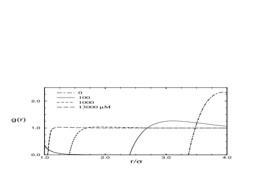
Figure 7: RMSA results for g(r) for $\phi=0.01$, and for various amounts of added 1–1 electrolyte. Other parameters as in Fig. 1.. Full line: two–body mobility function $-8\pi\eta a^{3}\left[\alpha^{rr}_{11}(r)+2\beta^{rr}_{11}(r)\right]$ as in Fig. 1.

Going beyond the EHS model, we can learn more about the ionic strength dependence of $H^{r}_{s}$ by considering Fig. 7, which shows RMSA results for $g(r)$ for a suspension of volume fraction $\phi=0.01$ and various amounts of added electrolyte. The $g(r)$ of the deionized suspension has pronounced oscillations, indicating strong particle correlations. These oscillations become damped out as electrolyte is added, and the peak position $r_{m}$ is shifted towards smaller values. For the system under consideration, very large amounts of electrolyte (i.e. $n_{s}\gg 13mM$) are needed to reach the hard–sphere limit, where the RMSA–$g(r)$ becomes equal to the corresponding Percus–Yevick solution [12]. Consider, e.g., the case $n_{s}=13mM$ in Fig. 7, which corresponds to $\kappa\sigma\simeq 33$ and $\beta u(r=\sigma^{+})\simeq 6.0$. The value of the pair potential at contact distance is still large enough to create a small but non–negligible correlation hole with zero probability of finding another particle. In fact, it is well known [6, 8, 9] that the value of $H^{r}_{s}$, and hence the value of $D^{r}_{s}$, is extremely sensitive to the behaviour of the radial distribution function near touching. This is clearly seen from the fast decay of the two–body scalar mobility function $-8\pi\eta a^{3}\left[\alpha^{rr}_{11}(r)+2\beta^{rr}_{11}(r)\right]$ shown in Fig. 7.

The scaling property $r_{m}\propto\phi^{-\frac{1}{3}}$ is invalid for larger amounts of electrolyte, when the particle diameter becomes a second physically relevant length scale besides the mean particle distance $\bar{r}$. The behaviour of $H^{r}_{s}(\phi)$ at small $\phi$ changes then gradually with increasing $n_{s}$ from a quadratic to a linear $\phi$–dependence. At very large $n_{s}\gg 10mM$, $g(r)$ exhibits only tiny changes in its form when $\phi$ is increased. Hence $H^{r}_{s}$ gets more and more independent of $\phi$, and $H^{r}_{s}(\phi)=1+H^{r}_{s1}(\phi)\phi+\mathcal{O}(\phi^{2})$ becomes linear in $\phi$. A deficiency of our calculations is the fact that we do not obtain the exact hard–sphere result $\left(H^{r}_{s1}\right)_{HS}=-0.630$ in the limit $n_{s}\rightarrow\infty$. Instead the limiting value $\left(H^{r}_{s1}\right)_{HS}=-0.578$ is reached, since we use a series expansion up to terms of order $r^{-20}$ in calculating $H^{r}_{s1}$. However, this truncated expansion is sufficiently good for charge–stabilized suspensions with moderate amounts of added electrolyte, where $x>1.5$ holds (cf. [8, 10]).

6 Conclusions

In the present work, we have investigated the combined effects of electrostatic interactions and hydrodynamic interactions on the short–time rotational diffusion coefficient $D^{r}_{s}$ in monodisperse suspensions of charge–stabilized colloidal particles.

On the basis of the one–component macrofluid model, which neglects electroviscous effects arising from the dynamic distortion of the electric double layer around a particle, we have calculated $H^{r}_{s}=D^{r}_{s}/D^{r}_{0}$ for various systems as a function of volume fraction, effective particle charge, and ionic strength. For these calculations we have used a rooted cluster expansion derived by Degiorgio et. al. [6], combined with far–field expansions of the two–body and three–body mobility functions. We have given evidence that this is a good and well founded approximation in case of charge–stabilized suspensions, as long as the amount of added electrolyte is not very large.

The short–time rotational diffusion of charged particles is less affected by the HI than the rotational diffusion of the uncharged ones. For deionized suspensions of highly charged particles we have found a quadratic volume fraction dependence of the form $H^{r}_{s}=1-a_{r}\phi^{2}$, with a coefficient $a_{r}\simeq 1.15$, which is nearly system independent. The quadratic $\phi$–dependence extends up to rather large volume fractions due to the fact that the leading three–body term is essentially cancelled by the two–body contributions of $\mathcal{O}(r^{-8})$. We have further shown that the qualitative behaviour of $H^{r}_{s}$ can be understood in the framework of a simplified EHS model.

Incidently, dilute deionized suspensions are peculiar also with respect to the $\phi$–dependence of the translational short–time self–diffusion coefficient $D^{t}_{s}$. For this quantity, one obtains a non–analytic concentration dependence of the form $D^{t}_{s}/D^{t}_{0}=1-a_{t}\phi^{4/3}$, with $a_{t}\simeq 2.5$ [14]. The fractal exponent $4/3$ follows also from the EHS model applied to translational self–diffusion.

Upon addition of salt, the quadratic $\phi$–dependence of $D^{r}_{s}$ changes gradually to a $\phi$–dependence typical for hard spheres, where the term linear in $\phi$ dominates for $\phi<0.1$. Very large amounts of salt are required for the systems investigated in this work to reach the hard–sphere limit. This finding is due to the fast decay of the two–body mobility functions with increasing $r$, which renders the two–body term $H^{r}_{s1}$ extremly sensitive to distances close to the contact distance of two particles.

Degiorgio et. al. [6] report a small increase of the measured $D^{r}_{s}$ of hard spheres at the freezing transition where $\phi_{f}=0.49$. The theoretical argument to explain this enhancement is the slightly increased free volume per particle in the crystal phase. The resulting slightly increased interparticle distance turns the HI somewhat less important. We expect that a similar effect should occur for the freezing transition in charge–stabilized suspensions, which occurs at much smaller $\phi$. In our calculations we have used pair distribution functions $g(r)$ calculated with a method (RMSA) designed only for the fluid phase. Therefore, we can not account for the effect of the freezing transition on the short–time rotational diffusion. Nevertheless, we anticipate that our calculations give reasonable results even for the colloidal crystal phase, since our arguments concerning the scaling property of the peak position $r_{m}$ of $g(r)$ should also apply to the crystal phase. Beside that we have shown that $H^{r}_{s}$ is not very sensitive on the details of the shape of $g(r)$ near $r_{m}$. For these reasons, we expect only a small decrease of the coefficient $a_{r}$ at the freezing transition. Therefore we have shown in this paper calculations of $H^{r}_{s}$ up to moderatly large $\phi$, although we know from the Hansen–Verlet criterion that the systems studied here should be crystalline already at small $\phi$.

To our knowledge no experimental or computer simulation data of $D^{r}_{s}$ for deionized charge–stabilized suspensions have been published so far. Because of the interesting differences in the rotational diffusion between suspensions of charged and uncharged particles, it would be worth to check the general predictions of our calculations against experiments and computer simulations. We finally mention that recent DDLS measurements of $D^{r}_{s}$ in deionized suspensions of charged fluorinated polymer particles, initiated by our work, compare favorable with our calculations [13].

Figures

Figure 1: RMSA results for the radial distribution function g(r), modelling deionized suspensions at various volume fractions $\phi$, as indicated in the figure. System parameters are: $\sigma=900\mbox{\AA}$, $Z=500$, $\epsilon=87.0$, $T=294\mbox{K}$, and $n_{s}=0$. The full line is the graph of the two–body scalar mobility function $-8\pi\eta a^{3}\left[\alpha^{rr}_{11}(r)+2\beta^{rr}_{11}(r)\right]$, including terms up to $\mathcal{O}(r^{-20})$ (cf. Eq. (16)).

Figure 2: Results for the normalized short–time rotational self–diffusion coefficient $H^{r}_{s}=D^{r}_{s}/D^{r}_{0}$ for deionized systems, in comparison with the corresponding hard–sphere result of Degiorgio et. al. [6]. Best fit has quadratic $\phi$–dependence: $H^{r}_{s}=1-1.15\phi^{2}$. System parameters as in Fig. 1.

Figure 3: Normalized short–time rotational self–diffusion coefficient $H^{r}_{s}$ for various values of the effective charge $Z$. All system parameters besides $Z$ as in Fig. 1.

Figure 4: Typical RMSA–g(r) (dashed line), and corresponding radial distribution function $g_{EHS}(r)$ of the effective hard–sphere (EHS) model with $2a_{EHS}=r_{m}$. Note the scaling property $r_{m}\propto\phi^{-1/3}$, valid for deionized suspensions.

Figure 5: Dependence of $H^{r}_{s}$ on various two–body contributions, and on the leading three–body contribution. The various cases are indicated in the figure. Parameters as in Fig. 1.

Figure 6: Volume fraction dependence of $H^{r}_{s}$ for various amounts of added 1–1 electrolyte, as indicated in the figure. System parameters as in Fig. 1.

References

- [1] P. N. Pusey, In “Liquids, Freezing and Glass Transition: II”, pp. 763-942, Les Houches Sessions 1989, edited by J.-P. Hansen, D. Levesque, and J. Zinn-Justin, editors, North Holland, Amsterdam, 1991.
- [2] W. Hess and R. Klein, Adv. Phys., 32, 173 (1983).
- [3] R. B. Jones and P. N. Pusey, Annu. Rev. Phys. Chem., 42, 137 (1991).
- [4] G. Nägele, Phys. Rep., in press (1996).
- [5] V. Degiorgio, R. Piazza, and T. Bellini, Adv. Coll. Int. Sci., 48, 61 (1994).
- [6] V. Degiorgio, R. Piazza, and R. B. Jones, Phys. Rev. E, 52, 2707 (1995).
- [7] B. J. Berne and R. Pecora, Dynamic Light Scattering, John Wiley & Sons, New York, 1976.
- [8] R. B. Jones, Physica, A 150, 339 (1988).
- [9] B. Cichocki and B. U. Felderhof, J. Chem. Phys., 89, 1049 (1988).
- [10] R. B. Jones and R. Schmitz, Physica, A 149, 373 (1988).
- [11] G. Nägele, M. Medina-Noyola, R. Klein, and J. L. Arauz-Lara, Physica, A 149, 123 (1988).
- [12] J.-P. Hansen and I. R. McDonald, Theory of Simple Liquids, 2nd edition, Academic Press, London, 1986.
- [13] F. Bitzer, T. Palberg, and P. Leiderer, University of Konstanz, private communication.
- [14] G. Nägele, B. Mandl, and R. Klein, Progr. Colloid Polym. Sci, 98, 117 (1995).