Density waves in dry granular media falling through a vertical pipe

Abstract

We report experimental measurements of density waves in granular materials flowing down in a capillary tube. The density wave regime occurs at intermediate flow rates between a low density free fall regime and a high compactness slower flow. We observe this intermediate state when the ratio of the tube diameter and the particles size lies between 6 and 30. The propagation velocity of the waves is constant along the tube length and increases linearly with the total mass flow rate $\rm\Phi$. The wave structures include compact clogs (lengths are independent of $\rm\Phi$) and bubbles of low compactness (lengths increase with $\rm\Phi$). Both length distributions are invariant along the tube length. A model assuming a free fall regime in the bubbles and a compactness of $35\%$ inside the clogs allows to account for the mass distribution in the flow.

1 Introduction

Nowadays dry granular media take up an important place in our life. Scientists have studied these materials to understand its behavior in nature [1]-[17] and for industrial applications [3][4][17]. One of these problems, which we are interested in understanding, is the appearance of density waves in downward flows of granular media inside a pipe [17]. These effects have significant analogies with the traffic flow model that successfully characterizes traffic jams on highways [1]. Several authors have already analyzed the problem [1]-[17]. However, the dependence of the structure of the waves on the physical parameters controlling the flow have not been studied systematically in these works. In the present letter we study in particular the evolution of the characteristic geometry of the waves and of its propagation velocity in relation to the total mass flow rate.

2 Experimental setup

The experimental setup (Fig.1) comprises a conical hopper with an opening angle of 60 degrees attached to a vertical glass pipe of a length of 1.3 m and an internal diameter of approximately 2.9 mm. At the bottom of the pipe a variable closure of the outlet makes it possible to adjust the outflow. With an optical acquisition device we analyze variations of the grain packing fraction. Light of a standard 50 Watt halogen lamp falls onto a double slit which divides the light in two beams and then a lens concentrates the light beams onto the pipe as two narrow horizontal lines. Another lens refocuses the light scattered and diffracted by the falling grains and the pipe itself onto two light detection diodes on the other side. The high sensitivity of the diodes makes it indispensable to protect the optical axis from stray radiation. Using two light beams allows to determine the average velocity of the density waves. We define two measurement heights, $\rm h_{1}$ in the vicinity of the top (20 cm below the hopper) and $\rm h_{2}$ near the bottom of the pipe (30 cm above the outlet), to study the dependence of the variations of the grain density on the length of the pipe. Simultaneously with the optical acquisition we measure the mass flow as a function of the time by adding electronic computer controlled scales under the outlet of the pipe. The time variations of the transmitted light corresponding to the various measured parameters are recorded and processed afterwards on a Unix Workstation.
We performed our experiments with small glass beads of a average diameter of 200 $\rm\mu m$ and small glass splinters of a mean size between 90 and 200 $\rm\mu m$.

3 Qualitative observations

Before performing the experiments, it is important to avoid excess humidity in the granular materials, else strong adhesive forces arise between the grains and between grains and pipe. Simply blowing into the pipe creates enough humidity that the pipe can only be used again after drying it with hot air.
The observed phenomena can be subdivided in three regimes:
The first and simplest case describes the behavior of grains falling down a pipe without or with only a small outlet closure: this case corresponds to the largest mass flow rates. When grains fall down from the hopper they drag air with them inducing suction. In the mentioned case of largest mass flow rates this suction causes air to flow through the sand in the upper part of the pipe. To verify this a balloon filled with air was put over the hopper. Due to the suction the balloon contracted.
The second regime is characterized by a high compactness of the flowing grains which is approximately constant over the length of the pipe. This case corresponds to the lowest flow rate values (small outlet opening).
Between the two cases mentioned above we observe a third regime characterized by density waves. Each individual density wave consists of two different parts. The first highly compact and dense section will be called a “clog”. The second is a bubble filled with air in which the particle density is lower and their velocity higher. When the outflow is reduced from the free fall case a plug builds up at the bottom of the pipe. In this case the air stream from the top to the bottom is hindered by the plug. This assumption could also be verified with an air-balloon. The contraction of the balloon caused by the suction in the free fall regime discussed above stops immediately with the formation of the plug at the bottom of the pipe.
Fig.2 illustrates a typical density wave of particles. The radial structure of the bubbles has been determined by video analysis.
To obtain the density waves it is necessary to keep the ratio rat of the diameter of the fixed pipe and the size of the particles within certain limits. We have verified in several experiments the condition:

$$\rm 30\geq rat\geq 6.$$ (1)

For $\rm rat>30$ we always obtain the free fall regime. For $\rm rat<6$ only the compact regime is observed and the flow very often stops completely due to arching.
We have noticed that density waves do not appear directly at the hopper outlet but at a certain distance $\rm\Delta$ below. The distance $\rm\Delta$ increases with grain size.

4 Analysis of density variations using light transmission

As mentioned above we analyze the time variations of the intensity of light transmitted through the pipe. Considering typical variation in the regime of density waves the high intensity peaks correspond to air bubbles and the intervals between the peaks represent clogs. To extract information from these time series we have introduced a threshold distinguishing between high (clogs) and low (air bubbles) compactness. We have chosen this threshold value just large enough to eliminate the influence of the noise of the base line as one can see in Fig.3.
We obtain a binary curve by replacing the data points above the threshold by one and the others by zero. In this way we introduce for each individual bubble and clog labeled i the respective characteristic transit times $\rm\tau_{x}^{i}$ and $\rm\tau_{l}^{i}$. They are defined as the time during which the measured signal remains respectively higher or lower than the threshold when the bubble or the clog moves through the measurement section. Plotting the different characteristic transit times as a function of time leads to histograms. The histogram of the duration of the clogs displays a well defined peak corresponding to the average transit time $\rm\tau_{l}$ of the clogs. In contrast the transit time distribution of the bubbles is much broader, so that we obtain $\rm\tau_{x}$ by averaging over all $\rm\tau_{x}^{i}$. Fig.4 shows some typical histograms. We have superimposed two measurements performed at two different heights with approximately the same mass flow. We observe the changes with distance of the histograms are extremely small: this implies that the granular flow has reached a stationary regime even at the upper measurement level.
Measurements using two light beams displaced a distance D on the axis of the pipe (Fig.1) lead to two similar time series, shifted a time $\rm\tau_{D}$ representing the transit time of the density variations between the two measurement sections. From the peak of the correlation function of the two time series we obtain $\rm\tau_{D}$ and thus the apparent velocity $\rm v_{l}=D/\tau_{D}$ of the clogs. In table 1 and 2, concerning the different measurement heights $\rm h_{1}$ and $\rm h_{2}$, one can see the relations between $\rm\tau_{l},\,\tau_{x},\,\tau_{D}$ and the total mass flow $\rm\Phi$. Furthermore we see also the relation between the transit times, the velocity $\rm v_{l}$ and the calculated values for the respective lengths x of the bubbles and l of the clogs. The plot of the global mass flow rate $\rm\Phi$ as a function of $\rm v_{l}$ in Fig.5 shows an almost linear increase of $\rm\Phi$ with $\rm v_{l}$, so that we can write:

$$\rm\Phi=\Phi_{0}+A\,v_{l}.$$ (2)

We obtain that $\rm A=4.9\,g/m$ and $\rm\Phi_{0}=1.2\,g/s$.
We estimate the characteristic length l of the clogs from their velocity and transit time,

$$\rm l=v_{l}\,\tau_{l}.$$ (3)

In Fig.5 we have superimposed two series of measurements performed at two different measurement heights $\rm h=h_{1}$ and $\rm h=h_{2}$. We observe that the velocity $\rm v_{l}$ is independent of the measurement heights h and therefore we assume that $\rm v_{l}$ is constant along the pipe. We calculate the average length x of the low particle density bubbles from the mean transit time $\rm\tau_{x}$ of a bubble through a light beam.

$$\rm v\simeq v_{l}=const,$$

$$\rm\frac{l}{\tau_{l}}=\frac{x}{\tau_{x}}.$$ (4)

Eq.(4) leads to

$$\rm x=l\,\frac{\tau_{x}}{\tau_{l}}.$$ (5)

Fig.6 illustrates the relation between l, x and the global mass flow rate $\rm\Phi$. The two different kinds of symbols represent the two different measurement heights mentioned above.
As can be seen in Fig.6 the length l of the clogs is nearly independent of both the mass flow rate and the height at which the density measurement is performed. In contrast, the average length x of the air bubbles varies. We observe at both the higher and lower measurement height an almost linear increase of x with $\rm\Phi$.
After computing the respective lengths l and x it is possible to obtain the mean masses $\rm m_{l}$ and $\rm m_{x}$ of the granular material in a clog and in a bubble. In order to estimate $\rm m_{l}$ we have measured independently the total mass $\rm m_{p}$ of the grains filling completely the full length $\rm L_{p}$ of the pipe under zero flow conditions. $\rm m_{l}$ verifies:

$$\rm m_{l}=\frac{m_{p}}{L_{p}}\,l\,\frac{c(\Phi)}{c_{0}}.$$ (6)

The variable $\rm c(\Phi)$ represents the compactness of the grain packing in the flowing clogs and $\rm c_{0}$ in a non flowing packing corresponding to the mass $\rm m_{p}$ (experimentally, one finds: $\rm c_{0}\approx 0.63$).
In the next step we calculate the mean mass $\rm m_{x}$ of a low density pocket. Let us consider now the mass flow rate of grains $\rm\Phi_{v,g}$ in an inertial frame moving at the velocity $\rm v_{l}$ of the clog. The density wave structure in this reference frame is stationary. This assumption results in a total mass flow rate $\rm\Phi$ in the fixed reference laboratory frame of

$$\rm\Phi=\Phi_{v,g}+\Phi_{v,l},$$ (7)

with

$$\rm\Phi_{v,l}=\frac{m_{x}+m_{l}}{\tau_{x}+\tau_{l}}=v_{l}\,\frac{m_{x}+m_{l}}{x+l}.$$ (8)

The initial velocity $\rm v_{0,g}$ of the grains at the top of an air bubble in the moving reference frame is assumed to verify

$$\rm v_{0,g}=\frac{\Phi_{v,g}}{\pi\,r^{2}\,\rho_{g}\,c(\Phi)}=\frac{\Phi_{v,g}}{K\,c(\Phi)},$$ (9)

with

$$\rm K=\pi\,r^{2}\,\rho_{g},$$ (10)

$\rm\rho_{g}$ is the bulk density of the glass used for the grains. Equation (9) implies that both the grain concentration and their velocity are continuous at the bottom of the clogs. The unknown variables are $\rm m_{x}$, $\rm\Phi_{v,g}$ and $\rm c(\Phi)$. We assume that the grains in an air bubble fall freely and the interactions between the grains and the particles of the wall are negligible, so that

$$\rm\frac{dv_{g}}{dt}=g.$$ (11)

The grain velocity $\rm v_{g}$ in the reference moving frame is related to $\rm\Phi_{v,g}$,

$$\rm\Phi_{v,g}=\rho(z)\,v_{g}(z),$$ (12)

in which $\rm\rho(z)$ is the integration of the local mass density over the cross section at height z. One obtains the mass of particles $\rm m_{x}$ inside a bubble using relations (11) and integrating $\rm\rho(z)$ from 0 to x to compute the grain mass density:

$$\rm m_{x}=\int_{0}^{x}\rho(z)\,dz=\frac{\Phi_{v,g}^{2}}{g\,K\,c(\Phi)}\,(\sqrt{1+\frac{2\,x\,g\,K^{2}\,c^{2}(\Phi)}{\Phi_{v,g}^{2}}}-1).$$ (13)

Inserting Eq.(13) into Eq.(7) leads to

$$\rm\Phi=\Phi_{v,g}+\frac{v_{l}}{x+l}\left(\frac{m_{p}}{L_{p}}\,l\,\frac{c(\Phi)}{c_{0}}+\frac{\Phi_{v,g}^{2}}{g\,K\,c(\Phi)}\left(\sqrt{1+\frac{2\,x\,g\,K^{2}\,c^{2}(\Phi)}{\Phi_{v,g}^{2}}}-1\right)\right).$$ (14)

We solve Eq.(14) numerically to obtain $\rm\Phi_{v,g}$ under the assumption $\rm c(\Phi)=const$. We used the criterion that when $\rm v_{l}=0$ the total flux equals the grain flow rate, i.e.,

$$\rm\Phi(v_{l}=0)=\Phi_{v,g}(v_{l}=0),$$ (15)

to obtain $\rm c(\Phi)$= 0.35. We see in table 3 and 4, corresponding to the different measurement heights $\rm h_{1}$ and $\rm h_{2}$, that $\rm\Phi_{v,g}$ and $\rm\Phi_{v,l}$ increase with the velocity $\rm v_{l}$, but $\rm\Phi_{v,l}$ remains for each value of the velocity under $50\%$ of the value of $\rm\Phi_{v,g}$. We have illustrated these relations in Fig.5. The upper line corresponds to the total mass flow rate and the others correspond to $\rm\Phi_{v,g}$ and $\rm\Phi_{v,l}$.
Replacing $\rm\Phi_{v,g}$ in Eq.(13) gives us the masses $\rm m_{x}$ for the measurement heights $\rm h_{1}$ and $\rm h_{2}$. Decreasing the total mass flow rate $\rm\Phi$ leads to an approach of the masses $\rm m_{x}$ and $\rm m_{l}$. This behavior is consistent with the lengths of the bubbles and the clogs as one can see in Fig.6.

5 Conclusion

In the present letter we have verified the existence of a regime of density waves in dry granular media at intermediate flow rates between a low density free fall regime and a slow regime of flow of high compactness. We obtain nearly stationary structures of waves including compact clogs and bubbles of low compactness. Both the length distributions of clogs and bubbles and the propagation velocity of the waves are constant along the pipe. The lengths of the clogs are independent of the total mass flow rate $\rm\Phi$. However, the lengths of the bubbles increase with $\rm\Phi$ and they are a factor 1.5 to 3 larger than the clog lengths. A model assuming a free fall inside the bubbles and a compactness of $35\%$ inside the clogs well reproduces the mass distribution in the flow.
It is clear that there are still numerous problems which have to be solved. A key issue for the full understanding of the phenomena will be the determination of the forces acting on the grains both in the clog and bubble zones. This includes considering friction forces between the grains and the walls and further hydrodynamic forces resulting from the gas in the column. A crucial point will be the determination and prediction of the pressure gradients in the column.

Acknowledgment

The authors thank gratefully S. Schwarzer and H. Puhl for a critical reading of the manuscript.

independence of the measurement height. Assuming that the compactness

Figures

• Figure 1: Experimental Setup.
  

• Figure 2: Schematic view of density waves formed by particles.
  

• Figure 3: Typical time variation of the intensity of light transmitted through the pipe with defined threshold to distinguish between high and low compactness ($\rm\Phi=1.980$ g/s).
  

• Figure 4: Histograms of time for clogs and air bubbles in a semi-log plot. The continuous lines correspond to the measurement height $\rm h_{2}$, with $\rm\Phi(h_{2})=2.466$ g/s. The dotted lines correspond to the measurement height $\rm h_{1}$, with $\rm\Phi(h_{1})=2.459$ g/s.
  

• Figure 5: Total mass flow as a function of measured clog velocity along the pipe. The triangles correspond to the measurement height $\rm h_{1}$ and the checks to the measurement height $\rm h_{2}$.
  

• Figure 6: Characteristic lengths of clogs (lower values) and air bubbles (upper values) as a function of the mass flow. The triangles correspond to the measurement height $\rm h_{1}$ and the checks to the measurement height $\rm h_{2}$.
  

Tables

• Table 1: $\rm\tau_{l},\,\tau_{x},\,\tau_{D},\,v_{l},\,x,\,l$ as a function of the total mass flow $\rm\Phi$ (measurement height $\rm h_{1}$).
  

• Table 2: $\rm\tau_{l},\,\tau_{x},\,\tau_{D},\,v_{l},\,x,\,l$ as a function of the total mass flow $\rm\Phi$ (measurement height $\rm h_{2}$).
  

• Table 3: $\rm\Phi,\,\Phi_{v,g},\,\Phi_{v,l},\,v_{l},\,m_{l},\,m_{x}$ (measurement height $\rm h_{1}$).
  

• Table 4: $\rm\Phi,\,\Phi_{v,g},\,\Phi_{v,l},\,v_{l},\,m_{l},\,m_{x}$ (measurement height $\rm h_{2}$).
  

Figure 1:

Figure 2:

Figure 3:

Figure 4:

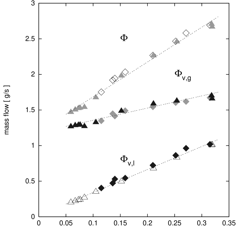
Figure 5:

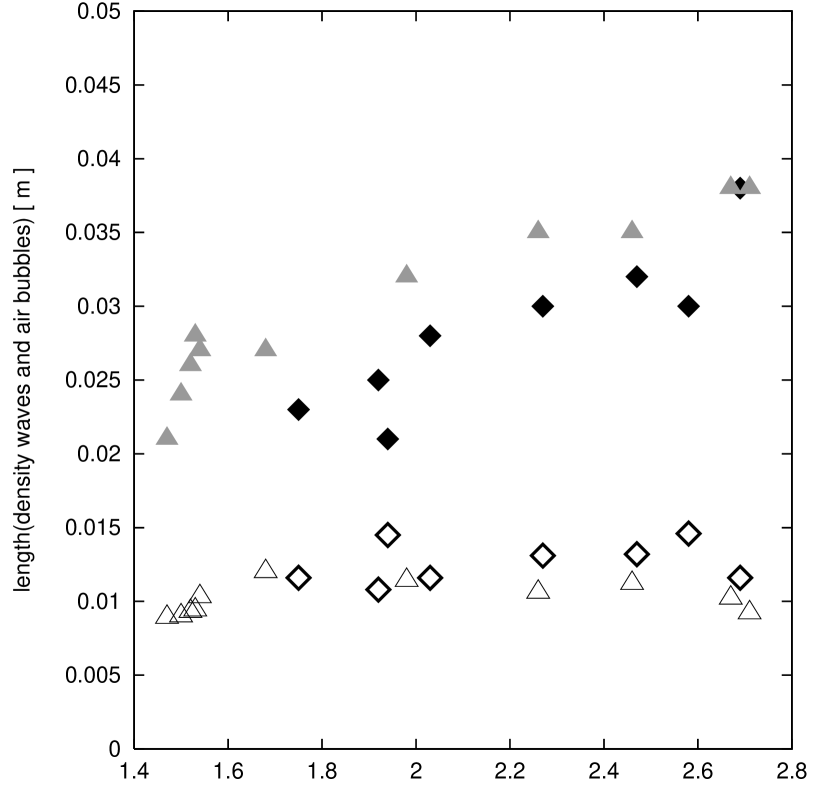
Figure 6:

$\rm\Phi\,[g/s]$	2.67	2.71	2.46	2.26	1.98	1.68	1.54	1.53
$\rm\tau_{l}\,[ms]$	32.09	28.89	44.22	50.42	75.24	114.24	122.22	123.75
$\rm\tau_{x}\,[ms]$	118.81	118.75	136.38	167.75	212.96	260.77	317.51	369.28
$\rm\tau_{D}\,[ms]$	59.56	59.75	74.80	90.05	13	180.95	226.19	250
$\rm v_{l}\,[m/s]$	0.319	0.318	0.254	0.211	0.152	0.105	0.084	0.076
$\rm x\,[m]$	0.038	0.038	0.035	0.035	0.032	0.027	0.027	0.028
$\rm l\,[m]$	0.010	0.009	0.011	0.011	0.011	0.012	0.010	0.009

Table 1:

$\rm\Phi\,[g/s]$	2.69	2.58	2.47	2.27	2.03	1.94	1.92	1.75
$\rm\tau_{l}\,[ms]$	36.70	53.86	52.56	62.48	72.86	103.35	79.04	101.05
$\rm\tau_{x}\,[ms]$	120.07	110.77	125.31	144.15	177.91	152.75	188.43	199.71
$\rm\tau_{D}\,[ms]$	60.32	70.11	75.40	90.48	119.50	135.71	139.71	165.22
$\rm v_{l}\,[m/s]$	0.315	0.271	0.252	0.210	0.159	0.140	0.136	0.115
$\rm x\,[m]$	0.038	0.030	0.032	0.030	0.028	0.021	0.025	0.023
$\rm l\,[m]$	0.012	0.015	0.013	0.013	0.012	0.015	0.011	0.012

Table 2:

$\rm\Phi\,[g/s]$	2.67	2.71	2.46	2.26	1.98	1.68	1.54	1.53
$\rm\Phi_{v,g}\,[g/s]$	1.66	1.70	1.63	1.59	1.49	1.33	1.27	1.29
$\rm\Phi_{v,l}\,[g/s]$	1.01	1.01	0.83	0.68	0.50	0.35	0.27	0.24
$\rm v_{l}\,[m/s]$	0.319	0.318	0.254	0.211	0.152	0.105	0.084	0.076
$\rm m_{l}\,[g]$	0.052	0.047	0.057	0.054	0.058	0.061	0.052	0.048
$\rm m_{x}\,[g]$	0.101	0.103	0.094	0.093	0.084	0.069	0.067	0.070

Table 3:

$\rm\Phi\,[g/s]$	2.69	2.58	2.47	2.27	2.03	1.94	1.92	1.75
$\rm\Phi_{v,g}\,[g/s]$	1.67	1.62	1.60	1.54	1.49	1.42	1.45	1.35
$\rm\Phi_{v,l}\,[g/s]$	1.02	0.96	0.86	0.72	0.54	0.53	0.47	0.40
$\rm v_{l}\,[m/s]$	0.315	0.271	0.252	0.210	0.159	0.140	0.136	0.115
$\rm m_{l}\,[g]$	0.059	0.074	0.067	0.066	0.059	0.074	0.055	0.059
$\rm m_{x}\,[g]$	0.102	0.085	0.088	0.082	0.077	0.061	0.070	0.063

Table 4:

References

- [1] K. Nagel and M. Schreckenberg, J. Physique I 2, 2221 (1992)
- [2] T. Musha and H. Higuichi, Jap. J. Appl. Phys. 15, 1271 (1976)
- [3] M.J. Lighthill and G.B. Witham, Proc. Roy. Soc. A 229, 281 and 317 (1955); M. Leibig, Phys. Rev. E 49, 184 (1994)
- [4] G.W. Baxter, R.P. Behringer, T. Fagert and G.A. Johnson, Phys. Rev. Lett. 62 2825 (1989)
- [5] 8 G.W. Baxter, R.P. Behringer, Phys. Rev. A 42 1017 (1990)
- [6] G. Peng and H.J. Herrmann, Phys. Rev. E 49 R1796 (1994)
- [7] H.M. Jaeger and S.R. Nagel, Science 255 1523 (1992)
- [8] T. Pöschel, J. Physique I 4, 499 (1994)
- [9] D.C. Hong, S. Yue, J.K. Rudra, M.Y. Choi and Y.W. Kim, Phys. Rev. E 50 4123 (1994)
- [10] Y-h. Taguchi, Phys. Rev. Lett. 69 1367 (1992)
- [11] H.M. Jaeger, C-h. Liu and S.R. Nagel, Phys. Rev. Lett. 62 40 (1989)
- [12] J.A. Gallas, H.J. Herrmann and S. Sokolowski, Phys. Rev. Lett. 69 1371 (1992)
- [13] T. Pöschel and H.J. Herrmann, Physica A 198, 441 (1993)
- [14] J. Lee and H.J. Herrmann, J. Phys. A 26, 373 (1993)
- [15] P. Bak, C. Tang and K. Wiesenfeld, Phys. Rev. Lett. 59 381 (1987)
- [16] P.Evesque and J. Rajchenbach, Phys. Rev. Lett. 61 44 (1989)
- [17] C.K.K. Lun and S.B. Savage and D.J. Jeffrey and N. Chepurni, J.F.M. 140 223 (1984)