Distribution of the Absorption by Chaotic States in Quantum Dots

Abstract

The mesoscopic fluctuations of the absorption at optical transitions from a low energy regular state to high energy chaotic states in an aggregate of semiconductor quantum dots is studied. We provide a universal dependence of the distribution of the absorption coefficient on the total number of dots and the ratio of the level broadening to the level spacing. The distribution remain broad even at large broadening, and the absorption spectrum should demonstrate a strong sensitivity to weak magnetic field in the region of large and weak absorption. The results can also apply to the absorption of Rydberg atoms in strong magnetic field at the pre-threshold ionization.

Semiconductor quantum dots are now a subject of intensive study as potential devices with controlled optical properties [1, 2]. Because of restricted geometry, their spectra are discrete and are modified by variation of the dot size. The experimental absorption spectrum demonstrates a good agreement with theoretical calculations for optical transitions between the first few size-quantized levels [3, 4]. For these low energy states, fluctuations of the dot size give broadening to observed transitions, but their levels remain still well identified. Fluctuations of the confinement potential play no prominent role since the corresponding electron wave length is of the order of the dot size, i.e., exceeds a length scale of these irregularities. For sufficiently high energy states whose wave lengths amount to an atomic scale or a characteristic scale of fluctuations, their levels and wavefunctions are determined by such ‘imperfections’ of the confinement potential. The size of the dot controls only the average interlevel spacing. The confinement part fluctuates from dot to dot and even for a given dot wavefunctions of such high energy states changes unpredictedly from level to level. This allows us to take the statistical description for the high energy chaotic states.

In the present paper, we study the absorption coefficient for the transitions from a given initial state into these high energy chaotic states. The initial state can be the ground state or a low energy state as well as a local electronic state, e.g., at the donor inside the dot. For an aggregate of dots, the experimental absorption spectrum should show featureless background with rare high peaks and the weak absorption regions. Our result describes the statistics of these fluctuations. We have found that the amplitude of fluctuations in the absorption depends strongly on the total number of dots, and also on the ratio of the level broadening to the level spacing. When the latter is small, the fluctuation of absorption spectra becomes highly asymmetric, demonstrating abrupt decay for small ones and slow power-law decay for large fluctuations. The fluctuations remain appreciable even when the broadening is much larger than the level spacing and therefore the fluctuations should be still observable for an ensemble of finite number of dots.

Similarly to the statistics of energy levels [5] and wavefunctions in chaotic systems [6, 7], the distribution function for the absorption coefficient manifests the universal behavior which is determined only by the generic symmetry of the system [8]. In the absence of the spin-orbit interaction, there are two universality classes present: the orthogonal class for time-reversal-invariant (T-invariant) systems ($\beta=1$), and the unitary class for time-reversal-breaking (T-breaking) systems ($\beta=2$). The crossover between these two universality classes will occur with the magnetic flux $\phi$ through a dot around $\phi\sim h/e\sqrt{g}$ where $g$ is the dimensionless conductance [9]. We investigate the statistics of the absorption for both universality classes.

Analogous absorption spectrum should be observed for Rydberg atoms in a high magnetic field where the pre-ionization states are considered chaotic [10].

Consider the absorption for a single dot at optical transition from a given initial state $|{\Phi_{0}}\rangle$ with the energy $E_{0}$ to excited states $|\psi_{n}\rangle$ with energy $E_{n}$, which we assume fully chaotic. Under the resonance, the real part of the polarizability $\alpha$ is negligible, so $\alpha(\Omega)$ becomes

$$\alpha(\Omega)\approx i\pi\sum_{n}|P_{n0}|^{2}\;\delta_{\Gamma}(\Omega-\Omega_{n}),$$ (1)

where $\Omega_{n}=E_{n}-E_{0}$, and $P_{n0}=\langle\psi_{n}|\hat{P}|\Phi_{0}\rangle$, the transition dipole matrix element. The explicit form of the transition dipole $\hat{P}$ is not needed to proceed the following argument. $\delta_{\Gamma}$ is a $\delta$-function with a finite broadening $\Gamma$, defined by $2\pi\delta_{\Gamma}(E)\equiv{\Gamma/(E^{2}+\Gamma^{2}/4})$. A basic assumption here is that the level width is fixed among these high energy excited states. Since such broadening is dominated mainly by electron escape into the host matrix and an electron can leave a dot through its whole boundary, fluctuations of level widths should be suppressed.

The absorption (extinction) coefficient $\kappa$ in this regime is determined by

$$\kappa(\Omega)=\sqrt{2\pi|\alpha(\Omega)|}.$$ (2)

Reflecting random nature of $\Omega_{n}$ and chaotic wavefunctions, $\alpha(\Omega)$ and $\kappa(\Omega)$ become highly fluctuating quantities, either from sample to sample or by slightly changing $\Omega$. To examine these statistical properties, we will investigate the following the probability distribution functions:

$${\cal P}(x;\{\alpha\})=\left\langle\delta(x-\alpha(\Omega)/\alpha_{0})\right\rangle,$$ (4)

$${\cal P}(x;\{\kappa\})=\left\langle\delta(x-\kappa(\Omega)/\kappa_{0})\right\rangle,$$ (5)

where $\alpha_{0}$ and $\kappa_{0}$ are the average values of $\alpha$ and $\kappa$, respectively (see Eq.(11) below). We obtain the analytical expressions of ${\cal P}(x;\{\kappa\})$ and ${\cal P}(x;\{\alpha\})$, both for T-invariant and T-breaking systems.

We proceed this task by connecting the distribution functions of $\alpha$ or $\kappa$ with that of the local density of states $\nu(\mathchoice{{\hbox{\boldmath$\displaystyle r$}}}{{\hbox{\boldmath$\textstyle r$}}}{{\hbox{\boldmath$\scriptstyle r$}}}{{\hbox{\boldmath$\scriptscriptstyle r$}}})$ defined by

$$\nu(\mathchoice{{\hbox{\boldmath$\displaystyle r$}}}{{\hbox{\boldmath$\textstyle r$}}}{{\hbox{\boldmath$\scriptstyle r$}}}{{\hbox{\boldmath$\scriptscriptstyle r$}}},E)=\sum_{n}|\psi_{n}(\mathchoice{{\hbox{\boldmath$\displaystyle r$}}}{{\hbox{\boldmath$\textstyle r$}}}{{\hbox{\boldmath$\scriptstyle r$}}}{{\hbox{\boldmath$\scriptscriptstyle r$}}})|^{2}\delta_{\Gamma}(E-E_{n}),$$ (6)

$${\cal P}(x;\{\nu\})=\left\langle{\delta(x-\nu(\mathchoice{{\hbox{\boldmath$\displaystyle r$}}}{{\hbox{\boldmath$\textstyle r$}}}{{\hbox{\boldmath$\scriptstyle r$}}}{{\hbox{\boldmath$\scriptscriptstyle r$}}},E)/\nu_{0})}\right\rangle,$$ (7)

where $\nu_{0}=\langle\nu(\mathchoice{{\hbox{\boldmath$\displaystyle r$}}}{{\hbox{\boldmath$\textstyle r$}}}{{\hbox{\boldmath$\scriptstyle r$}}}{{\hbox{\boldmath$\scriptscriptstyle r$}}},E)\rangle$. By utilizing statistical properties of chaotic wavefunctions, we can show that

$${\cal P}(x;\{\alpha\})={\cal P}(x;\{\nu\})\equiv{\cal P}(x),$$ (9)

$${\cal P}(x;\{\kappa\})=2x{\cal P}(x^{2}).$$ (10)

First we show how Eq. (Distribution of the Absorption by Chaotic States in Quantum Dots) was derive. The average of the polarizability become independent of $\Omega$ and is given by

$$\alpha_{0}={i\pi\over\Delta}\>\left\langle\,{|P_{n0}|^{2}}\right\rangle$$ (11)

where $\Delta=1/\nu_{0}V$ is the mean level spacing with the dot volume $V$. $\langle\,{|P_{n0}|^{2}}\rangle$ is the average intensity of the transition dipole moment [11] defined by

$$\left\langle\,{|P_{n0}|^{2}}\right\rangle={1\over V}\int\!\!d\mathchoice{{\hbox{\boldmath$\displaystyle r$}}}{{\hbox{\boldmath$\textstyle r$}}}{{\hbox{\boldmath$\scriptstyle r$}}}{{\hbox{\boldmath$\scriptscriptstyle r$}}}_{1}d\mathchoice{{\hbox{\boldmath$\displaystyle r$}}}{{\hbox{\boldmath$\textstyle r$}}}{{\hbox{\boldmath$\scriptstyle r$}}}{{\hbox{\boldmath$\scriptscriptstyle r$}}}_{2}\,\langle\Phi_{0}|\hat{P}|\mathchoice{{\hbox{\boldmath$\displaystyle r$}}}{{\hbox{\boldmath$\textstyle r$}}}{{\hbox{\boldmath$\scriptstyle r$}}}{{\hbox{\boldmath$\scriptscriptstyle r$}}}_{1}\rangle f(r_{12})\langle\mathchoice{{\hbox{\boldmath$\displaystyle r$}}}{{\hbox{\boldmath$\textstyle r$}}}{{\hbox{\boldmath$\scriptstyle r$}}}{{\hbox{\boldmath$\scriptscriptstyle r$}}}_{2}|\hat{P}|\Phi_{0}\rangle,$$ (12)

with $f(r_{12})\equiv V\left\langle\psi_{n}(\mathchoice{{\hbox{\boldmath$\displaystyle r$}}}{{\hbox{\boldmath$\textstyle r$}}}{{\hbox{\boldmath$\scriptstyle r$}}}{{\hbox{\boldmath$\scriptscriptstyle r$}}}_{1})\psi_{n}^{*}(\mathchoice{{\hbox{\boldmath$\displaystyle r$}}}{{\hbox{\boldmath$\textstyle r$}}}{{\hbox{\boldmath$\scriptstyle r$}}}{{\hbox{\boldmath$\scriptscriptstyle r$}}}_{2})\right\rangle$ to describe spatial correlations of the wavefunction amplitude. To calculate the distribution, we need its higher moments

$$\left\langle{\,|P_{n0}|^{2k}}\right\rangle =\int\prod_{i=1}^{k}\left(d\mathchoice{{\hbox{\boldmath$\displaystyle r$}}}{{\hbox{\boldmath$\textstyle r$}}}{{\hbox{\boldmath$\scriptstyle r$}}}{{\hbox{\boldmath$\scriptscriptstyle r$}}}_{i}d\mathchoice{{\hbox{\boldmath$\displaystyle r$}}}{{\hbox{\boldmath$\textstyle r$}}}{{\hbox{\boldmath$\scriptstyle r$}}}{{\hbox{\boldmath$\scriptscriptstyle r$}}}^{\prime}_{i}\,\left\langle{\Phi_{0}}\right|\hat{P}\left|{\mathchoice{{\hbox{\boldmath$\displaystyle r$}}}{{\hbox{\boldmath$\textstyle r$}}}{{\hbox{\boldmath$\scriptstyle r$}}}{{\hbox{\boldmath$\scriptscriptstyle r$}}}_{i}}\right\rangle\left\langle{\mathchoice{{\hbox{\boldmath$\displaystyle r$}}}{{\hbox{\boldmath$\textstyle r$}}}{{\hbox{\boldmath$\scriptstyle r$}}}{{\hbox{\boldmath$\scriptscriptstyle r$}}}^{\prime}_{i}}\right|\hat{P}\left|{\Phi_{0}}\right\rangle\right)$$ (14)

$$\quad\times\left\langle\psi_{n}(\mathchoice{{\hbox{\boldmath$\displaystyle r$}}}{{\hbox{\boldmath$\textstyle r$}}}{{\hbox{\boldmath$\scriptstyle r$}}}{{\hbox{\boldmath$\scriptscriptstyle r$}}}_{1})\psi_{n}^{*}(\mathchoice{{\hbox{\boldmath$\displaystyle r$}}}{{\hbox{\boldmath$\textstyle r$}}}{{\hbox{\boldmath$\scriptstyle r$}}}{{\hbox{\boldmath$\scriptscriptstyle r$}}}^{\prime}_{1})\cdots\psi_{n}(\mathchoice{{\hbox{\boldmath$\displaystyle r$}}}{{\hbox{\boldmath$\textstyle r$}}}{{\hbox{\boldmath$\scriptstyle r$}}}{{\hbox{\boldmath$\scriptscriptstyle r$}}}_{k})\psi_{n}^{*}(\mathchoice{{\hbox{\boldmath$\displaystyle r$}}}{{\hbox{\boldmath$\textstyle r$}}}{{\hbox{\boldmath$\scriptstyle r$}}}{{\hbox{\boldmath$\scriptscriptstyle r$}}}^{\prime}_{k})\right\rangle.$$

The spatial correlation between the local values of wavefunction exists only within the mean free path $\ell$. Beyond such distance, the wavefunction can be seen to be fluctuating independently. As a result, in the leading order of $\ell\lambda^{d-1}/V$ ($\lambda$ is the wave length), we get

$$\left\langle\,|P_{n0}|^{2k}\right\rangle=\left\langle\,|P_{n0}|^{2}\right\rangle^{k}\;\left\{\begin{array}[]{cc}k!&(\mbox{for }\beta=2)\\ {(2k-1)!!}&{(\mbox{for }\beta=1)}\end{array}\right..$$ (15)

This shows that, as well as $|\psi_{n}(\mathchoice{{\hbox{\boldmath$\displaystyle r$}}}{{\hbox{\boldmath$\textstyle r$}}}{{\hbox{\boldmath$\scriptstyle r$}}}{{\hbox{\boldmath$\scriptscriptstyle r$}}})|^{2}$, the distribution of $|P_{n0}|^{2}$ and equally oscillator strength $f_{n}=2m\Omega_{n}|P_{n}o|^{2}$ are characterized by the the Porter-Thomas distribution [12] after an appropriate rescaling. By comparing Eqs. (1) and (6), we can conclude Eq. (9), then Eq. (10) follows from Eq. (2).

To evaluate ${\cal P}(x)$ analytically, it is convenient to work on its Laplace transformation ${\cal L}(s)$ [13]

$${\cal L}(s)=\int_{0}^{\infty}{dx\,e^{-s\gamma x}\;{\cal P}(x)},$$ (16)

where $\gamma\equiv\pi\Gamma/\Delta$. The averaging for ${\cal L}(s)$ can be decomposed into averaging over eigenfunctions and energy levels, and the former is recasted by the Porter-Thomas distribution. Since the Porter-Thomas distribution depends on the symmetry parameter $\beta$, the result of the integration over eigenfunctions ${\cal L}(s)={\cal L}_{\beta}(s)$ becomes

$${\cal L}_{\beta}(s)\equiv\left\langle\left({{\det[(E-H)^{2}+\Gamma^{2}/4]\over\det[(E-H)^{2}+\tilde{\Gamma}^{2}/4]}}\right)^{\beta/2}\;\right\rangle,$$ (17)

where $H$ is the Hamiltonian of the system and $\tilde{\Gamma}=\Gamma\sqrt{1+4s/\beta}$. (We introduce $\tilde{\gamma}\equiv\pi\tilde{\Gamma}/\Delta$ for later use.)

Eq. (17) can be evaluated by the supermatrix $Q$ method [14]. A trick is needed for $\beta=1$ to generate $\left[{\det\left(\cdots\right)}\right]^{1/2}$ in the numerator from the Grassmann integration. This can be achieved by using the form

$\displaystyle{\cal L}_{o}(s)=\left\langle{\det[(E-H)^{2}+\Gamma^{2}/4]\over{{\sqrt{\det[(E-H)^{2}+\Gamma^{2}/4][(E-H)^{2}+\tilde{\Gamma}^{2}/4]}}}}\right\rangle.$

which can be readily expressed within the $Q$-matrix formalism [14]. After completing the mapping, Eq. (17) is found to be equal to

$${\cal L}_{\beta}(s)=\int\!\!dQ\>\exp\left\{{\rm STr}\left[(a_{0}\Lambda+a_{1}\Lambda_{s}+a_{2}C_{B})Q\right]\right\}$$ (18)

where $\Lambda={\rm diag}({\bf 1}_{4},-{\bf 1}_{4})$, $\Lambda_{s}={\rm diag}({\bf 1}_{2},-{\bf 1}_{2},-{\bf 1}_{2},{\bf 1}_{2})$, and $C_{B}={\rm diag}({\bf 0}_{2},\sigma_{1},{\bf 0}_{2},-\sigma_{1})$ ($\sigma_{i}$ are $2\times 2$ Pauli matrices). The definitions of ${\rm STr}$ and integration of $Q$ as well as the explicit structure of $Q$-matrix can be found in [14]. The coefficients $a_{i}$ ($i=1,2,3$) are for the unitary case,

$$a_{0}=(\gamma+\tilde{\gamma})/8;\quad a_{1}=(\gamma-\tilde{\gamma})/8;\quad a_{2}=0,$$ (19)

and for the orthogonal,

$$a_{0}=(3\gamma+\tilde{\gamma})/16;\quad 2a_{1}=-a_{2}=(\gamma-\tilde{\gamma})/8.$$ (20)

Evaluating ${\cal L}(s)$ and ${\cal P}(x)$ for the unitary universality class ($\beta=2$) was already done in the framework of the local density of states distribution [13]. Their results read

$${\cal L}_{u}(s) ={{e^{-\tilde{\gamma}}}\over{4\tilde{\gamma}\gamma}}\left[{(\gamma+\tilde{\gamma})^{2}e^{\gamma}-(\gamma-\tilde{\gamma})^{2}e^{-\gamma}}\right]$$ (21)

$${\cal P}_{u}(x) =\sqrt{{\gamma\over{8\pi x^{3}}}}\exp\left[{-\gamma\left({x+1/x}\right)}/2\right]$$ (23)

$$\qquad\times\left[{2\cosh\gamma+\left({x+1/x-1/\gamma}\right)\sinh\gamma}\right].$$

By using Eqs. (Distribution of the Absorption by Chaotic States in Quantum Dots), we have the distribution of the absorption coefficient for the unitary case.

To evaluate ${\cal P}_{o}(x)$ or ${\cal L}_{o}(s)$ is much more laborious but still durable. Technically the difficulty results from expanding the exponent of Eq. (18) and taking the highest order Grassmann term to complete the integration $dQ$. After straightforward but lengthy calculations, we found that ${\cal L}_{o}(s)$ is given by

$${\cal L}_{o}(s)=e^{(\gamma-\tilde{\gamma})/2} +2\int e^{-{1\over 2}(\gamma+\tilde{\gamma})\lambda_{1}\lambda_{2}+\gamma\lambda}$$ (25)

$$~{}\times{\left[{F(\lambda_{1},\lambda_{2},\lambda)}\right]^{2}{d\lambda_{1}d\lambda_{2}d\lambda}\over{(\lambda_{1}^{2}+\lambda_{2}^{2}+\lambda^{2}-2\lambda\lambda_{1}\lambda_{2}-1)^{2}}},$$

where the integral region are defined by $\lambda_{1},\lambda_{2}\in(1,\infty)$ and $\lambda\in(-1,1)$, and with $\mu_{i}=\sqrt{\lambda_{i}^{2}-1}$ (for $i=1,2$),

$$F(\lambda_{1},\lambda_{2},\lambda)={\tilde{\gamma}-\gamma\over 4\pi}\int^{1}_{-1}\!\!dp\,\varphi(p)\>e^{\mu_{1}\mu_{2}p(\tilde{\gamma}-\gamma)/4},$$ (26)

$$\varphi(p)=(\lambda_{1}\lambda_{2}+\mu_{1}\mu_{2}p-\lambda)/\sqrt{1-p^{2}}.$$ (27)

${\cal P}_{o}(x)$ is obtained by completing the inverse Laplace transformation of Eq. (16). Evaluating the integral by deforming the integration contour leads to

  

$${\cal P}_{o}(x)=\sqrt{{\gamma\over{4\pi x^{3}}}}\left\{e^{-{\gamma\over 4x}(x-1)^{2}}+\int\!\!d\lambda\prod_{i=1}^{2}d\lambda_{i}dp_{i}\;e^{-\gamma(\lambda_{1}\lambda_{2}-\lambda)-\gamma(\zeta-x)^{2}/4x}\,K(\lambda_{1},\lambda_{2},\lambda,p_{1,}p_{2})\right\}$$ (28)

where the integral kernel $K$ is

$$K(\lambda_{1},\lambda_{2},\lambda,p_{1,}p_{2})={\gamma\over{8\pi^{2}x^{2}}}{\varphi(p_{1})\varphi(p_{2})}{{\gamma\zeta^{3}-2\gamma x\zeta^{2}-6x\zeta+\gamma x^{2}\zeta+4x^{2}}\over{(\lambda_{1}^{2}+\lambda_{2}^{2}+\lambda^{2}-2\lambda\lambda_{1}\lambda_{2}-1)^{2}}},$$ (29)

$$\zeta(\lambda_{1},\lambda_{2},\lambda,p_{1},p_{2})=\lambda_{1}\lambda_{2}+\mu_{1}\mu_{2}{(p_{1}+p_{2})/2}.$$ (30)

  

Combining Eqs. (23,28,29) with Eq. (Distribution of the Absorption by Chaotic States in Quantum Dots) consist of our main results in the paper.

The results for T-invariant systems (the orthogonal class) are particularly interesting since this is the usual symmetry in observing absorptions in quantum dots. We also remark that ${\cal P}(x)$ can be observed as the local density of states distribution in nuclear magnetic resonant (NMR) experiments. NMR experiments are performed rather within the T-invariant situation, though only the analytical expression was known for the unitary case so far [13]. We emphasize that our obtained result Eq. (28) serves in this respect as well.

Next we examine various asymptotic behavior of ${\cal P}_{o}(x)$. For $\gamma\gg 1$, ${\cal P}_{o}(x)$ can distribute only around the unity, otherwise it’s suppressed exponentially. The dominant behavior for $1/\gamma\ll x\ll\gamma$ is characterized by

$${\cal P}_{o}(x)\cong\sqrt{{\gamma\over{4\pi x^{3}}}}{\exp\left[{-{\gamma\over 4}(\sqrt{x}-{1\over{\sqrt{x}}})^{2}}\right]}.$$ (31)

The form obtained above describes multilevel absorption. The number of levels which contribute to the absorption is of the order $\gamma$. The individual contribution are random because of different wave function and therefore the matrix elements are uncorrelated. In accordance with the central limit theorem, the distribution function is obtained to be Gaussian with width $\propto 1/\sqrt{\gamma}$.

For $\gamma\ll 1$, we can decompose the behavior of ${\cal P}_{o}(x)$ into the three region: (1) $x\ll\gamma\ll 1/\gamma$, (2) $\gamma\ll x\ll 1/\gamma$, and (3) $\gamma\ll 1/\gamma\ll x$. The evaluation of the asymptotic behavior from the analytical expression leads to

$${\cal P}_{o}(x)\cong\sqrt{\gamma\over 4\pi x^{3}}\times\left\{\begin{array}[]{ll}Ce^{-\gamma/4x}&\quad{(x\ll\gamma\ll 1/\gamma)}\\ {2/\pi}&\quad{(\gamma\ll x\ll 1/\gamma)}\\ Ce^{-\gamma x/4}&\quad{(\gamma\ll 1/\gamma\ll x)}\end{array}\right.$$ (32)

where $C$ is a numerical constant. Let us note that the distribution function Eq. (32) is very asymmetric. The maximum ${\cal P}_{o}(x;\{\alpha\})={\cal P}_{o}(x;\{\nu\})$ lies at $x\approx\gamma\ll 1$ and on the right side from the maximum the function decays by power law as $x^{-3/2}$ in contrast with $x^{-5/2}$ in the unitary case. The left tail of ${\cal P}_{o}(x;\{\nu\})$ decay exponentially as $\exp(-\gamma/4x)$. The absorption at $\gamma\ll 1$ is determined by the rare single level, thereby the distribution occurs to be shifted to small values. The power decay is formed by the spectral fluctuation. At the same time far right and left tails is due to the fluctuation of the matrix element of wavefunction.

In the final, consider the absorption from a system of $N$-uncoupled dots which have almost identical volumes but different shapes. We can write down the distribution function of the absorption from such a system by

$\displaystyle{\cal P}^{(N)}(x)=\left\langle\delta(x-\sum_{j=1}^{N}{x_{j}\over N})\right\rangle=\gamma\int_{-i\infty}^{+i\infty}\!\!{ds\over 2\pi i}e^{s\gamma x}{\cal L}^{N}({s\over N}).$

In the unitary case where ${\cal L}(s)$ is given by Eq. (21), we can write down $P^{(N)}$ explicitly,

$${\cal P}^{(N)}_{u}(x) =\sqrt{N\gamma\over 2\pi x}e^{-{N\gamma\over 2}(x+1/x)}\sum^{N}_{k=0}\sum^{k}_{m}{N\choose k}{k\choose m}$$ (34)

$$\qquad\times H_{2m-k+1}(\textstyle{\sqrt{N\gamma\over 2x}})\>\displaystyle{{(\cosh\gamma)^{N-k}(\sinh\gamma)^{k}\over 2^{k}(2N\gamma x)^{2m-k+1}}}$$

where $H_{k}$ is the Hermite polynomials and its analytical continuation into negative $k$. In Fig. 1, we present the distribution of the absorption coefficient ${\cal P}^{(N)}_{u}(x;\{\kappa\})=2x{\cal P}^{(N)}_{u}(x^{2})$ for $\gamma=0.1$ and $10$ by changing $N$. When $\gamma\gg 1$ (Fig. 1a), the distribution ${\cal P}^{(N)}_{u}(x)$ is nearly Gaussian around $x=1$, but with slight asymmetry. Even for $\gamma=10$ and $N=50$, we see the fluctuations amounts to the order of 10 %. The behavior for $\gamma\ll 1$ is quite different (Fig. 1b). For $\gamma\ll 1$ and $N=1$, there is a peak around $x\sim\gamma$ with strong asymmetry, and the peak position move gradually to $1$ by increasing $N$.

The $N$-dependence of ${\cal P}^{(N)}(x)$ in the orthogonal case is qualitatively very similar to that for the unitary case, except for the different power-law decay of the tails.

In conclusion, we have studied the statistical properties of the absorption in an aggregation of $N$-uncoupled quantum dots at the transition between a low energy regular state and high energy chaotic states. The transition matrix elements and the oscillator strengths are shown to obey the Porter-Thomas distribution, thus the statistics of the polarizability has turned out to be identical to the local density states distribution. We have found that statistics of large deviation of the absorption from its average value are strongly distinguished between systems with and without T-invariance. Therefore application of a weak magnetic fields should have a pronounced effect on the absorption spectrum by suppressing large fluctuations.

The authors are grateful to B. L. Altshuler, Al. L. Efros and T. Ishihara for fruitful discussions and their interest. They are also very thankful the NEC Research Institute for hospitality where this work was started.

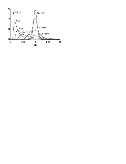
FIG. 1.: Distribution functions ${\cal P}^{(N)}_{u}(x;\{\kappa\})$ of the absorption coefficient in the unit of its average value for $N$-uncoupled dots. Plottings are shown for (a) $\gamma=0.1$ and (b) $\gamma=10$, where $\gamma=\pi\Gamma/\Delta$ and $\Gamma$ and $\Delta$ are the level width and the mean level spacing.

REFERENCES

• [1] B. L. Altshuler, P. A. Lee, and R. A. Webb, Mesoscopic Phenomena in Solids, (North-Holland, Amsterdam, 1991).
• [2] R. W. Siegel, Physics Today, 46, 64 (1993).
• [3] A. I. Ekimov and Al. L. Efros, Phys. Status Solidi B 150, 627 (1988).
• [4] Al. L. Efros in Phonons in Semiconductor Nanostructures, eds. J.-P. Leburton, J. Pascual, C. Sotomayor Torres, (KAP. Boston, London, NATO AS-v.236, 1993).
• [5] M. L. Mehta, Random Matrices, 2nd ed. (Academic Press, San Diego, CA, 1991); F. Haake, Quantum Signatures of Chaos (Springer-Verlag, Berlin, 1991).
• [6] V. N. Prigodin et. al., Phys. Rev. Lett. 75, 2392 (1995), 76, 1982 (1996); V. N. Prigodin and N. Taniguchi (to be published in Mod. Phys. Lett.).
• [7] Y. Alhassid and C. H. Lewenkopf, Phys. Rev. Lett. 75, 3922 (1995); M. Srednicki (unpublished, cond-mat).
• [8] B. L. Altshuler and B. D. Simons, in Mesoscopic Quantum Physics, eds. by E. Akkermans, G. Montambaux, J.-L. Pichard, and J. Zinn-Justin (North-Holland, Amsterdam, in press).
• [9] N. Dupuis and G. Montambaux, Phys. Rev. B 43, 14390 (1991).
• [10] H. Friedrich and D. Wintgen, Phys. Rep. 183, 37 (1989).
• [11] N. Taniguchi, A. V. Andreev, and B. L. Altshuler, Europhys. Lett. 29, 515 (1995).
• [12] C. E. Porter, Statistical Theory of Spectra: Fluctuations, (Academic Press, New York, 1965).
• [13] K. B. Efetov and V. N. Prigodin, Phys.Rev.Lett. 70, 1315 (1993); C. W. Beenakker, Phys.Rev. B 50, 15170 (1994).
• [14] K. B. Efetov, Adv. Phys. 32, 53 (1983). See also J. J. M. Verbaarschot, H. A. Weidenmüller and M. R. Zirnbauer, Phys. Rep. 129, 367 (1985).
Refer to caption
Refer to caption