1 Introduction

The physics of flexible membranes, two-dimensional surfaces fluctuating in three dimensions, is extremely rich, both on the theoretical side, where there is a nice interplay between geometry, statistical mechanics and field theory, and on the experimental side, where model systems abound.

The simplest examples of 2-dimensional surfaces are monolayers, or films—these are strictly planar systems. The statistical behaviour of monolayers falls into three distinct universality classes, depending on the microscopic interactions of the system. There are crystalline monolayers, with quasi-long-range translational order and long-range orientational order, hexatic monolayers, with short-range translational order but quasi-long-range orientational order, and fluid monolayers, with short-range translational and orientational order [1].

Physical membranes, 2-dimensional surfaces fluctuating in a 3-dimensional embedding space, are expected to have an equally rich phase structure. The simplest class of membranes is the crystalline class, in which topological defects, dislocations, and disclinations, are forbidden. At the discrete level crystalline membranes may be modelled by triangulated surfaces with fixed local connectivity. In this paper we will be concerned with the properties of a particularly simple model of a phantom (non self-avoiding) crystalline membrane, with emphasis on a critical analysis of the existence and stability of an ordered flat phase of the model for sufficiently large bending rigidity.

Crystalline membranes, also known as tethered or polymerised membranes, are the natural generalisation of linear polymer chains to two dimensions. Polymer chains in a good solvent crumple into a fractal object with Hausdorff dimension 5/3 (Flory exponent $\nu=3/5$). Crystalline membranes with in-plane solid-like elasticity, on the other hand, are predicted to exhibit quite different physical properties from their linear counterparts. In particular, they are expected to have a remarkable low-temperature ordered phase. This ordered, or flat, phase is characterised by long-range order in the orientation of surface normals. At high temperature, or equivalently low bending rigidity, phantom crystalline membranes will entropically disorder and crumple. Separating these two phases should be a crumpling transition, whose precise nature for physical membranes is still not fully understood.

Inorganic examples of crystalline membranes are thin sheets ($\leq 100$ Å) of graphite oxide (GO) in an aqueous suspension [2, 3] and the rag-like structures found in MoS₂ [4].

There are also beautiful biological examples of crystalline membranes such as the spectrin skeleton of red blood cell membranes. This is a two-dimensional triangulated network of roughly 70,000 plaquettes. Actin oligomers form nodes and spectrin tetramers form links [5]. Crystalline membranes can also be synthetised in the laboratory by polymerising amphiphillic monolayers or bilayers. For recent reviews see [6, 7, 8].

The existence of an ordered phase in a two dimensional system is remarkable, given the Mermin-Wagner theorem. In fact, if one thinks of surface normals as spins, then the membrane bending energy is akin to a Heisenberg interaction, and the $2d$-Heisenberg model is well known to have no ordered phase. What stabilises the flat phase in a crystalline membrane? There are several appealing arguments for the existence of a stable ordered phase in crystalline membranes [9]. Out-of-plane fluctuations of the membrane are coupled to in-plane “phonon” degrees of freedom because of the non-vanishing elastic moduli (shear and compressional) of a polymerised membrane. Bending of the membrane is inevitably accompanied by an internal stretching of the membrane. Integrating out the phonon degrees of freedom one finds long-range interactions between Gaussian curvature fluctuations which stabilise a flat phase for sufficiently large bare bending rigidity[9]. Alternatively both the elastic constants and the bending rigidity pick up anomalous dimensions in the field theory sense. The bending rigidity receives a stiffening contribution at large distances via the phonon coupling. This competes with the usual softening of bending rigidity seen in fluid membranes, with the net result being an ultraviolet-stable fixed point—the crumpling transition. From the magnetic point of view membrane models are constrained spin systems, since the spins must be normal to the underlying surface, and the constraints are essential to the stability of the ordered phase.

This viewpoint is supported by self-consistent calculations for the renormalisation of the bending rigidity, by large-$d$ calculations, where $d$ is the dimension of the embedding space, and by $\epsilon$-expansion calculations, where $\epsilon=4-D$, with the internal dimension $D$ of the membrane being 2 for physical polymerised membranes.

The construction of a discrete formulation of a crystalline membrane is essential for numerical simulations, and revealing for comparison with spin systems. In the simplest discretised version the membrane is modelled by a regular triangular lattice with fixed connectivity, embedded in $d$-dimensional space. Typically the link-lengths of the lattice are allowed some limited fluctuations. This may be modelled by tethers between hard spheres or by introducing some confining pair potential with short-range repulsion between nodes (monomers). The bending energy is represented by a ferromagnetic-like interaction between the normals to nearest-neighbour “plaquettes” [8].

In the random surface literature, on the other hand, it is more common bto consider a simple Gaussian spring model of the pair potential with vanishing equilibrium spring length. In this case the minimum link-lengths are unconstrained. A priori this model seems to be rather different from those above; one may worry that it is pathological in some sense. In particular one may ask if this model can ever generate the effective elastic constants which are required to stabilize a flat phase at large bending rigidity. To illustrate this concern consider the infinite bending rigidity limit of the model. In this limit the system becomes planar — out-of-plane fluctuations are completety suppressed. Since the pair potential allows it, what prevents all nodes from collapsing on each other within the plane of the membrane itself? The answer can be seen by considering what happens if a node moves across a bond, or if two nodes are exchanged. In this case the normals to some triangular plaquettes will inevitably be inverted. This generates a prohibitive bending energy cost and is effectively forbidden. The model thus dynamically generates a hard-core repulsion, and may be thought of as having an effective equilibrium spring length. In Appendix A we show that small fluctuations about a finite microscopic equilibrium spring length $a$ yield elastic constants proportional to ${(a/\epsilon)}^{2}$, where $\epsilon$ is the intrinsic lattice spacing. For $\epsilon\simeq a$ these constants are finite. For the model we consider, with vanishing microscopic $a$ and finite $\epsilon$, the heuristic arguments above suggest one should replace $a$ by an effective equilibrium spring length.

Monte Carlo simulations have in fact established strong evidence for a continuous crumpling transition in the model with $a=0$. Most of the simulations, however, have focused on the crumpling transition itself. Not much effort has been made to establish rigorously the existence and the properties of the flat phase. In the rest of this paper we present evidence that there is indeed a stable flat phase in this remarkably simple model of a crystalline membrane. Furthermore we show that the requisite elastic constants are dynamically generated with the correct scaling behaviour.

The paper is organised as follows: in Section 2 we discuss the discrete model, the numerical simulations and the choice of the boundary conditions. In Section 3 we review the evidence for the crumpling transition. In Section 4 we discuss the Monge representation of a surface and the theoretical predictions for asymptotically flat elastic surfaces. We then discuss our numerical results for the roughness exponent, the phonon fluctuations and the normal-normal correlation function. In Appendix A we give a calculation of the elastic constants of a discrete soft-core Gaussian model. In Appendix B we discuss of the methods used to measure the geodesic distance for the correlation function and in Appendix C we describe the parallel algorithm used to simulate the lattices with largest size.

2 Model

Figure 1: a) The intrinsic connectivity structure of the mesh. b) The labelling scheme: $\sigma$, $\rho$, $\tau$, $\mu$ are the intrinsic coordinates while $a$, $b$ label the triangles.

To describe a discrete polymerised surface we arrange $N$ particles (monomers) in a regular triangulation of a 2–$D$ manifold (see Fig. 1a). The 2–$D$ surface is then embedded in a $d$–dimensional space where it is allowed to fluctuate in all directions. Each monomer is labelled by a set of intrinsic coordinates ${\bf\sigma}=(\sigma_{1},\sigma_{2})$, with respect to a set of orthogonal axes in the 2–$D$ manifold. The position in the $d$–dimensional embedding space is given by the vector ${\bf x}_{\sigma}$. We will treat the case $d=3$.

In general, the Hamiltonian which describes these models has two terms: a pair potential and a bending energy term,

$${\cal H}={\cal H}_{T}+{\cal H}_{B}.$$ (1)

A commonly studied pair potential in the literature [10] is the tethering potential with hard core repulsion, given by

$${\cal H}_{T}=\sum_{\langle{\bf\sigma}{\rm{\sigma^{\prime}}}\rangle}V(|{\bf x}_{\sigma}-{\bf x}_{\sigma^{\prime}}|),$$ (2)

with

$$V(R)=\left\{\begin{array}[]{cl}\infty&R<a\\ 0&a\leq R\leq b\\ \infty&R>b\end{array}\right.,\;R=|{\bf x}_{\sigma}-{\bf x}_{\sigma^{\prime}}|$$ (3)

where $R$ is the link length, $a$ is the hard-core radius and $b$ is the tethering length.

We consider, instead, a model where the tethering potential is replaced by a simple Gaussian spring potential. The bending energy is the usual ferromagnetic interaction between the normals to the faces of the membrane, namely

$${\cal H}=\sum_{\langle\sigma\sigma^{\prime}\rangle}\left|{\bf x}_{\sigma}-{\bf x}_{\sigma^{\prime}}\right|^{2}+\kappa\sum_{\langle ab\rangle}\left(1-{\bf n}_{a}\cdot{\bf n}_{b}\right).$$ (4)

Here $\kappa$ is the bending rigidity, $a$ and $b$ label the faces of the surface and ${\bf n}_{a}$ is the unit normal to the face $a$. Both sums extend over nearest neighbours (see Fig. 1b). This action has no explicit short scale cut-off length or hard-core repulsion. Since there is no self-avoidance it represents a phantom surface. This action was investigated originally by Ambjørn et al. [11] and is inspired by the Polyakov action for Euclidean strings with extrinsic curvature [12, 13].

The main justification for studying phantom surfaces as models of realistic membranes is that in the flat phase self-avoidance is irrelevant [10, 14]. Although self-avoidance is expected to change the scaling behaviour at the critical point $\kappa_{c}$ and the nature of crumpled phase, it does not affect the scaling behaviour in the flat phase. As membranes with strong self-avoidance (and the resultant non-local interactions) are harder to simulate numerically, it is sensible to leave out self-avoidance when possible.

The partition function of this model is given by the trace of the Boltzmann weight over all possible configurations of the embedding variables ${\bf x}$:

$${\cal Z}=\int[d{\bf x}]~{}\delta({\bf x}_{cm})\;\exp(-{\cal H}[{\bf x}]).$$ (5)

Here ${\bf x}_{cm}$ is the centre of mass, which is held fixed to eliminate the translational zero mode. Expectation values are given by

$$\langle{\cal O}\rangle=\frac{1}{\cal Z}\int[d{\bf x}]~{}\delta({\bf x}_{cm}){\cal O}[{\bf x}]\exp(-{\cal H}[{\bf x}]).$$ (6)

We will consider the case of surfaces with the topology of the disk and free boundary conditions. Most experimental realisations of membranes have either this topology or spherical topology. Our choice also has certain technical advantages. To describe the flat phase we need to measure the finite-size-scaling of the thickness of the surface and the asymptotic behaviour of the normal-normal correlation function. With spherical or toroidal topology one would have to subtract the effects of the global shape of the surface.

2.1 Numerical Simulations

To evaluate the integral of Eq. (6) we use the Monte Carlo algorithm with a Metropolis update. In our case the Metropolis update corresponds to changing the position of a node by a trial vector $\vec{\epsilon}$ chosen randomly (and uniformly) in a box of size $(2\delta)^{3}$ centred on the old node position. The update is accepted if the change in the Hamiltonian is such that

$$\exp({\cal H}_{old}-{\cal H}_{new})>r,$$ (7)

where $r$ is a uniformly distributed random variable with values in the interval $[0,1)$. The value of $\delta$ is adjusted to keep the acceptance ratio around 50%. For a surface of linear size $L$, one Monte Carlo sweep corresponds to Metropolis update of all $L^{2}$ nodes. We used a lagged Fibonacci pseudo-random number generator.

$L$	$\kappa=1.1$	$\kappa=2.0$	$\tau_{R}\sim L^{z}$
32	$31\times 10^{6}$	$26\times 10^{6}$	$3\times 10^{4}$
46	$51\times 10^{6}$	$42\times 10^{6}$	$7\times 10^{4}$
64	$47\times 10^{6}$	$44\times 10^{6}$	$1.2\times 10^{5}$
128	$74\times 10^{6}$	—	$5\times 10^{5}$

Table 1: The number of thermalised sweeps collected per data point in the flat phase. The last column indicates the autocorrelation time for the slowest mode in the system, the radius of gyration. The autocorrelation time is comparable for both values of $\kappa$. The critical slowing down exponent $z\approx 2$, as expected for a local algorithm.

For the simulations we used both scalar and parallel machines: a MASPAR MP1 massively parallel processor, a 12-node IBM SP2 and an 8-node DEC Alpha farm. The SP2 and the Alphas were used as single independent CPUs, but we used a parallel Monte Carlo algorithm for the simulation of the largest lattice ($L=128$) on the MP1. We show in Table 1 the amount of thermalised data collected for the various lattice sizes and couplings in the flat phase. For the largest lattice we thermalised our surfaces by discarding about $10^{7}$ sweeps. In addition we have performed simulations close to the crumpling transition. This work is still in progress but preliminary results are discussed in Section 3.

Previous studies of the critical behaviour of crystalline surfaces used more elaborate simulation algorithms which combine a Langevin update with Fast Fourier Acceleration [15, 16, 17, 18, 19, 20, 21]. This algorithm is known to be more effective in reducing critical slowing down. We chose not to use this approach for several reasons. First of all it is very hard to implement the Fast Fourier Transform (FFT) on a 2-dimensional surface with free boundaries. Secondly the parallel computer we are using is less efficient on floating point intensive algorithms, such as Fourier Transforms. Finally, the Langevin algorithm suffers from systematic errors induced by the finite time step $\Delta t$. This necessitates an extrapolation to $\Delta t=0$, which can itself become time consuming.

Our statistical errors were estimated using two methods: the first is a direct measurement of the autocorrelation in the data and a corresponding correction of the standard deviation. The second is the standard jackknife algorithm. Both methods give consistent results.

2.2 Boundary Effects

The optimal shape for a triangulated surface with free boundaries is a hexagon. In our simulations the use of the parallel computer MP1 makes the hexagonal mesh inconvenient, since the layout of the CPUs is a square grid. When we map the regular triangulation to the square grid, the resulting surface has a rhomboidal shape, as can be seen from Fig. 2. In particular the regions in the shaded areas of Fig. 2 will be strongly influenced by the boundaries.

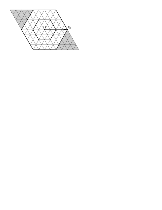
Figure 2: Two of the hexagons used to define the averages of the integrated observables. The arrow indicates the radius of the largest hexagon.

For a generic observable ${\cal O}_{\sigma}$ we want to be able to quantify the effect of the boundary and of the anisotropy. In order to achieve this we integrate the observable over hexagonal subsets of the mesh, centred with respect to the surface. Fig. 2 shows two of these subsets with darker lines. For a surface of linear size $L$ we construct $L/2$ such integrated observables by

$$\bar{\cal O}_{r}={1\over N_{r}}\sum_{\sigma\in H_{r}}{\cal O}_{\sigma}$$ (8)

where $H_{r}$ is a hexagon of radius $r$ and $N_{r}$ the appropriate normalisation. The shaded areas of Fig. 2 are discarded from the integration. By looking at larger and larger hexagons we can see when the boundaries start to affect the data. For very small hexagons the discretisation effects are large. In practice we find that the results are strongly influenced by the boundary for hexagons of radius $r>L/4$.

For non-integrated observables, such as the normal-normal correlation function, translational invariance in the surface is broken by the presence of the free boundary. Thus we always consider the correlation function from the centre of the surface to all the other nodes. The effect of the boundary can then be seen clearly on the correlations at a distance of order $L/4$. This boundary data is discarded from the fits.

3 Crumpling Transition

Before examining the flat phase of the model of Eq. (4) we would like to review the existing evidence for a “crumpling” transition. In recent years the crumpling transition has been the focus of extensive numerical and analytical investigation. Within the condensed-matter community it is customary to work with models with effective potentials like Eq. (2) and free boundaries [22, 10, 23]. Numerical simulations of these models provide direct evidence for a phase transition, such as a diverging specific heat, although the accuracy is not yet sufficient for a reliable determination of the specific heat exponent $\alpha$. When strong self-avoidance is included in the models described by Eq. (2), there is numerical evidence that the crumpling transition disappears altogether, with the system being flat for all bending rigidities [24, 25, 26, 27, 28]. Some studies of flexible impenetrable plaquettes, however, do find a crumpled phase [29, 30, 31]. The Gaussian spring models have been studied numerically in [15, 16, 17, 18, 19, 20, 11, 21, 32] using periodic boundary conditions, with emphasis on the precise nature of the phase transition. A growing peak in the specific heat is observed and the best estimate of the related critical exponent is $\alpha=0.58(10)$ [21].

There is thus strong evidence that models of phantom polymerised membranes have a continuous phase transition. We are also currently investigating this transition, and in the rest of this section we discuss our preliminary results.

3.1 Specific Heat

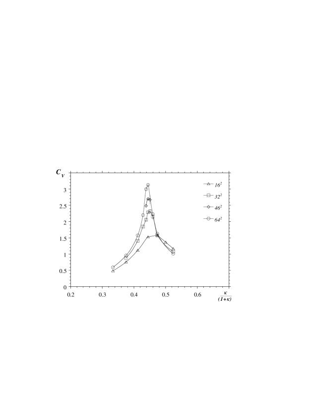
Figure 3: The specific heat versus bending rigidity.

Let us now turn to the energy fluctuations in our model. We write the total bending energy as

$$S_{e}=\sum_{\langle ab\rangle}{\bf n}_{a}\cdot{\bf n}_{b}.$$ (9)

Denoting the number of links (or edges) in the surface by $N_{e}$, it is simple to show [16] that the specific heat is given by

$$C_{V}=\frac{3(N-1)}{2}+\frac{\kappa^{2}}{N_{e}}(\langle S_{e}^{2}\rangle-\langle S_{e}\rangle^{2}).$$ (10)

Here the brackets indicate a statistical average over surfaces. We henceforth drop the constant piece from our analysis.

We plot in Fig. 3 the measured specific heat versus bending rigidity, for surfaces consisting of up to $64^{2}$ nodes. As expected we see a sharp peak at $\kappa\approx 0.79$ growing with system size. The critical behaviour of $C_{V}$ close to the phase transition is governed by an exponent $\alpha$, $C_{V}\sim|\kappa-\kappa_{c}|^{-\alpha}$, and for $\alpha<1$ the phase transition is continuous (as the first derivative of the free energy does not diverge). Hence it is important to determine the value of $\alpha$. The most convenient way of doing so is using finite size scaling, which predicts that the value of the peak should scale with volume as

$$C_{V}\;\approx\;c_{0}+c_{1}L^{\omega},$$ (11)

where, assuming hyperscaling, the specific heat exponent $\alpha={2\omega\over 2+\omega}$ and $c_{0}$ and $c_{1}$ are non-universal constants. Our best estimate of $\omega$, from the data shown in Fig. 3, is $\omega=0.5(1)$, consistent with previous results [21, 32]. The corresponding value of $\alpha$ is $0.4(1)$.

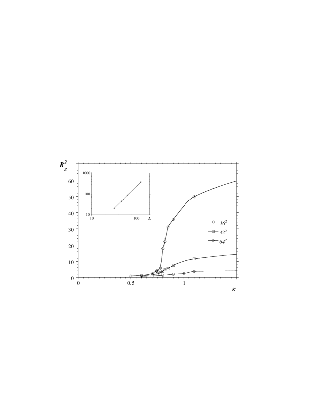
Figure 4: The radius of gyration as a function of $\kappa$ for various system sizes. In the inset we show a power-law fit for $R_{g}$ vs. $L$ at $\kappa=1.1$ for $L$ up to 128. We get $\nu=0.95(5)$.

3.2 Radius of Gyration

While the specific heat peak is one signal for the existence of a phase transition, it reveals little about the nature of the phases each side of the transition. An observable more sensitive to the geometry of the surface is the square of the radius of gyration,

$$R^{2}_{g}=\left\langle\frac{1}{3N}\sum_{\sigma}{\bf x}_{\sigma}\cdot{\bf x}_{\sigma}\right\rangle,$$ (12)

which measures the average spatial extent of the surface. $R_{g}$ defines a linear length scale for the surface and can be used to define a fractal or Hausdorff dimension $d_{H}$ in the embedding space via

$$R_{g}\sim N^{1/d_{H}}.$$ (13)

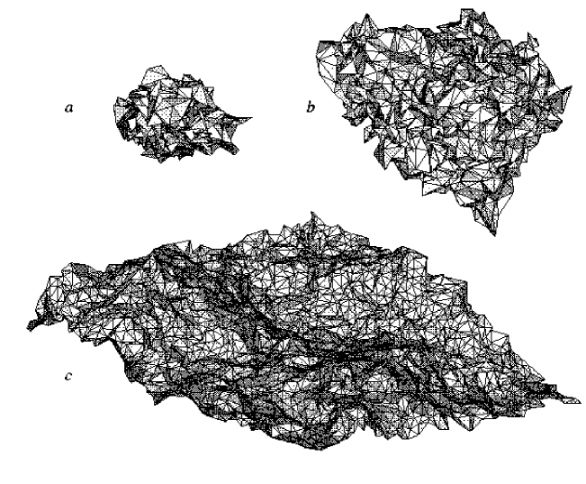
Figure 5: Snapshot of the surfaces with $L=46$ at (a) $\kappa=0.5$, (b) $\kappa=0.8$ and (c) $\kappa=2.0$. The average link length in each surface is comparable.

The Hausdorff dimension $d_{H}$ is related to the conventional Flory exponent $\nu$ ($R_{g}\sim L^{\nu}$) via $d_{H}=2/\nu$. For a flat surface, $\kappa>\kappa_{c}$, the radius of gyration scales linearly with the internal size, and hence $d_{H}=2$. In the high-temperature phase, on the other hand, $R_{g}$ scales logarithmically with the volume of the surface, $R_{g}\sim\log(N)$. In this case we say that the Hausdorff dimension is infinite ($\nu=0$). This justifies the terminology crumpled phase. This behavior can be computed exactly for $\kappa=0$ [11], while mean field theory or numerical methods are necessary for $\kappa<\kappa_{c}$ [15, 16, 17, 18, 19, 20, 21, 32]. Experimentally one can determine the Hausdorff dimension by measuring the structure function of diffracted light. A comparison with numerical simulations can be found in Ref. [33].

At the transition itself one might expect an intermediate behaviour (semi-crumpled surfaces) with $d_{H}>2$. Indeed this has been observed in [11], where it is claimed that $d_{H}=4$ at $\kappa_{c}$.

In Fig. 4 we show our measurements of the radius of gyration versus the bending rigidity for surfaces up to $64^{2}$ nodes. As expected, we see a dramatic change in their spatial extent as we pass through the phase transition. The surfaces literally blow up. This is better illustrated in Fig. 5, where we show snapshots of the surfaces: a in the crumpled phase, b at the phase transition and c in the flat phase.

We have only determined directly the Hausdorff dimension in the flat phase (for $\kappa=1.1$), where we have good statistics for surfaces up to $128^{2}$ nodes. The corresponding scaling plot is included in Fig. 4. A linear fit for surfaces larger than $16^{2}$ yields $d_{H}=2.1(1)$, or $\nu=0.95(5)$, as expected for a flat surface.

3.3 Normal-Normal Correlation Functions

As mentioned in Section 1, the different phases of a crystalline membrane can also be distinguished by the behaviour of the surface normals. In the flat phase the normals will have true long-range order, with the correlation function approaching a non-zero asymptote. In the crumpled phase the normals eventually decorrelate.

We define the normal-normal correlation function $G(r)$ as the scalar product of two normals on the surface separated by a distance of $r$ along the surface:

$$G(r)\;=\;\langle{\bf n}_{o}\cdot{\bf n}_{r}\rangle.$$ (14)

Here $o$ refers to the centre of the surface.

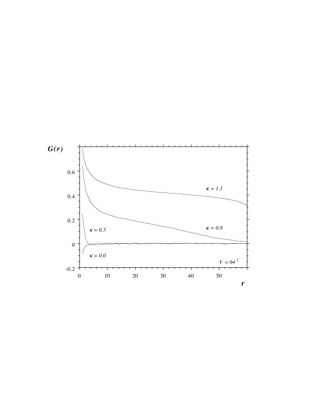
Figure 6: The correlation function $G(r)$ for various values of the bending rigidity $\kappa$.

In the crumpled phase we expect $G(r)$ to decay rapidly to zero. In fact in the exactly solvable $\kappa=0$ Gaussian model one finds that

$$G(r)=c_{1}{\delta(r)\over r^{2}}-{c_{2}\over r^{4}},$$ (15)

where $c_{1}$ and $c_{2}$ are cutoff-dependent constants and $\delta(r)$ is the two-dimensional regularised $\delta$-function [11]. In the discrete case, the normals become decorrelated over a few lattice steps.

We have measured $G(r)$ for several bending rigidities, both in the crumpled and flat phase. In Fig. 6 we illustrate this on lattices with $64^{2}$ nodes. For a more detailed discussion of how we perform the measurements we refer to Appendix B.

In the crumpled phase $G(r)$ decays very rapidly to zero and, for $\kappa=0$, we indeed see a negative correlation between the normals at short distances, as expected from Eq. (15). On a highly crumpled surface neighbouring triangles fold on each other. As $\kappa$ increases the normals become positively correlated at short distance, although $G(r)$ still becomes negative (for $\kappa<\kappa_{c}$) before decaying to zero.

At the critical point the normal-normal correlation function is expected to decay algebraically,

$$G(r)\sim{1\over r^{\bar{\eta}}},$$ (16)

with an exponent $\bar{\eta}$ different from the Gaussian value 4. This is consistent with our numerical results. A simple scaling argument [23] shows that $\bar{\eta}$ is related to the size (Flory) exponent $\nu$ by $\bar{\eta}=4(1-\nu)$. As we enter the critical region ($\kappa\approx 0.79$) the normal-normal correlation function still decays to zero, but now stays positive for all values of $r$. It is also clear that it decays to zero more slowly than in the crumpled phase. A crude estimate of the exponent $\bar{\eta}$, using a surface with $64^{2}$ nodes and $\kappa=0.79$, yields $\bar{\eta}\approx 0.71(5)$. This implies a size exponent $\nu=0.82(1)$ and hence Hausdorff dimension $d_{H}=2.4(2)$. This is consistent with previous numerical results [23] and maybe be compared with two theoretical predictions: $d_{H}=3$ from a $1/d$ renormalisation group calculation [34], applied to $d=3$, and $d_{H}=2.73$ from the self-consistent screening approximation [35].

Finally, we show in Fig. 6 a measurement of $G(r)$ for $\kappa=1.1$, i.e. in the flat phase. In that case we see a non-zero asymptote indicating true long-range-order in the normals. Fitting $G(r)$ to an algebraic decay plus a constant term excludes convincingly the possibility of a slow fall-off to zero, although eventually $G(r)$ becomes zero due to boundary effects. This behaviour is found consistently for surfaces of various sizes. We will return to the behaviour of the normal-normal correlation function in the flat phase in Section 4.4.

4 Flat Phase

Here we shall describe the current theoretical understanding of the flat phase of crystalline membranes. Given the Mermin-Wagner theorem it is important to understand what could stabilise an ordered phase in this two-dimensional system. This is most easily described in the Monge representation of a surface

$${\bf x}_{\sigma}=h_{\sigma}\hat{z}+{\bf r}_{\sigma},$$ (17)

where $h_{\sigma}$ is the height of the surface w.r.t. the base plane $\hat{x}-\hat{y}$ and ${\bf r_{\sigma}}$ is the projection of ${\bf x_{\sigma}}$ on the base plane. We define the phonon fluctuations ${\bf u}_{\sigma}$ of the surface by

$${\bf r}_{\sigma}={\bf s}_{\sigma}+{\bf u}_{\sigma}$$ (18)

where ${\bf s}_{\sigma}$ are the equilibrium positions of the nodes. An effective Hamiltonian for the flat phase [9, 36] is a sum of bending and elastic stretching energies

$${\cal H}(h,{\bf u})=\frac{\kappa}{2}\int d^{2}\sigma\,{(\nabla^{2}h)}^{2}+\frac{1}{2}\int d^{2}\sigma(2\mu\,u_{\alpha\beta}^{2}+\lambda\,u_{\gamma\gamma}^{2}),$$ (19)

where $\mu$ and $\lambda$ are the bare in-plane Lamé coefficients, $\kappa$ is the bending rigidity and $u_{\alpha\beta}$ is the strain tensor. This tensor measures the deformation of the induced metric from the flat metric, and is given by

$$u_{\alpha\beta} = {1\over 2}\left(\partial_{\alpha}{\bf x}\cdot\partial_{\beta}{\bf x}-\delta_{\alpha\beta}\right)$$ (20)

$$= \frac{1}{2}\{\nabla_{\alpha}u_{\beta}+\nabla_{\beta}u_{\alpha}+\nabla_{\negthinspace\alpha}h\nabla_{\negthinspace\beta}h\}.$$ (21)

to linear order in u. The indices $\alpha$, $\beta$ run over the internal coordinate $\sigma=(\sigma_{1},\sigma_{2})$.

One can integrate out the phonon degrees of freedom by performing the Gaussian integration[8]. One finds that the phonons give rise to an effective long-range two-point interaction for the scalar curvature. This interaction flattens the surface by stiffening the bending rigidity at large distances.

A more precise understanding may be obtained from self-consistent calculations of the renormalised bending rigidity [9, 35], mean-field calculations [37], the $\epsilon$-expansion ($\epsilon=4-D$, with $D$ the dimensionality of the surface) [38, 39] and the $1/d$ expansion (where $d$ is the embedding dimension) [34, 40]. Generally one finds that the renormalised bending rigidity is scale dependent with a non-vanishing anomalous dimension

$$\kappa_{R}(q)\sim q^{-\eta}.$$ (22)

At long wavelength $\kappa_{R}(q)$ is stiffened by short wavelength undulations of the membrane. It is also found that the elastic moduli $\mu$ and $\lambda$ are softened at long wavelength

$$\mu_{R}(q)\sim\lambda_{R}(q)\sim q^{\eta_{u}}.$$ (23)

The exponents $\eta$ and $\eta_{u}$ are not independent. Rotational invariance [38], or self consistent integral equations for the renormalised bending rigidity, imply

$$\eta=1-\frac{\eta_{u}}{2}.$$ (24)

An immediate implication of these anomalous dimensions or power-law singularities are non-trivial roughness exponents and height and in-plane displacement fluctuations or correlations. Defining a roughness exponent $\zeta$ by the finite-size-scaling of the mean-square height fluctuations in a box of size $L$

$$\langle h^{2}\rangle\;\sim\;L^{2\zeta},$$ (25)

we see from Eq. (19) that

$$\langle h^{2}\rangle\;\sim\;\int^{1\over a}_{1\over L}\frac{d^{2}q}{(2\pi)^{2}}\frac{1}{\kappa_{R}(q)\,q^{4}}\;\sim\;\int^{1\over a}_{1\over L}\frac{d^{2}q}{(2\pi)^{2}}\frac{1}{q^{4-\eta}}\;\sim\;L^{2-\eta},$$ (26)

implying $\zeta=1-\eta/2$. In the above $a$ is a short-distance regularisation cut-off. Similarly there is a non-trivial exponent for phonon fluctuations [41]

$$\langle|{\bf u}^{2}|\rangle\;\sim\;L^{\eta_{u}}.$$ (27)

In the framework of the self-consistent screening approximation it is possible to obtain analytic predictions for these exponents [35]. By assuming the scaling relations of Eqs. (22) and  (23) one can sum the terms in the perturbative expansion which renormalise $\kappa_{R}(q)$ and solve for the exponent $\eta$. In subsequent sections we shall describe our numerical measurements of these exponents.

Finally, a measure of long-range order in the flat phase is provided by the normal-normal correlation function. In the Monge representation a normal to the surface at point $\sigma$ is given by:

$${\bf n}_{\sigma}=\frac{\left(-\partial_{\sigma_{1}}h,-\partial_{\sigma_{2}}h,\;1\right)}{\sqrt{1+|\nabla h|^{2}}},$$ (28)

where $\sigma_{1}$ and $\sigma_{2}$ are the components of the intrinsic coordinate $\sigma$. To compute $\langle{\bf n}_{\sigma}\cdot{\bf n}_{o}\rangle$ we rotate the surface so that the normal at the origin coincides with the $\hat{z}$ axis. Hence

$${\bf n}_{\sigma}\cdot\left(0,\,0,\,1\right)\;=\;\frac{1}{\sqrt{1+|\nabla h_{\sigma}|^{2}}}\;\approx\;1-\frac{1}{2}|\nabla h_{\sigma}|^{2}.$$ (29)

The correlation function then follows from the height-field propagator,

$$\langle{\bf n}_{\sigma}\cdot{\bf n}_{o}\rangle\;\simeq\;1\;-\;\frac{1}{2}\int_{1\over r}^{1\over a}\frac{{\rm d}^{2}q}{(2\pi)^{2}}\;\frac{q^{2}}{\kappa_{R}(q)\;q^{4}}\;\approx\;C+\frac{c}{r^{\eta}}\,,$$ (30)

where $r$ is the geodesic distance between the point at $\sigma$ and the origin $o$ in the embedding space. Thus a power-law decay of the normal-normal correlation function to a non-zero asymptote provides a direct measure of the bending rigidity anomalous exponent $\eta$.

4.1 Shape Tensor

Figure 7: The distribution of eigenvalues $\rho(\lambda)$ of the inertia tensor. The number of nodes is $46^{2}$ and the hexagon radius is 17.

We now return to our numerical results. Detailed information about the shape of the surface in the embedding space is provided by examining averages of the eigenvalues of the inertia tensor. More precisely we study the shape tensor, defined as the anisotropic part of the inertia tensor:

$$I_{ij}[{\bf x}]=\frac{1}{3N}\sum_{\bf\sigma}x_{i}({\bf\sigma})x_{j}({\bf\sigma}),$$ (31)

where $i$ and $j$ refer to the components of ${\bf x}$. The full inertia tensor has an additional isotropic contribution proportional to $\delta_{ij}$ — this scales like $R_{g}^{2}$. As the shape tensor $I_{ij}$ is strongly influenced by the boundary (in fact contributions from the boundary region dominate the sum Eq. (31)), we restrict our measurements to a hexagonal subset of the mesh, as described in Section 2.2. If we refer the surface to the body-fixed frame defined by the eigenvectors and its centre of mass, the eigenvalues of $I_{ij}$, $\lambda_{i}$, are nothing but the dispersion of the $i$-th component of ${\bf x}$, averaged over the surface

$$\lambda_{i}=\left\langle\frac{1}{3N_{r}}\sum_{\sigma\in H_{r}}x^{2}_{i}(\sigma)\right\rangle,$$ (32)

where $N_{r}$ is the number of nodes inside a hexagon of radius $r$.

We obtain the eigenvalues $\lambda_{i}$ by diagonalising $I_{ij}$. The distribution of these eigenvalues, $\rho(\lambda)$, is distinctly different in the two phases. In Fig. 7 we show three examples of this. In the crumpled phase (a) $\rho(\lambda)$ has a single peak, implying a three-fold degeneracy of the eigenvalues. This is a simple consequence of the isotropy of a crumpled surface in the embedding space. The position of the peak indicates the average extension of the surface, while its width is related to the fluctuations about that value. At the phase transition (b) there is still a single peak in $\rho(\lambda)$, but now accompanied by a significant tail extending to large eigenvalues. This is due to increasing fluctuations in the size of the surface in the critical region.

The behaviour is very different for a flat surface (c). We now see two well resolved peaks in $\rho(\lambda)$ indicating, as expected, a broken $O(3)$ symmetry. There is a single minimum eigenvalue, corresponding to the left peak, which can be identified with the average square thickness of the surface. But there are also two almost degenerate large eigenvalues, as can be established by measuring the area of the right hand peak. This is a result of the remnant $O(2)$ symmetry in the plane. If we did not restrict our measurements to a hexagonal subset of the mesh, we would actually see three peaks in $\rho(\lambda)$, due to the anisotropy of the boundary.

4.2 Roughness Exponent

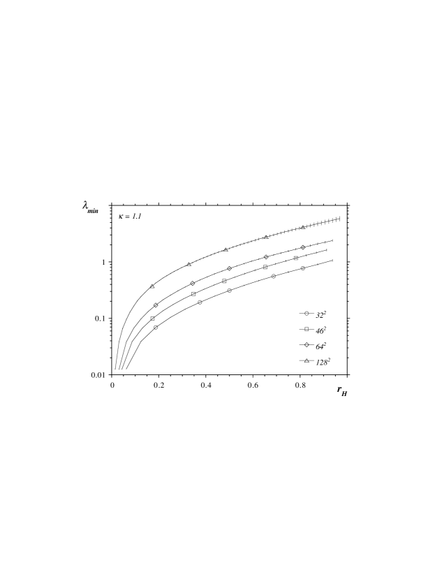
Figure 8: The minimum eigenvalue $\lambda_{min}$ versus the radius of the hexagon for various lattice sizes and $\kappa=1.1$. The solid lines are obtained from a polynomial fit and the points are simply to guide the eye.

To measure the height fluctuations in the flat phase, and the corresponding roughness exponent $\zeta$, we need an estimate of the out-of-plane fluctuations. This is provided by the minimum eigenvalue of the shape tensor which, as discussed in last section, is simply the average squared height. Hence

$$\lambda_{min}\;\sim\;\left\langle\int d^{2}{\sigma}\,h^{2}_{\sigma}\right\rangle\;\sim\;L^{2\zeta}.$$ (33)

In Fig. 8 we plot the minimum eigenvalue $\lambda_{min}$ versus the (normalised) radius of the hexagonal subsets we used, $r_{H}=2r/L$. This is shown for four different size surfaces at $\kappa=1.1$. A comment on how we treat the data: as we can only use hexagonal subsets of certain radii (discrete units of the lattice spacing), measurements on surfaces of different sizes will yield measurements at different values of the normalised radius $r_{H}$. To compare measurements from surfaces of different sizes, at the same value of $r_{H}$, we must therefore interpolate between the data points. These are the solid lines in Fig. 8. For the interpolation we used a polynomial fit, with the degree of the polynomials sufficiently large to yield a stable fit. We checked that different interpolation methods did not affect the results.

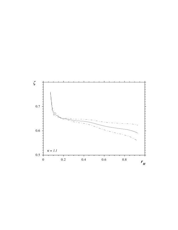
Figure 9: The roughness exponent $\zeta$ versus the normalised radius of the hexagon. We extract the value of $\zeta$ from the plateau region. The dashed lines indicate the size of the error bars. The bending rigidity is $\kappa=1.1$.

The roughness exponent $\zeta$ is then determined from the finite-size scaling of the minimum eigenvalue for a fixed value of $r_{H}$. The result is shown in Fig. 9. The solid line is $\zeta(r_{H})$ while the dashed lines indicate the error. There are large discretisation effects for small values of $r_{H}$, as expected. For $0.2\leq r_{H}\leq 0.5$ there is a reasonably stable value of the roughness exponent. Our best estimate from this intermediate region is $\zeta=0.64(2)$. This should be compared to the theoretical predictions $\zeta=.590$ [35] and $\zeta=2/3$ [34] and from measurements on the spectrin network $\zeta=0.65(10)$ [5]. Previous numerical investigations of models of tethered surfaces have found a wide range of values for $\zeta$. These include 0.5 [42], 0.53 [43], 0.56(2) [5], 0.6 [44], 0.64 [45, 26, 46], 0.65 [41, 47] and 0.70 [48, 31]. From the scaling relation $\eta=2(1-\zeta)$ we find $\eta=0.72(4)$. For larger values of $r_{H}$ we see clear evidence of boundary effects. Indeed, if we did not work with hexagonal subsets, we would not be able to extract a reliable estimate for $\zeta$.

We have also measured $\zeta(r_{H})$ for $\kappa=2.0$, although the largest surface simulated in this case had only $64^{2}$ nodes. Once again a finite-size-scaling analysis yields a stable value of $\zeta$ in the same interval of $r_{H}$. In this case the result is $\zeta=0.71(2)$. This value is 3$\sigma$ larger than the corresponding value at the same lattice size for $\kappa=1.1$. We believe that this is due to larger finite size effects and that our results are consistent with having universal critical exponents in the flat phase as predicted by the fixed point of Refs. [38, 49, 39, 50].

4.3 Phonon Fluctuations

Figure 10: The exponent $\eta_{u}$ as a function of the hexagon radius. The dashed lines indicate the size of the error bars.

We now examine the issue of the in-plane elastic degrees of freedom in the flat phase of our model. For convenience, we rotate the surface so that the eigenvector associated to the smallest eigenvalue points in the $\hat{z}$ direction. Projecting the surface onto the $\hat{x}{-}\hat{y}$ plane gives us a discretised analogue of the field ${\bf r}_{\sigma}$ of Eq. (17).

The first step in the analysis must be to determine the phonon field u_σ. We therefore need to determine the field ${\bf s}_{\sigma}$ giving the equilibrium positions of the nodes. As before, we restrict our analysis to the hexagonal subsets $H_{r}$ of Section 2.2. We assume that the equilibrium positions of the nodes lie exactly on a regular hexagon in the $\hat{x}{-}\hat{y}$ plane. In the course of the Monte Carlo simulation, the surface fluctuates in the embedding space so that the orientation of its principal axes and its overall extent change constantly. Thus we need to find the regular hexagon ${\bf s}_{\sigma}$ for each configuration we analyse. We define the functional

$$F\;=\;\sum_{\sigma}\left({\bf r}_{\sigma}-{\bf s}_{\sigma}\right)^{2}\;=\;\sum_{\sigma}{\bf u}_{\sigma}^{2},$$ (34)

and we choose the equilibrium position of the mesh to be best represented by the hexagon which minimises $F$. The regular hexagon s can be parametrised by the position of its centre, a rotation angle $\theta$ and a scale factor $\xi$. The centre of the hexagon is trivially set to coincide with the centre of mass of the projected surface. Minimizing the functional $F$ with respect to the angle $\theta$ and the scale $\xi$ yields a unique solution up to the six-fold symmetry of the regular hexagon $\theta\to\theta+\pi/6$. This six-fold degeneracy of the minimum of $F$ can be eliminated by requiring that the internal labels of the ${\bf s_{\sigma}}$ overlap with the ones of the ${\bf r}_{\sigma}$.

We determine the characteristic scaling exponent $\eta_{u}$, defined in Eq. 27, by a power law fit of $\langle{\bf u}^{2}\rangle_{r_{H}}$ to $L$, for fixed values of $r_{H}$. Fig. 10 shows the result of the fit for $\kappa=1.1$. We extract the value of the exponent from the plateau in the figure. This gives $\eta_{u}=0.50(1)$ at $\kappa=1.1$. The corresponding value of $\eta$ obtained from the scaling relation of Eq. (24) is $\eta=0.750(5)$. We also quote the results of the same analysis at $\kappa=2.0$: $\eta_{u}=0.40(1)$.

4.4 Correlations in the Flat Phase

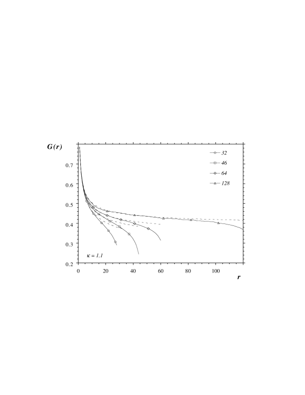
Figure 11: The $G(r)$ fall-off for $L=32$, $46$, $64$ and $128$. Representative data points are shown to guide the eye. The dashed lines are the best fits to Eq. (30).

In this section we treat the normal-normal correlation function in the flat phase. The measured correlation functions are shown in Fig. 11. We fit this correlation function to the expected power-law behaviour of Eq. (30)

$$G(r)=C+\frac{B}{r^{\eta}},$$ (35)

using a correlated least squares algorithm. We find a non-zero asymptote $C$ whose value tends to increase with lattice size. This is shown in Fig. 12.

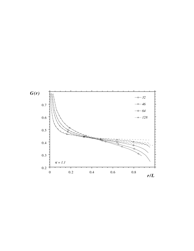
Figure 12: A plot of $G(r)$ with $r$ rescaled to show the finite-size effects on the asymptote ($\kappa=1.1$). This rescaling demonstrates that the asymptote stabilizes as the lattice size increases.

The correlated least squares algorithm attempts to minimise a chi-squared function of the form

$$\chi^{2}=\frac{1}{N(N-P)}\sum_{ij}^{N}(y_{i}-y^{*}_{i}(p_{i}))C_{ij}(y_{j}-y^{*}_{j}(p_{i})).$$ (36)

The data is fitted to a functional form $y^{*}_{i}(p_{i})$ where $i$ is the (lattice) geodesic distance and the quantities $\{p_{i}\},i=1\ldots P$, are the variational parameters in the fit. The matrix $C_{ij}$ is the inverse of the correlation matrix

$$C_{ij}=\left(M^{-1}\right)_{ij}$$ (37)

where

$$M_{rr^{\prime}}=\left\langle G\left(r\right)\,G\left(r^{\prime}\right)\right\rangle_{c}.$$ (38)

Note that for uncorrelated data the matrix $M$ is diagonal, and Eq. (36) reduces to the usual definiition of $\chi^{2}$. The inversion of this matrix is typically a delicate operation. Because of limited statistics it will often be close to singular and the smallest eigenvalues will only be poorly estimated from the data. In this situation it is necessary, and indeed correct, to restrict the inversion to an appropriate subspace that is spanned by eigenvectors with eigenvalues which are large enough to be estimated reliably from the data. This can be achieved through singular value decomposition techniques. The dimension of the subspace is referred to as the singular value decomposition (SVD) cut. For more details we refer the reader to [51].

In assessing the results of the fitting procedure we examined cases with a range of values of initial and final distances and SVD cuts. To obtain a $\chi^{2}$ of order unity we usually had to discard data from the last third of the path to the boundary and roughly one quarter of the eigenvalues.

	$\kappa$ = 1.1						$\kappa$ = 2.0
$L$	$C$		$\eta$		$\chi^{2}/$dof		$C$		$\eta$		$\chi^{2}/$dof
32	0.	181(16)	0.	331(7)	8.	6	0.	240(32)	0.	141(5)	14.	8
46	0.	274(9)	0.	397(5)	1.	66	0.	309(21)	0.	154(4)	2.	32
64	0.	321(5)	0.	447(6)	0.	96	0.	448(30)	0.	203(4)	2.	19
128	0.	383(6)	0.	521(6)	1.	14	—

Table 2: Fit to the correlation function $G(r)$.

	The constant $C$						The exponent $\eta$
$r_{min}$	$L=46$		$L=64$		$L=128$		$L=46$		$L=64$		$L=128$
1	0.	274(9)	0.	321(5)	0.	383(6)	0.	397(5)	0.	458(7)	0.	521(6)
2	0.	262(15)	0.	325(7)	0.	388(7)	0.	376(10)	0.	492(9)	0.	546(9)
3	0.	262(17)	0.	327(7)	0.	405(7)	0.	388(14)	0.	481(9)	0.	658(15)

Table 3: Effect of the short distance data ($\kappa=1.1$).

In Table 3 we show the fitted values of the asymptote $C$ and the exponent $\eta$. The fits are obtained including all the short distance data and we show only errors from the fit. It is clear that a more important source of error is finite size effects. Clearly both the constant $C$ and the exponent $\eta$ exhibit a shift with $L$ well in excess of the fitted errors. But this shift is systematic and indeed can be quantified by assuming a naive $1/L$ correction term to the correlation function $G(r)$. In that case the leading correction to $C$ will be $1/L$, while it is $\log(L)/L$ for the exponent $\eta$. This conjecture is in excellent agreement with our data, at least for $\kappa=1.1$, and implies infinite volume values of $C\approx 0.45$ and $\eta\approx 0.62$. This is in quantitative agreement with our previous estimates.

Another source of systematic error stems from discarding some of the short distance data. In Table 3 we show the results of fits to C and $\eta$ obtained by discarding data at distance $r<r_{min}$. It is clear that the values change with $r_{min}$, although not a great deal. Discarding short distance data increases the value of $\eta$ for the large lattices. This improves the comparison with the expected value.

Finally, a few comments on the data at $\kappa=2.0$. The values of $\eta$ quoted in Table 3 do not agree well with the values obtained at $\kappa=1.1$. But it should be mentioned that the fits to Eq. (35) are not as good in this case, which is reflected in higher values of the $\chi^{2}$.

5 Conclusions

In this paper we used a large scale Monte Carlo simulation to show that an extremely simple model of a crystalline membrane has a well-defined flat phase. In this phase the critical exponents are consistent both with previous simulations of tethered membranes and with theoretical predictions. In particular, the model we study has dynamically generated elastic moduli. The flat phase is convincingly demonstrated by the existence of a non-zero asymptote for the normal-normal correlation function, which strengthens with increasing system size. The flat phase exponents we find at $\kappa=1.1$ are: size (Flory) exponent $\nu=0.95(5)$ ($d_{H}=2.1(1)$), roughness exponent $\zeta=0.64(2)$, $\eta_{u}=0.50(1)$. A check on the consistency of our results for $\zeta$ and $\eta_{u}$ is obtained by comparing their respective scaling predictions for $\eta$. Our value of $\zeta$ implies $\eta\approx 0.72$ and our value of $\eta_{u}$ implies $\eta\approx 0.75$. These are consistent within our statistical errors. A direct measurement of $\eta$ from the power law decay of the normal-normal correlation functions is more difficult and is discussed in Section 4.4. For $L=128$ and $r_{min}=3$ we obtain $\eta=0.658(15)$. At higher bending rigidity we obtain somewhat different exponents, but we believe this is due to larger finite-size effects.

For completeness, we also establish that the model we consider has a crumpling transition. Preliminary determination of the critical exponents at the transition gives results consistent with existing simulations for related models.

Acknowledgments

David Nelson has contributed to this work with many suggestions and comments. We would also like to thank Mehran Kardar, Emmanuel Guitter, Alan Middleton, Paul Coddington and Gerard Jungman for helpful discussions. Enzo Marinari kindly provided the random-number generator routine used in our parallel code. We are grateful to NPAC (North-East Parallel Architecture Center) for the use of their computational facilities. The research of MB and MF was supported by the Department of Energy U.S.A. under contract No. DE-FG02-85ER40237. SC and GT were supported by research funds from Syracuse University. Part of the work of KA was done at the Institute for Fundamental Theory at Gainesville and was supported by DOE grant No. DE-FG05-86ER-40272. We also acknowledge the use of the software package Geomview for membrane visualisation and code development [52].

Appendix A: Elastic Constants in the Gaussian Model

As we noted in the introduction, there are several potential pathologies in a model in which the tethering potential contains no hard core repulsion, such as the one we treat in this paper. The effective elastic constants may vanish or be too weak to generate a stable flat phase. Even if the model possesses a flat phase it may belong to a different universality class from a model with bare elastic constants.

The simplest argument supporting such concerns arises from a mean field theory calculation of the elastic moduli of our discrete tethering potential along the lines of [53]. Consider an equilibrium spring length parameter $a$ in the pair potential of Eq. (4):

$${\cal H}_{T}(a) = \sum_{\langle\sigma\sigma^{\prime}\rangle}{\left(\left|{\bf x}_{\sigma}-{\bf x}_{\sigma^{\prime}}\right|-a\right)^{2}}$$ (39)

$$= {1\over 2}\sum_{\sigma}\sum_{\sigma^{\prime}}\left(\left|{\bf x}_{\bf\sigma}-{\bf x}_{\sigma^{\prime}}\right|-a\right)^{2}\,.$$ (40)

In the second sum $\sigma^{\prime}$ runs over the neighbour nodes of $\sigma$. Note that we have chosen units such that the spring constant $k/(k_{B}T)=1$ and x, u and ${\bf\sigma}$ are dimensionless. For $a$ sufficiently large we may describe the location of the nodes ${\bf x}_{\bf\sigma}$ by

$$\left({\bf x}_{\bf\sigma}-{\bf x}_{\rm{\sigma}^{\prime}}\right)_{\alpha}=\left(\delta_{\alpha\beta}+u_{\alpha\beta}\right){\bf s}_{\bf\sigma\sigma^{\prime}}^{\beta},$$ (41)

where ${\bf s}_{\bf\sigma}$ spans a regular hexagonal lattice, ${\bf s}_{\bf\sigma\sigma^{\prime}}={\bf s}_{\bf\sigma}-{\bf s}_{\bf\sigma^{\prime}}$ and $|{\bf s}_{\bf\sigma\sigma^{\prime}}|=a$. $\alpha$ and $\beta=1,2$ are intrinsic coordinate indices on the surface. Then

$$\left|{\bf x}_{\bf\sigma}-{\bf x}_{\rm{\sigma}^{\prime}}\right|^{2} = \left(\delta_{\alpha\beta}+2u_{\alpha\beta}+u_{\alpha\gamma}u_{\beta\gamma}\right){\bf s}_{\bf\sigma\sigma^{\prime}}^{\alpha}{\bf s}_{\bf\sigma\sigma^{\prime}}^{\beta}$$ (42)

$$= a^{2}+\left(2u_{\alpha\beta}+u_{\alpha\gamma}u_{\beta\gamma}\right){\bf s}_{\bf\sigma\sigma^{\prime}}^{\alpha}{\bf s}_{\bf\sigma\sigma^{\prime}}^{\beta}.$$ (43)

At this point we redefine $u^{\prime}_{\alpha\beta}=u_{\alpha\beta}+{1\over 2}u_{\alpha\gamma}u_{\beta\gamma}$ and subsequently drop the primes. This will not affect the end result to quadratic order. Expanding for small fluctuations $u_{\alpha\beta}\ll 1$ we have

$$\left|{\bf x}_{\bf\sigma}-{\bf x}_{\rm{\sigma}^{\prime}}\right| = \left(a^{2}+2u_{\alpha\beta}{\bf s}_{\bf\sigma\sigma^{\prime}}^{\alpha}{\bf s}_{\bf\sigma\sigma^{\prime}}^{\beta}\right)^{1\over 2}$$ (44)

$$\approx a+{1\over a}u_{\alpha\beta}{\bf s}_{\bf\sigma\sigma^{\prime}}^{\alpha}{\bf s}_{\bf\sigma\sigma^{\prime}}^{\beta}-{1\over 2a^{3}}u_{\alpha\beta}u_{\gamma\delta}{\bf s}_{\bf\sigma\sigma^{\prime}}^{\alpha}{\bf s}_{\bf\sigma\sigma^{\prime}}^{\beta}{\bf s}_{\bf\sigma\sigma^{\prime}}^{\gamma}{\bf s}_{\bf\sigma\sigma^{\prime}}^{\delta}+\ldots.$$ (45)

To evaluate Eq. (40), consider the 6 unit lattice vectors ${\bf d}_{b}$ of a regular hexagonal lattice where $b=1,\ldots,6$. Performing the sum over the neighbours ${\bf\sigma^{\prime}}$ gives

$${\cal H}_{T}(a) = {1\over 2}\sum_{\bf\sigma}\sum_{b=1}^{6}\left(au_{\alpha\beta}{\bf d}_{b}^{\alpha}{\bf d}_{b}^{\beta}\right)^{2}$$ (46)

$$= {3\over 8}a^{2}\sum_{\bf\sigma}\left(\delta^{\alpha\gamma}\delta^{\beta\delta}+\delta^{\alpha\delta}\delta^{\beta\gamma}+\delta^{\alpha\beta}\delta^{\gamma\delta}\right)u_{\alpha\beta}u_{\gamma\delta}$$ (47)

$$= {3\over 8}a^{2}\sum_{\bf\sigma}\left(2u_{\alpha\beta}u_{\beta\alpha}+u_{\gamma\gamma}^{2}\right).$$ (48)

For sufficiently large $N$, and $a$ fixed, one can approximate the above discrete sum with an integral.

$${\cal H}_{T}(a)\approx\int\frac{d^{2}\xi}{\epsilon^{2}}\left({\sqrt{3}\over 2}a^{2}u_{\alpha\beta}u_{\beta\alpha}+{\sqrt{3}\over 4}a^{2}u_{\gamma\gamma}^{2}\right),$$ (49)

where $\epsilon$ is the intrinsic lattice spacing. Often one is interested in the case $\epsilon\simeq a$. We keep the $\epsilon$ and $a$ dependence since we are interested in the case $a=0$, $\epsilon\neq 0$.

To determine the elastic constants recall that the most general continuum action for a crystalline membrane is [37]

$${\cal H} = \int d^{2}\xi\left[{\kappa\over 2}\partial^{2}{\bf x}\cdot\partial^{2}{\bf x}+u\left(\partial_{\alpha}{\bf x}\cdot\partial_{\beta}{\bf x}\right)^{2}\right.+$$ (50)

$$+\left.v\left(\partial_{\gamma}{\bf x}\cdot\partial_{\gamma}{\bf x}\right)^{2}+{t\over 2}\left(\partial_{\alpha}{\bf x}\cdot\partial_{\beta}{\bf x}\right)\right]$$

$$= \int d^{2}\xi\left[{\kappa\over 2}\partial^{2}{\bf x}\cdot\partial^{2}{\bf x}+\mu u_{\alpha\beta}u_{\beta\alpha}+{\lambda\over 2}u_{\gamma\gamma}^{2}+\tau u_{\gamma\gamma}\right],$$ (51)

where $u_{\alpha\beta}={1\over 2}(\partial_{\alpha}{\bf x}\cdot\partial_{\beta}{\bf x}-\delta_{\alpha\beta})$ is the strain tensor Eq. (20). The couplings in the two expressions in Eq. (50) are related by

$$u={\mu\over 4}\,,\qquad v={\lambda\over 8}\,,\qquad t=\tau-\mu-\lambda.$$ (52)

Thus the bare elastic constants, dimensionless in our units, arising from the lattice action (40) are

$$\mu=\lambda={\sqrt{3}\over 4}\frac{a^{2}}{\epsilon^{2}}\,,\qquad\tau=0.$$ (53)

Notice that if $\epsilon=a$ the elastic constants are independent of the lattice spacing. The model we have studied corresponds to the limit $a\rightarrow 0$ and $\epsilon$ fixed. In this limit fluctuations become large and the above calculation breaks down.

Appendix B: Measuring Correlation Functions

Figure 13: The comparison of the three methods used to measure the geodesic distance $r$. Methods A and B use the intrinsic metric. For method A we construct a piecewise linear path through the centre of each triangle, while for method B we construct a straight line between the centre of the starting and ending triangle. Method C is the same as A, except that it uses the induced metric to compute the distances between the triangles.

A necessary premise for measuring the normal-normal correlations function $G(r)$ is that we know the distance between two triangles on the surface. This distance can either be measured in the intrinsic metric (in which case it is trivial) or in the induced metric. For comparison we tested both methods.

Let us first describe our algorithm for determining distances in the induced metric at the discrete level. Given two points on the surface, we must find the shortest path, in the induced metric, along the surface. The problem here is that there are many definitions of “geodesic” which are equivalent in the continuum limit but differ at the discrete level. The algorithm we use is the following: given a triangle $t_{0}$ we find the distance from its centre to the centre of all its neighbours. Then we find the distance from those triangles to their neighbours (excluding triangles already visited). Iterating this procedure we find the minimum distance to each triangle from $t_{0}$, subject to the constraint that we have to pass through the centre of each triangle traversed. This is a piecewise linear approximation to the shortest path, which should be good for sufficiently large paths.

Similarly, for the intrinsic metric, we can either define the distance in units of jumps from triangle to triangle or, given that the vertices have explicit $(\sigma_{1},\sigma_{2})$ coordinates in the intrinsic formulation, we can define the shortest distance between them as a straight line.

We have verified that these different definitions of distances give identical results for the normal-normal correlation function measured in the flat phase (modulo a trivial rescaling of the $r$-axis). This is illustrated in Fig. 13. The relevance of this result goes beyond a simple consistency check: the fact that the geodesics defined intrinsically and extrinsically coincide means also that intrinsic and the extrinsic metric overlap in the flat phase.

All of the normal-normal correlation functions presented in the paper are obtained using method A.

Appendix C: Parallel Monte Carlo Algorithm

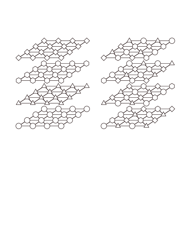
Figure 14: The improved parallelisation scheme. On the left we show the connectivity of the 4 different surfaces in the simulation, while on the right we show the actual internal representation. It is clear that, on the right, no node ever has a neighbour of the same type.

In this appendix we describe the parallel algorithm used on the MASPAR MP1. This machine is an old-style massively parallel computer with 16384 CPUs arranged in a $2-D$ ($128\times 128$) mesh with nearest neighbour connections. Each individual CPU is a relatively small processor (8 bit) with no floating-point unit.

A standard problem in using a parallel machine is the fact that the amount of parallelisation, and consequently the performance increase, is limited by the inter-dependence of the data. In order to ensure detailed balance in a Monte Carlo simulation, only a fraction of the lattice can be updated concurrently. In our case only 25% of the nodes can be updated. This translates into a huge performance loss as 75% of the nodes remain idle.

In order to overcome this limitation we implemented an improved parallelisation scheme. Instead of simulating one surface we consider 4 independent Monte Carlo simulations. The 4 corresponding meshes are “interleaved” in 4 arrays which store the node positions. Each surface is distributed onto the 4 arrays as shown in Fig. 14. The parallel machine updates one array at a time, but now each array holds independent data and therefore all of it can be updated in parallel.

We have compared the performance of this algorithm to the traditional parallelisation and to the sequential code. On the MASPAR, the traditional parallelisation, i.e. a Monte Carlo simulation of a single surface, can achieve a maximum speed of 80 Mflops (millions of floating-point operations per second). Our improved code is capable of 280 Mflops, almost a four-fold increase. This number is to be compared with the peak performance of this machine which, measured with the Linpack method, is around 440 Mflops. Our scalar code on an IBM RS/6000 390 with a clock of 66.5 MHz has a speed of 17 Mflops, compared to a Linpack peak performance of 54 Mflops.

The parallel algorithm also requires a careful implementation of the pseudo-random number generator. While the intrinsic MASPAR random number generator is known not to be reliable, using a sequential random number generator would be incredibly time consuming. The solution to this problem is to have an independent random number generator on each CPU, e.g. to regard it as an array-valued function. In order to avoid cross correlations between the random sequences generated by the parallel routine, a second standard random number routine is used to seed the array.

References

- [1] D. R. Nelson, in Fluctuating Geometries in Statistical Mechanics and Field Theory, edited by P. Ginsparg, F. David, and J. Zinn-Justin (cond-mat/9502114 or http://xxx.lanl.gov/lh94/, Les Houches, France, 1994), lectures given at the Les Houches Summer School.
- [2] X. Wen et al., Nature 355, 426 (1992).
- [3] T. Hwa, E. Kokufuta, and T. Tanaka, Phys. Rev. A 44, R2235 (1991).
- [4] R. R. Chianelli, E. B. Prestridge, T. Pecoraro, and J. P. DeNeufville, Science 203, 1105 (1979).
- [5] C. F. Schmidt et al., Science 259, 952 (1993).
- [6] L. Peliti, in Fluctuating Geometries in Statistical Mechanics and Field Theory, edited by P. Ginsparg, F. David, and J. Zinn-Justin (cond-mat/9501076 or http://xxx.lanl.gov/lh94/, Les Houches, France, 1994), lectures given at the Les Houches Summer School.
- [7] F. David, in Two Dimensional Quantum Gravity and Random Surfaces, Vol. 8 of Jerusalem Winter School for Theoretical Physics, edited by D. Gross, T. Piran, and S. Weinberg (World Scientific, Singapore, 1992).
- [8] Statistical Mechanics of Membranes and Surfaces, Vol. 5 of Jerusalem Winter School for Theoretical Physics, edited by D. Nelson, T. Piran, and S. Weinberg (World Scientific, Singapore, 1989).
- [9] D. Nelson and L. Peliti, J. Phys. France 48, 1085 (1987).
- [10] Y. Kantor and D. Nelson, Phys. Rev. Lett. 58, 2774 (1987).
- [11] J. Ambjørn, B. Durhuus, and T. Jonsson, Nucl. Phys. B 316, 526 (1989).
- [12] H. Kleinert, Phys. Lett. B 174, 335 (1986).
- [13] A. Polyakov, Nucl. Phys. B 268, 406 (1986).
- [14] Y. Kantor and K. Kremer, Phys. Rev. E 48, 2490 (1993).
- [15] M. Baig, D. Espriu, and J. Wheater, Nucl. Phys. B 314, 587 (1989).
- [16] R. Harnish and J. Wheater, Nucl. Phys. B 350, 861 (1991).
- [17] J. Wheater and T. Stephenson, Phys. Lett. B 302, 447 (1993).
- [18] M. Baig, D. Espriu, and A. Travesset, Nucl. Phys. B 426, 575 (1994).
- [19] D. Espriu and A. Travesset, Phys. Lett. B 356, 329 (1995).
- [20] D. Espriu and A. Travesset, 1996, hep-lat/9601005.
- [21] J. Wheater, Nucl. Phys. B 458, 671 (1996).
- [22] Y. Kantor, M. Kardar, and D. Nelson, Phys. Rev. Lett. 57, 791 (1986).
- [23] Y. Kantor and D. Nelson, Phys. Rev. A 36, 4020 (1987).
- [24] M. Plischke and D. Boal, Phys. Rev. A 38, 4943 (1988).
- [25] D. Boal, E. Levinson, D. Liu, and M. Plischke, Phys. Rev. A 40, 3292 (1989).
- [26] F. Abraham, W. Rudge, and M. Plischke, Phys. Rev. Lett. 62, 1757 (1989).
- [27] J. Ho and A. Baumgärtner, Phys. Rev. Lett. 63, 1324 (1989).
- [28] G. Grest and M. Murat, J. Phys. France 51, 1415 (1990).
- [29] A. Baumgärtner, J. Phys. I France 1, 1549 (1991).
- [30] A. Baumgärtner and W. Renz, Europhys. Lett. 17, 381 (1992).
- [31] D. Kroll and G. Gompper, J. Phys. France 3, 1131 (1993).
- [32] R. Renken and J. Kogut, Nucl. Phys. B 342, 753 (1990).
- [33] F. Abraham and M. Girardet, Europhys. Lett. 14, 293 (1992).
- [34] F. David and E. Guitter, Europhys. Lett. 5 (8), 709 (1988).
- [35] P. Le Doussal and L. Radzihovsky, Phys. Rev. Lett 69, 1209 (1992).
- [36] F. Abraham and D. Nelson, Science 249, 393 (1990).
- [37] M. Paczuski, M. Kardar, and D. Nelson, Phys. Rev. Lett. 60, 2639 (1988).
- [38] J. Aronovitz and T. Lubensky, Phys. Rev. Lett. 60, 2634 (1988).
- [39] E. Guitter, F. David, S. Leibler, and L. Peliti, Phys. Rev. Lett. 61, 2949 (1988).
- [40] M. Paczuski and M. Kardar, Phys. Rev. A 39, 6086 (1989).
- [41] F. Abraham and D. Nelson, J. Phys. France 51, 2653 (1990).
- [42] R. Lipowsky and M. Girardet, Phys. Rev. Lett. 65, 2893 (1990).
- [43] F. Abraham, Phys. Rev. Lett 67, 1669 (1991).
- [44] Z. Zhang, H. T. Davis, and D. M. Kroll, Phys. Rev. E 48, R651 (1993).
- [45] F. Abraham and D. Nelson, Science 249, 393 (1990).
- [46] S. Leibler and A. Maggs, Phys. Rev. Lett. 63, 406 (1989).
- [47] F. F. Abraham and M. Kardar, Science 252, 419 (1991).
- [48] G. Gompper and D. M. Kroll, J. Phys. I France 2, 663 (1992).
- [49] J. Aronovitz, L. Golubovic, and T. Lubensky, J. Phys. France 50, 609 (1989).
- [50] E. Guitter, F. David, S. Leibler, and L. Peliti, J. Phys. France 50, 1787 (1989).
- [51] S. Catterall, F. Devlin, I. Drummond, and R. Horgan, Phys. Lett. B 321, 246 (1994).
- [52] M. Phillips, S. Levy, and T. Munzner, Geomview: An Interactive Geometry Viewer, 1993, computers and mathematics column.
- [53] H. S. Seung and D. R. Nelson, Phys. Rev. A 38, 1005 (1988).