Self-organized branching processes: Avalanche models with dissipation

Abstract

We explore in the mean-field approximation the robustness with respect to dissipation of self-organized criticality in sandpile models. To this end, we generalize a recently introduced self-organized branching process, and show that the model self-organizes not into a critical state but rather into a subcritical state: when dissipation is present, the dynamical fixed point does not coincide with the critical point. Thus the level of dissipation acts as a relevant parameter in the renormalization-group sense. We study the model numerically and compute analytically the critical exponents for the avalanche size and lifetime distributions and the scaling exponents for the corresponding cutoffs.

PACS numbers: 64.60.Lx, 05.40.+j, 05.70.Ln, 05.20.-y

I Introduction

Many driven systems in nature respond to external perturbations by a hierarchy of avalanche events. This type of behavior is observed in magnetic systems [5], flux lines in superconductors [6], fluid flow through porous media [7], microfracturing processes [8], earthquakes [9], and physiological phenomena [10]. In these systems the distribution of avalanche amplitudes $s$ decays as a power law, $D(s)\sim s^{-\tau}$, thus suggesting an analogy with critical phenomena. Self-organized criticality (SOC) was proposed [11] as a possible framework to describe those phenomena. Power-law scaling would emerge spontaneously due to the dynamics, without the fine tuning of external parameters such as the temperature. Various models have been proposed with the aim of capturing the essential features of avalanche dynamics and self-organization. In particular, sandpile models stimulated an intense experimental [12, 13], numerical [14, 15] and theoretical [16, 17, 18] activity.

As in the case of phase transitions, mean-field theory represents the simplest approach that gives a qualitative description of the system. Mean-field exponents for SOC models have been obtained in different ways [19, 20, 21, 22, 23, 24, 25], but it turns out that their values (e.g., $\tau=3/2$) are the same for all the models considered thus far. This fact can easily be understood since the spreading of an avalanche in mean-field theory is a branching process [26] because an avalanche can be described by a front of “non-interacting particles” that can either trigger subsequent activity or die out. The connection between branching processes and SOC has been investigated, and it has been proposed that the mean-field behavior of sandpile models can be described by a critical branching process [27, 28, 29, 30].

However, the nature of the self-organization was not addressed by the previous approaches. In fact the branching process is critical only for a given value of the branching probability, while in sandpile models there is no such tuning. Recently, we have introduced the “self-organized branching process” (SOBP) [31], a mean-field model that allows one to clarify the mechanism of self-organization in sandpile models. Moreover, the SOBP model can be exactly mapped onto a two-state sandpile model in the limit $d\to\infty$, where $d$ is the dimension of the system.

In experiments it can be difficult to determine whether the cutoff in the scaling is due to finite-size effects or due to the fact that the system is not at but rather only close to the critical point. In this respect, it is important to test the robustness of SOC behavior by understanding which perturbations destroy the critical properties of SOC model.

It has been shown numerically [32, 33, 34] that the breaking of the conservation of particle numbers leads to a characteristic size in the avalanche distributions. Here we generalize the SOBP in order to allow for dissipation and we show, in the mean-field approximation, how the system self-organizes in a sub-critical state. In other words, the degree of nonconservation is a relevant parameter in the renormalization group sense [18].

In section II we derive the SOBP from a dissipative sandpile model. In section III we study the approach to the critical state. The critical exponents are evaluated in section IV, and the results are verified numerically. Section V is devoted to conclusions.

II Model and mean-field theory

Sandpile models are cellular automata with an integer or continuous variable $z_{i}$ (energy) associated with each site $i$ of a $d-$dimensional lattice. At each time step the energy of a randomly chosen site is increased by some amount. When the energy on a site reaches a threshold $z_{c}$ the site becomes unstable and relaxes by transferring its energy to its neighbors according to the specific rules of the model. In this way, a single relaxation can trigger other relaxations, leading to the formation of an avalanche. The boundary conditions are chosen to be open, so avalanches that reach the boundaries release energy outside of the system. After a transient, the system reaches a steady state characterized by a balance between the input and the output of energy.

Let us now consider a particular sandpile model: the two-state model introduced by Manna [35]. Energy can take only two stable values $z_{i}=0$ (empty site) and $z_{i}=1$ (particle). When $z_{i}\geq 2$ the site relaxes, $z_{i}\to z_{i}-2$, and the energy of two randomly chosen neighbors is increased by one. This rule conserves the energy, in this case the number of particles, during an avalanche and leads to a stationary critical state.

Some degree of nonconservation can be introduced in the model by allowing for energy dissipation in a relaxation event. In a continuous energy model this can be done by transferring to the neighboring sites only a fraction $(1-\epsilon)$ of the energy lost by the relaxing site [32]. In a discrete energy model, such as the Manna two-state model, one can introduce as the probability $\epsilon$ that the two particles transferred by the relaxing site are annihilated [33]. For $\epsilon=0$ one recovers the original two-state model.

Numerical simulations [32, 33] show that the two ways of considering dissipation lead to the same effect: a characteristic length is introduced into the system and the criticality is lost. As a result, the avalanche size distribution decays not as a pure power law but rather as

$$D(s)\sim s^{-\tau}\,h_{s}(s/s_{c}).$$ (1)

Here $h_{s}(x)$ is a cutoff function and the cutoff size scales as

$$s_{c}\sim\epsilon^{-\varphi}.$$ (2)

The size $s$ is defined as the number of sites that relax in an avalanche. We define the avalanche lifetime $T$ as the number of steps comprising an avalanche. The corresponding distribution decays as

$$D(T)\sim T^{-y}\,h_{T}(T/T_{c}),$$ (3)

where $h_{T}(x)$ is another cutoff function and $T_{c}$ is a cutoff that scales as

$$T_{c}\sim\epsilon^{-\psi}.$$ (4)

The cutoff or “scaling” functions $h_{s}(x)$ and $h_{T}(x)$ fall off exponentially for $x\gg 1$.

To construct the mean-field theory, we consider the model as $d\to\infty$ i.e. for an infinite dimensional lattice. When a particle is added to an arbitrary site, the site will relax if a particle was already present, which occurs with probability $p=P(z=1)$, the probability that the site is occupied. If a relaxation occurs, the two particles are transferred with probability $1-\epsilon$ to two of the infinitely many nearest neighbors, or they are dissipated with probability $\epsilon$.

Since $d\to\infty$ implies that the lattice coordination number tends to infinity, the avalanche will never visit the same site twice, implying that each site that receives a particle from a neighbor relaxes with the same probability. The avalanche process in the mean-field limit is a branching process. Moreover, we note that the branching process can be described by the effective branching probability

$$\tilde{p}\equiv p(1-\epsilon),$$ (5)

where $\tilde{p}$ is the probability to create two new active sites. From the theory of branching processes [26], we know that there is a critical value, $\tilde{p}=1/2$, or

$$p=p_{c}\equiv\frac{1}{2(1-\epsilon)},$$ (6)

such that for $p>p_{c}$ the probability to have an infinite avalanche is non-zero, while for $p<p_{c}$ all avalanches are finite. The value $p=p_{c}$ corresponds to the critical case where avalanches are power law distributed.

Boundary conditions are important for the process of self-organization. We can introduce the “boundary conditions” in the mean-field theory in a natural way by allowing for no more than $n$ generations for each avalanche. We can view the evolution of a single avalanche of size $s$ as taking place on a tree of $N=2^{n+1}-1$ sites (see Fig. 1). Note that we are not studying the model on a Bethe lattice [36]; i.e., the branching structure we are discussing is not directly related to the geometry of the system. The number of generations $n$ can, nevertheless, be thought of as some measure of the linear dimension of the system. If the avalanche reaches the boundary of the tree, we count the number of active sites $\sigma_{n}$ (which in the sandpile language corresponds to the energy leaving the system), and we expect that $p$ decreases for the next avalanche. If, on the other hand, the avalanche stops before reaching the boundary, then $p$ will slightly increase.

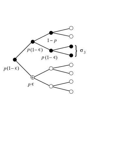
FIG. 1.: Schematic drawing of an avalanche in a system with a maximum of $n=3$ avalanche generations corresponding to $N=2^{n+1}-1=15$ sites. Each black site ($\bullet$) can relax in three different ways: (i) with probability $p(1-\epsilon)$ to two new black sites, (ii) with probability $1-p$ the avalanche stops, and (iii) with probability $p\epsilon$ two particles are dissipated at a black site, which then becomes a marked site ($\oplus$), and the avalanche stops. The black sites are part of an avalanche of size $s=6$, whereas the active sites at the boundary yield $\sigma_{3}(p,t)=2$. The total number of “stopped” sites are $\mu=2$, and there was one dissipation event such that $\kappa=2$.

To make the above statements quantitative, consider the evolution of the total number of particles $M(t)$ in the system after each avalanche:

$$M(t+1)=M(t)+1-\sigma(p,t)-\kappa(p,t).$$ (7)

Here $\sigma$ is the number of particles that leave the system from the boundaries and $\kappa$ is the number of particles lost by dissipation. Since $M(t)=NP(z=1)=Np$, we obtain an evolution equation for the parameter $p$:

$$p(t+1)=p(t)+\frac{1-\sigma(p,t)-\kappa(p,t)}{N}.$$ (8)

This equation reduces to the SOBP model [31] for the case of no dissipation ($\kappa=0$). The implications of Eq. (8) will be discussed in the following sections.

III Self-organization: the properties of the steady state

In order to characterize the steady state of the SOBP model, we rewrite Eq. (8) in terms of the average values of $\sigma$ and $\kappa$ indicated by angular brackets. The average number of particles $\left<\sigma_{n}\right>$ leaving the system from the boundaries in a system of $n$ generations is computed [26] because of the recursive nature of the process:

$$\left<\sigma_{n}(p,t)\right>=(2p(1-\epsilon))^{n}.$$ (9)

The evaluation of the average number of particles dissipated during an avalanche is somewhat more involved. We can first relate the average value of $\kappa$ to the average number of sites $\mu$ where an avalanche does not branch—either because of dissipation or because the site was empty (i.e., the avalanche stops),

$$\left<\kappa\right>=2\left<\mu\right>\frac{p\epsilon}{p\epsilon+1-p}.$$ (10)

The calculation of $\left<\kappa\right>$ then reduces to the calculation of $\left<\mu\right>$. If we denote by $\sigma_{m}$ the number of active sites at generation $m$, then $\mu$ is given by

$$\mu=\sum_{m=0}^{n-1}\left(\sigma_{m}-\frac{\sigma_{m+1}}{2}\right)=\frac{1+s-2\sigma_{n}}{2},$$ (11)

where $s=\sum_{m=0}^{n}\sigma_{m}$ is the total size of the avalanche. The average value of $s$ is obtained by summing the series:

$$\left<s\right>=\sum_{m=0}^{n}\left<\sigma_{m}\right>=\frac{1-(2p(1-\epsilon))^{n+1}}{1-2p(1-\epsilon)}.$$ (12)

Combing Eqs. (9)-(12), one obtains that Eq. (8) in the continuum notation becomes

  

$$\frac{dp}{dt}=\frac{1}{N}\left(1-(2p(1-\epsilon))^{n}-\frac{p\epsilon}{p\epsilon+1-p}\left[1+\frac{1-(2p(1-\epsilon))^{n+1}}{1-2p(1-\epsilon)}-2(2p(1-\epsilon))^{n}\right]\right)+\frac{\eta(p,t)}{N}.$$ (13)

  

In Eq. (13), we introduced the function $\eta(p,t)$ to describe the fluctuations around the average values of $\sigma$ and $\kappa$. We have shown numerically that the effect of this “noise” term is vanishingly small in the limit $N\to\infty$.

Without the noise term we can study the fixed points of Eq. (13). We find that there is only one fixed point,

$$p^{*}=1/2,$$ (14)

independent of the value of $\epsilon$; the corrections to this value are of the order $O(1/N)$. By linearizing Eq. (13), we find that the fixed point is attractive. This result implies that the SOBP model self-organizes into a state with $p=p^{*}$. In Fig. 2 we show the value of $p$ as a function of time for different values of the dissipation $\epsilon$. We find that independent of the initial conditions after a transient $p(t)$ reaches the self-organized steady-state described by the fixed point value $p^{*}=1/2$ and fluctuates around it with short-range correlations (of the order of one time unit). The fluctuations around the critical value decrease with the system size as $1/N$. Thus it follows that in the limit $N\to\infty$ the distribution $\phi(p)$ of $p$ approaches a delta function

$$\phi(p)\sim\delta(p-p^{*}).$$ (15)

By comparing the fixed point value (14) with the critical value (6), we obtain that in the presence of dissipation ($\epsilon>0$) the self-organized steady-state of the system is subcritical. Fig. 3 is a schematic picture of the phase space of the model, including the line $p=p_{c}$ of critical behavior (6) and the line $p=p^{*}$ of fixed points (14). These two lines intersect only for $\epsilon=0$.

FIG. 2.: The value of the control parameter $p(t)$ as a function of time for a system with different levels of dissipation. After a transient, $p(t)$ reaches its fixed-point value $p^{*}=1/2$ and fluctuates around it with short-range time correlations.

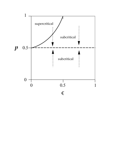
FIG. 3.: Phase diagram for the SOBP model with dissipation. The dashed line shows the fixed points $p^{*}=1/2$ of the dynamics, with the flow being indicated by the arrows. The solid line shows the critical points, cf. Eq. (6).

IV Critical exponents

In this section, we study the critical properties of the model. In the limit $n\gg 1$ we obtain analytical results for the avalanche and lifetime distributions for any value of $\tilde{p}$, the effective branching probability defined in Eq. (5). We show that the critical branching process with $\tilde{p}=1/2$ (obtained when $\epsilon=0$) correctly reduces to the mean-field exponents $\tau=3/2$ and $y=2$.

A Generating functions

The quantities $P_{n}(s,\tilde{p})$ and $Q_{n}(\sigma,\tilde{p})$ are defined to be the probabilities of an avalanche of size $s$ and boundary size $\sigma$ respectively, in a system with $n$ generations. The corresponding generating functions are defined by [26]

$$f_{n}(x,\tilde{p})\equiv\sum_{s}P_{n}(s,\tilde{p})x^{s},$$ (17)

$$g_{n}(x,\tilde{p})\equiv\sum_{\sigma}Q_{n}(\sigma,\tilde{p})x^{\sigma}.$$ (18)

From the hierarchical structure of the branching process, it is possible to write down recursion relations for $P_{n}(s,\tilde{p})$ and $Q_{n}(\sigma,\tilde{p})$, from which we obtain [26]

$$f_{n+1}(x,\tilde{p})=x\left[(1-\tilde{p})+\tilde{p}f^{2}_{n}(x,\tilde{p})\right]$$ (20)

and

$$g_{n+1}(x,\tilde{p})=(1-\tilde{p})+\tilde{p}g^{2}_{n}(x,\tilde{p}),$$ (21)

where $f_{0}(x,\tilde{p})=g_{0}(x,\tilde{p})=x$.

B Avalanche size distribution

The solution of Eq. (20) in the limit $n\gg 1$ is given by

$$f(x,\tilde{p})=\frac{1-\sqrt{1-4x^{2}\tilde{p}(1-\tilde{p})}\,}{2x\tilde{p}}.$$ (22)

We expand Eq. (22) as a series in $x$, and by comparing with the definition (17), we obtain for sizes such that $1\ll s\lesssim n$ [37]

$$P_{n}(s,\tilde{p})=\frac{\sqrt{2(1-\tilde{p})/\pi\tilde{p}}}{s^{3/2}}\,\exp\left(-s/s_{c}(\tilde{p})\right).$$ (23)

The cutoff $s_{c}(\tilde{p})$ is given by

$$s_{c}(\tilde{p})=-\frac{2}{\ln 4\tilde{p}(1-\tilde{p})}.$$ (24)

For avalanches with $n\lesssim s\lesssim N$ it is possible to use a Tauberian theorem [38, 39, 40], and show that $P_{n}(s,\tilde{p})$ will decay exponentially.

The next step is to calculate the avalanche distribution $D(s)$ for the SOBP model. This can be calculated as the average value of $P_{n}(s,\tilde{p})$ with respect to the probability density $\phi(p)$, i.e., according to

$$D(s)=\int_{0}^{1}dp\,\phi(p)\,P_{n}(s,\tilde{p}).$$ (25)

Since the simulation results show that $\phi(p)$ for $N\gg 1$ approaches the delta function $\delta(p-p^{*})$ [cf. Eq. (15)], expression (25) reduces to

$$D(s)=\left.P_{n}(s,\tilde{p})\right|_{\tilde{p}=p^{*}(1-\epsilon)}.$$ (26)

As a result we obtain the distribution

$$D(s)=\sqrt{\frac{2}{\pi}\,}\,\frac{1+\epsilon+\ldots}{s^{\tau}}\exp\left(-s/s_{c}(\epsilon)\right).$$ (27)

We can expand $s_{c}(\tilde{p})$ in $\epsilon$ with the result

$$s_{c}(\epsilon)\sim\frac{2}{\epsilon^{\varphi}},~{}~{}~{}~{}~{}~{}\varphi=2.$$ (28)

Furthermore, the mean-field exponent for the critical branching process is obtained setting $\epsilon=0$, i.e.,

$$\tau=3/2.$$ (29)

These results are in excellent agreement with the simulation of $D(s)$ for the SOBP model (cf. Fig. 4). The deviations from the power-law behavior (27) are due to the fact that Eq. (23) is only valid for $1\ll s\lesssim n$ [37].

FIG. 4.: (a) Log-log plot of the avalanche distribution $D(s)$ for different levels of dissipation. A line with slope $\tau=3/2$ is plotted for reference, and it describes the behavior of the data for intermediate $s$ values, cf. Eq. (27). For large $s$, the distributions fall off exponentially. (b) Data collapse produced by Eq. (27).

C Lifetime distribution

The avalanche lifetime distribution $D(T)$ is defined, for the model, as the probability to obtain an avalanche which spans $m$ generations; here, we identify $m$ with the time $T$. It follows that

$$P(m,\tilde{p})=Q_{m+1}(\sigma=0,\tilde{p})-Q_{m}(\sigma=0,\tilde{p}).$$ (30)

As for the avalanche distribution $D(s)$ we have that $D(T)=P(m=T,\tilde{p})$ evaluated for $\tilde{p}=p^{*}(1-\epsilon)$.

For $\tilde{p}=1/2$ we use the general result [26]

$$\frac{1}{1-Q_{m}(\sigma=0,\tilde{p})}=1+m\tilde{p}+O(\ln m),~{}~{}~{}~{}m\gg 1,$$ (31)

and obtain

$$P(T,\tilde{p})=\frac{\tilde{p}^{-1}}{T^{2}}\left(1+O(\ln T/T)+\ldots\right).$$ (32)

Note the strong correction to scaling to $D(T)$ in this case. For $\tilde{p}<1/2$ we find [26]

$$1-Q_{m}(\sigma=0,\tilde{p})\sim c_{1}(2\tilde{p})^{m},$$ (33)

FIG. 5.: (a) Log-log plot of the lifetime distribution $D(T)$ for different levels of dissipation. A line with slope $y=2$ is plotted for reference. Note the initial deviations from the power law for $\epsilon=0$ due to the strong corrections to scaling, cf. Eq. (32). (b) Data collapse produced by Eq. (34).

for $m\gg 1$, where $c_{1}>0$ is an unknown constant. This expression yields $D(T)\sim\epsilon\exp(-n\epsilon)$.

We can combine the above results in the scaling form

$$D(T)\sim T^{-y}\exp(-T/T_{c}),$$ (34)

where

$$T_{c}\sim\epsilon^{-\psi},~{}~{}~{}~{}~{}~{}\psi=1.$$ (35)

The lifetime exponent $y$ was defined in Eq. (3), wherefrom we obtain the mean-field result

$$y=2.$$ (36)

In Fig. 5, we show lifetime distributions for different values of $\epsilon$, together with the data collapse produced by Eq. (34).

V Discussion and conclusions

We have studied the effect of dissipation in the dynamics of the sandpile model in the mean-field limit ($d\to\infty$). In this limit, the dynamics of an avalanche is described by a branching process. We have derived an evolution equation for the branching probability that generalizes the self-organized branching process (SOBP) introduced in Ref. [31]. By analyzing this evolution equation, we have shown that there is a single attractive fixed point which in the presence of dissipation is not a critical point. The level of dissipation $\epsilon$ therefore acts as a relevant parameter for the SOBP model. We have determined analytically the critical exponents describing the scaling of the characteristic size with $\epsilon$ and the form of the avalanche distributions, and numerically verified the above results.

These results prove, in the mean-field limit, that criticality in the sandpile model is lost when dissipation is present. It would be interesting to use a similar approach for other forms of perturbations. In particular it has been shown for other SOC models that the presence of a non-zero temperature [41] or of a non-zero driving rate [42] are relevant perturbations leading to a non-critical steady state.

Finally, we discuss the relations between the SOBP model and the simplest possible SOC system recently introduced by Flyvbjerg [43]. The minimal definition of SOC, as a medium in which externally driven disturbances propagate leading to a stationary critical state, is well exemplified by the SOBP model. The disturbance is described by the branching process and the medium by the evolution equation for the density of particles in the system [Eq. (8)]. The example given by Flyvbjerg, being a two-state random-neighbor sandpile model, differs from the SOBP [31] in the way open boundary conditions are imposed.

REFERENCES

- [1]
- [2] Email: baekgard@nbi.dk
- [3] Email: zapperi@iris.bu.edu
- [4] Email: hes@buphy.bu.edu
- [5] P. J. Cote and L. V. Meisel, Phys. Rev. Lett. 67, 1334 (1991).
- [6] S. Field, J. Witt, F. Nori, and X. Ling, Phys. Rev. Lett. 74, 1206 (1995).
- [7] M. P. Lilly, P. T. Finley, and R. B. Hallock, Phys. Rev. Lett. 71, 4186 (1993); for a review see M. Sahimi, Rev. Mod. Phys. 65, 1393 (1993).
- [8] A. Petri, G. Paparo, A. Vespignani, A. Alippi, and M. Costantini, Phys. Rev. Lett. 73, 3423 (1994).
- [9] G. Gutenberg and C. F. Richter, Ann. Geophys. 9, 1 (1956).
- [10] B. Suki, A.-L. Barabasi, Z. Hantos, F. Petak, and H. E. Stanley, Nature 368, 615 (1994); A.-L. Barabasi, S. V. Buldyrev, B. Suki, and H. E. Stanley, Phys. Rev. Lett. 76, 2192 (1996).
- [11] P. Bak, C. Tang, and K. Wiesenfeld, Phys. Rev. Lett. 59, 381 (1987); Phys. Rev. A 38, 364 (1988). For a review see P. Bak and M. Creutz, in Fractals and Disordered Systems, vol. II, eds. A. Bunde and S. Havlin (Springer Verlag, Heidelberg, 1993).
- [12] H. M. Jaeger, C.-H Liu, S. R. Nagel, Phys. Rev. Lett. 59, 381 (1989).
- [13] V. Frette, K. Christensen, A. Malthe-Sørensen, J. Feder, T Jøssang, and P. Meakin, Nature 379, 49 (1996).
- [14] L. P. Kadanoff, S. R. Nagel, L. Wu, and S. Zhu, Phys. Rev. A 39, 6524 (1989).
- [15] P. Grassberger and S. S. Manna, J. Phys. France 51, 1077 (1990).
- [16] D. Dhar and R. Ramaswamy, Phys. Rev. Lett. 63, 1659 (1989); D. Dhar, Phys. Rev. Lett. 64, 1613 (1991); S. N. Majumdar and D. Dhar, Physica A 185, 129 (1992).
- [17] L. Pietronero, A. Vespignani, and S. Zapperi, Phys. Rev. Lett. 72, 1690 (1994).
- [18] A. Vespignani, S. Zapperi, and L. Pietronero, Phys. Rev. E 51, 1711 (1995).
- [19] C. Tang and P. Bak, J. Stat. Phys. 51, 797 (1988).
- [20] D. Dhar and S. N. Majumdar, J. Phys. A 23, 4333 (1990).
- [21] S. A. Janowsky and C. A. Laberge, J. Phys. A 26, L973 (1993).
- [22] H. Flyvbjerg, K. Sneppen, and P. Bak, Phys. Rev. Lett. 71, 4087 (1993); J. de Boer, B. Derrida, H. Flyvbjerg, A. D. Jackson, and T. Wettig, Ibid. 73, 906 (1994).
- [23] A. Stella, C. Tebaldi, and G. Caldarelli, Phys. Rev. E 52, 72 (1995).
- [24] M. Katori and H. Kobayashi, Physica A, xxxx (1996).
- [25] H.-M. Bröker and P. Grassberger, Europhys. Lett. 30, 319 (1995).
- [26] T. E. Harris, The Theory of Branching Processes (Dover, New York, 1989).
- [27] P. Alstrøm, Phys. Rev. A 38, 4905 (1988).
- [28] J. Theiler, Phys. Rev. E 47, 733 (1993).
- [29] K. Christensen and Z. Olami, Phys. Rev. E 48, 3361 (1993).
- [30] R. García-Pelayo, Phys. Rev. E 49, 4903 (1994).
- [31] S. Zapperi, K. B. Lauritsen, and H. E. Stanley, Phys. Rev. Lett. 75, 4071 (1995).
- [32] S. S. Manna, L. B. Kiss, and J. Kertész, J. Stat. Phys. 61, 923 (1990).
- [33] B. Tadić, U. Nowak, K. D. Usadel, R. Ramaswamy, and S. Padlewski, Phys. Rev. A 45, 8536 (1992).
- [34] B. Tadić and R. Ramaswamy, cond-mat/9602092.
- [35] S. S. Manna, J. Phys. A 24, L363 (1991).
- [36] Exact results for a dissipative abelian sandpile on the Bethe lattice are reported in M. Markošová, J. Phys. A 28, 6903 (1995).
- [37] For small we have the exact results , , , and so forth.
- [38] W. Feller, An Introduction to Probability Theory and its Applications, Vol. 2, 2nd ed. (John-Wiley, New York, 1971).
- [39] S. Asmussen and H. Hering, Branching Processes (Birkhäuser, Boston, 1983).
- [40] G. H. Weiss, Aspects and Applications of the Random Walk (North-Holland, Amsterdam, 1994).
- [41] M. Vergeles, Phys. Rev. Lett. 75, 1969 (1995).
- [42] V. Loreto, L. Pietronero, A. Vespignani, and S. Zapperi, Phys. Rev. Lett. 75, 465 (1995).
- [43] H. Flyvbjerg, Phys. Rev. Lett. 76, 940 (1996).