Entropy and Information in Neural Spike Trains

Abstract

The nervous system represents time dependent signals in sequences of discrete action potentials or spikes; all spikes are identical so that information is carried only in the spike arrival times. We show how to quantify this information, in bits, free from any assumptions about which features of the spike train or input signal are most important, and we apply this approach to the analysis of experiments on a motion sensitive neuron in the fly visual system. This neuron transmits information about the visual stimulus, at rates of up to 90 bits/s, within a factor of two of the physical limit set by the entropy of the spike train itself.

As you read this text, optical signals reaching your retina are encoded into sequences of identical pulses, termed action potentials or spikes, that propagate along the $\sim 10^{6}$ fibers of the optic nerve from eye to brain. This spike encoding appears almost universal, occurring in animals as diverse as worms and humans, and spanning all the sensory modalities [1]. The molecular mechanisms for the generation and propagation of action potentials are well understood [2], as are the mathematical reasons for the selection of stereotyped pulses by the dynamics of the nerve cell membrane [3]. Less well understood is the function of these spikes as a code [4]: How do the sequences of spikes represent the sensory world, and how much information is conveyed in this representation?

The temporal sequence of spikes provides a large capacity for transmitting information, as emphasized by MacKay and McCulloch 45 years ago [5]. One central question in studies of the nervous system is whether the brain takes advantage of this large capacity, or whether variations in spike timing represent noise which must be averaged away [4, 6]. In response to a long sample of time varying stimuli, the spike train of a single neuron varies, and we can quantify this variability by the entropy per unit time of the spike train, ${\cal S}(\Delta\tau)$ [7], which depends on the time resolution $\Delta\tau$ with which we record the spike arrival times. If we repeat the same time dependent stimulus, we see a similar, but not precisely identical, sequence of spikes (Fig. 1). This variability at fixed input can also be quantified by an entropy, which we call the conditional or noise entropy per unit time ${\cal N}(\Delta\tau)$. The information that the spike train provides about the stimulus is the difference between the total spike train entropy and this conditional entropy, $R_{\rm info}={\cal S}-{\cal N}$ [7]. Because the noise entropy is positive (semi)definite, the entropy rate sets the capacity for transmitting information, and we can define an efficiency $\epsilon(\Delta\tau)=R_{\rm info}(\Delta\tau)/{\cal S}(\Delta\tau)$ with which this capacity is used [8]. The question of whether spike timing is important is really the question of whether this efficiency is high at small $\Delta\tau$ [4].

For some neurons, we understand enough about what the spike train represents that direct “decoding” of the spike train is possible; the information extracted by these decoding methods can be more than half of the total spike train entropy with $\Delta\tau\sim 1$ ms [8]. The idea that sensory neurons provide a maximally efficient representation of the outside world has also been suggested as an optimization principle from which many features of these cells’ responses can be derived [9]. But, particularly in the central nervous system [6], assumptions about what is being encoded should be viewed with caution. The goal of this paper is, therefore, to give a completely model independent estimate of entropy and information in neural spike trains as they encode dynamic signals.

We begin by discretizing the spike train into time bins of size $\Delta\tau$, and examining segments of the spike train in windows of length $T$, so that each possible neural response is a “word” with $T/\Delta\tau$ symbols. Let us call the normalized count of the $i^{\rm th}$ word ${\tilde{p}}_{i}$, and then the “naive estimate” of the entropy is

$$S_{\rm naive}(T,\Delta\tau;{\rm size})=-\sum_{i}{\tilde{p}}_{i}\log_{2}{\tilde{p}}_{i},$$ (1)

where the notation reminds us that our estimate of the entropy depends on the ${\rm size}$ of the data set we use in accumulating the histogram. The true entropy is

$$S(T,\Delta\tau)=\lim_{{\rm size}\rightarrow\infty}S_{\rm naive}(T,\Delta\tau;{\rm size}),$$ (2)

and we are interested in the entropy rate

$${\cal S}(\Delta\tau)=\lim_{T\rightarrow\infty}{{S(T,\Delta\tau)}\over{T}}.$$ (3)

The difficutly is that, especially at large $T$, very large data sets are required to ensure convergence of $S_{\rm naive}$ to the true entropy $S$.

Imagine that we have a spike train with mean spike rate $\bar{r}\sim 40$ spikes/s and we sample with a time resolution $\Delta\tau=3$ ms. In a window of $T=100$ ms, the maximum entropy consistent with this mean rate [4, 5] is $S\sim 17.8\,{\rm bits}$, and we will see that the entropy of real spike trains is not far from this bound. But then there are roughly $2^{S}\sim 2\times 10^{5}$ words with significant $p_{i}$, and if our naive estimation procedure is going to work, we need to have at least one sample of each word. If our samples come from nonoverlapping 100 ms windows, then we need more than three hours of data, and one might think that we need much more data than this to insure that the probability of each word is estimated with reasonable accuracy. Such large quantities of data are generally inaccessible for experiments on real neurons.

Here we report that it is possible to make progress despite these pessimistic estimates. First, we examine explicitly the dependence of our entropy estimates on the size of the data set and find regular behaviors [10] that can be extrapolated to the infinite data limit. Second, we evaluate robust upper [7] and lower [11] bounds on the entropy which serve as a check on our extrapolation procedure. Third, we are interested in the extensive component of the entropy in large time windows, and we find that a clean approach to extensivity is visible before sampling problems set in. Finally, for the neuron studied—the motion sensitive neuron H1 in the fly’s visual system—where we can actually collect many hours of data.

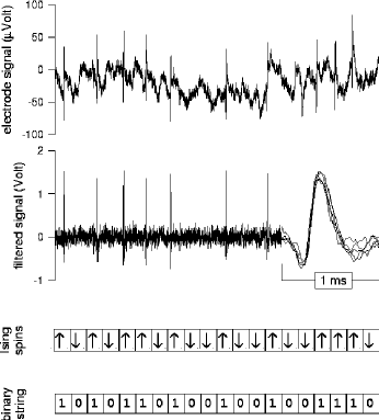
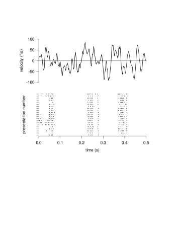
FIG. 1.: (A) Raw voltage records from a tungsten microelectrode near the cell H1 are filtered and discretized. (B) Angular velocity of a pattern moving across the fly’s visual field produces a sequence of spikes in H1, indicated by dots. Repeated presentations produce slightly different spike sequences. For experimental methods see Ref. [13].

H1 responds to motion across the entire visual field, producing more spikes for an inward horizontal motion and fewer spikes for an outward motion; vertical motions have no effect on this cell, but are coded by other neurons [12]. These cells provide visual feedback for flight control. In the experiments analyzed here [13], the fly is immobilized and views computer generated images on a display oscilloscope. For simplicity these images consist of a fixed pattern of vertical stripes with randomly chosen grey levels, and this pattern takes a random walk in the horizontal direction [14].

FIG. 2.: The frequency of occurence for different “words” in the spike train, with $\Delta\tau=3\,{\rm ms}$ and $T=30\,{\rm ms}$. Words are placed in order so that the histogram is monotonically decreasing; at this value of $T$ the most likely word corresponds to no spikes. Inset shows the dependence of the entropy, computed from this histogram according to Eq. (1) on the fraction of data included in the analysis. Also plotted is a least squares fit to the form $S=S_{0}+S_{1}/{\rm size}+S_{2}/{\rm size}^{2}$. The intercept $S_{0}$ is our extrapolation to the true value of the entropy with infinite data [10].

We begin our analysis with time bins of size $\Delta\tau=$ 3 ms. For a window of $T=30$ ms—corresponding to the behavioral response time of the fly [15]—we can estimate the entropy rather accurately by the naive procedure described above. Figure 2 shows the histogram $\{{\tilde{p}}_{i}\}$, and the naive entropy estimates. We see that there are very small finite data set corrections ($<10^{-3}$), well fit by [10]

$$S_{\rm naive}(T,\Delta\tau;{\rm size}) = S(T,\Delta\tau)+{S_{1}(T,\Delta\tau)\over{\rm size}}$$ (5)

$$\,\,\,\,\,+{{S_{2}(T,\Delta\tau)}\over{{\rm size}^{2}}}.$$

Under these conditions we feel confident that the extrapolated $S(T,\Delta\tau)$ is the correct entropy. For sufficiently large $T$, sampling problems occur: finite size corrections become much larger, the contribution of the second correction is significant and the extrapolation to infinite size is unreliable.

Ma [11] discussed the problem of entropy estimation in the undersampled limit. For probability distributions that are uniform on a set of $N$ bins (as in the microcanonical ensemble), the entropy is $\log_{2}N$ and the problem is to estimate $N$. Ma noted that this could be done by counting the number of times that two randomly chosen observations yield the same configuration, since the probability of such a coincidence is $1/N$. More generally, the probability of a coincidence is $P_{\rm c}=\sum p_{i}^{2}$, and hence

$$S = -\sum p_{i}\log_{2}p_{i}=-\langle\log_{2}p_{i}\rangle$$ (6)

$$\geq -\log_{2}\left(\langle p_{i}\rangle\right)=-\log_{2}P_{c},$$ (7)

so we can compute a lower bound the the entropy by counting coincidences. Furthermore, as emphasized by Ma, $\log_{2}P_{c}$ is less sensitive to sampling errors than is $S_{\rm naive}$. The Ma bound is the minimum entropy consistent with a given $P_{c}$, and it is one of the Renyi entropies [16]. It is also at the heart of algorithms for the analysis of attractors in dynamical systems [17].

The Ma bound is tightest for distributions that are close to uniform. The distributions of neural responses cannot be uniform because the spikes are sparse. But the distribution of words with fixed spike count, $N_{\rm sp}$, is more nearly uniform, so we apply the Ma bounding procedure in each $N_{\rm sp}$ sector. Thus $S\geq S_{\rm Ma}$, with

$$S_{\rm Ma} = -\sum_{N_{\rm sp}}P(N_{\rm sp})$$ (9)

$$\,\,\,\,\times\log_{2}\left[P(N_{\rm sp})\frac{2n_{c}(N_{\rm sp})}{N_{\rm obs}(N_{\rm sp})[N_{\rm obs}(N_{\rm sp})-1]}\right],$$

where $n_{c}(N_{\rm sp})$ is the number of coincidences observed among the words with $N_{\rm sp}$ spikes, $N_{\rm obs}(N_{\rm sp})$ is the total number of occurrences of words with $N_{\rm sp}$ spikes, and $P(N_{\rm sp})$ is the fraction of words with $N_{\rm sp}$ spikes.

In Fig. 3 we plot the entropy as a function of the window size $T$, with results both from the naive procedure and from the Ma bound. For sufficiently large windows the naive procedure gives an answer smaller than the Ma bound, and hence the naive answer must be unreliable because it is more sensitive to sampling problems. Before this sampling disaster the lower bound and the naive estimate are never more than 10–15% apart. The point at which the naive estimate crashes into the Ma bound is also where the second correction in Eq. (4) becomes significant and we lose control over the extrapolation to the infinite data limit. This occurs at $T\sim 100\ {\rm ms}$. We can trust the Ma bound beyond this point, but it becomes steadily less powerful.

FIG. 3.: The total and noise entropies per unit time (in bits per second) are plotted versus the reciprocal of the window size (in s^-1), with the time resolution held fixed at $\Delta\tau=3$ ms. Results are given both for the direct estimate and for the bounding procedure described in the text, and for each data point we apply the extrapolation procedures of Fig. 2 (inset). Dashed lines indicate extrapolations to infinite word length, as discussed in the text, and arrows indicate upper bounds obtained by differentiating $S(T)$ [7].

If the correlations in the spike train have finite range, then the leading subextensive contribution to the entropy will be a constant $C(\Delta\tau)$. This means that

$${{S(T,\Delta\tau)}\over{T}}={\cal S}(\Delta\tau)+{{C(\Delta\tau)}\over T}+\cdots.$$ (10)

This asymptotic behavior is seen clearly in Fig. 3, and emerges before the sampling disaster. Given the clean linear behavior in a well sampled region of the plot, we trust the extrapolation and arrive at an estimate of the entropy per unit time, ${\cal S}(\Delta\tau=3\,{\rm ms})=157\pm 3$ bits/s.

The entropy approaches its extensive limit from above [7], so that

$${1\over{\Delta\tau}}\left[S(T+\Delta\tau,\Delta\tau)-S(T,\Delta\tau)\right]\geq{\cal S}(\Delta\tau)$$ (11)

for all window sizes $T$. This bound becomes progressively tighter at larger $T$, until sampling problems set in. In fact there is a broad plateau ($\pm 2.7\%$) in the range $18<T<60$ ms, leading to $S\leq 157\pm 4$ bits/s, in excellent agreement with the extrapolation in Fig. 3.

The noise entropy per unit time ${\cal N}(\Delta\tau)$ measures the variability of the spike train when the input signals are held fixed. Hence we need to look at the ensemble of responses to repeated presentations of the same time varying input signal. Marking a particular time $t$ relative to the stimulus, we accumulate the frequencies of occurrence of each word $i$ that begins at $t$, and call this histogram $\tilde{p}_{i}(t)$. This generates a naive estimate of the local noise entropy in the window from $t$ to $t+T$,

$$N_{\rm naive}^{\rm local}(t,T,\Delta\tau;{\rm size})=-\sum_{i}\tilde{p}_{i}(t)\log_{2}\tilde{p}_{i}(t).$$ (12)

Estimating the average rate of information transmission by the spike train requires knowing the noise entropy averaged over $t$, $N_{\rm naive}(T,\Delta\tau;{\rm size})=\langle N_{\rm naive}^{\rm local}(t;T,\Delta\tau,{\rm size})\rangle_{t}$. Then we analyze as before the extrapolation to large data set ${\rm size}$ and large $T$. Fig. 3 also shows the noise entropy results as a function of the window size. The difference between the two entropies is the information which the cell transmits, $R_{\rm info}(\Delta\tau=3\,{\rm ms})=78\pm 5$ bits/s, or $1.8\pm 0.1$ bits/spike.

This anlysis has been carried out over a range of time resolutions, $800>\Delta\tau>2$ ms, and the results are summarized in Fig. 4. Over this range, the entropy per unit time of the spike train varies over a factor of roughly 40, illustrating the increasing capacity of the system to convey information by making use of spike timing. Note that $\Delta\tau=800$ ms corresponds to counting spikes in bins that contain typically thirty spikes, while $\Delta\tau=2$ ms corresponds to timing each spike to within 5% of the typical interspike interval. The information that the spike train conveys about the dynamics of motion across the visual field increases in approximate proportion to the entropy, corresponding to $\sim 50\%$ efficiency, at least for this ensemble of stimuli.

FIG. 4.: Information and entropy rates computed at various time resolutions, from $\Delta\tau=800\,{\rm ms}$ (lower left) to $\Delta\tau=2\,{\rm ms}$ (upper right). Note the approximately constant, high efficiency across the wide range of entropies.

Although we understand a good deal about the signals represented in H1 [12, 18], our present analysis does not hinge on this knowledge. Similarly, although it is possible to collect very large data sets from H1, Fig.’s 2 and 3 suggest that more limited data sets would compromise our conclusions only slightly. It is feasible, then, to apply these same analysis techniques to cells in the mammalian brain [19]. Like cells in the monkey or cat primary visual cortex, H1 is four layers ‘back’ from the array of photodetectors and receives its inputs from thousands of synapses. For this central neuron, half the available information capacity is used, down to millisecond precision. Thus, the analysis developed here allows us for the first time to demonstrate directly the significance of spike timing in the nervous system without any hypotheses about the structure of the neural code.

We thank N. Brenner, K. Miller, and P. Mitra for helpful discussions, and G. Lewen for his help with the experiments. R. K., on leave from the Institute of Physics, Universidade de São Paulo, São Carlos, Brasil, was supported in part by CNPq and FAPESP.

REFERENCES

- [1] E. D. Adrian, The Basis of Sensation (W. W. Norton, New York, 1928).
- [2] D. J. Aidley, The Physiology of Excitable Cells, 3d ed. (Cambridge University Press, Cambridge, 1989)
- [3] A. L. Hodgkin and A. F. Huxley, J. Physiol. 117, 500 (1952); D. G. Aronson and H. F. Weinberger, Adv. Math. 30, 33 (1978).
- [4] F. Rieke, D. Warland, R. R. de Ruyter van Steveninck and W. Bialek, Spikes: Exploring the Neural Code (MIT Press, Cambridge, 1997).
- [5] D. MacKay and W. S. McCulloch, Bull. Math. Biophys. 14, 127 (1952).
- [6] See, for example, the recent commentaries: M. N. Shadlen and W. T. Newsome, Curr. Opin. Neurobiol. 5, 248 (1995); W. R. Softky, ibid. 5, 239 (1995); T. J. Sejnowksi, Nature 376, 21 (1995); D. Ferster and N. Spruston, Science 270, 756 (1995); C. F. Stevens and A. Zador, Curr. Biol. 5, 1370 (1995).
- [7] C. E. Shannon and W. Weaver, The Mathematical Theory of Communication (University of Illinois Press, Urbana, 1949).
- [8] F. Rieke, D. Warland, and W. Bialek, Europhys. Lett. 22, 151 (1993); F. Rieke, D. A. Bodnar, and W. Bialek, Proc. R. Soc. Lond. Ser. B 262, 259 (1995).
- [9] J. J. Atick, in Princeton Lectures on Biophysics, W. Bialek, ed., pp. 223-289 (World Scientific, Singapore, 1992).
- [10] A. Treves and S. Panzeri, Neural Comp. 7, 399 (1995).
- [11] S. K. Ma, J. Stat. Phys. 26, 221 (1981).
- [12] For reviews on the motion sensitive neurons see the chapters by N. Franceschini, A. Riehle and A. le Nestour and by K. Hausen and M. Egelhaaf in Facets of Vision, D. G. Stavenga and R. C. Hardie, eds. (Springer-Verlag, Berlin, 1989). For an overview of the fly’s anatomy, emphasizing the nearly crystalline structure of the neural circuits, see the contribution by N. J. Strausfeld to the same volume.
- [13] For a discussion of experimental methods see R. R. de Ruyter van Steveninck and W. Bialek, Proc. R. Soc. Lond. Ser. B. 234, 379 (1988).
- [14] The details of entropy and information in spike trains obviously depend on stimulus conditions. In these experiments the fly is immobilized 13.24 cm from the screen of a display oscilloscope and views images with an angular area of 875 deg2. The photoreceptor cells in the fly form a regular lattice, so we can observe aliasing in the response of the movement sensitive neurons and hence measure the lattice constants; we then calculate that this image area stimulates 3762 photoreceptors. The mean radiance of the screen is 180 mW/(srm2), and from the receptor geometry and other experiments this corresponds to a photon counting rate of in each photoreceptor. This is, roughly, the light level for a fly flying at dusk. The pattern on the screen consists of bars randomly set dark or light, with the bar width equal to the receptor lattice spacing. Finally, the pattern takes a random walk in 2 ms time steps, corresponding to the refresh time of the monitor; the diffusion constant is 2.8 deg2/s.
- [15] M. F. Land and T. S. Collett, J. Comp. Physiol. 89, 331 (1974).
- [16] A. Renyi, Probability Theory (North Holland, Amsterdam, 1970).
- [17] D. Ruelle, Chaotic Evolution and Strange Attractors (Cambridge University Press, Cambridge UK, 1989).
- [18] W. Bialek, F. Rieke, R. R. de Ruyter van Steveninck, and D. Warland, Science 252, 1757 (1991).
- [19] We have analyzed a limited data set from from experiments by K. H. Britten, M. N. Shadlen, W. T. Newsome, and J. A. Movshon, Visual Neurosci. 10, 1157 (1993), who studied the response of motions sensitive cells in the monkey visual cortex; a discussion of these data is given by W. Bair and C. Koch, Neural Comp. 8, 1185 (1996). For the data in Fig. 1B of Bair and Koch, we find information rates of bits/spike at ms, and this result emerges clearly from just three minutes of data. We thank W. Bair for making these data available to us.