Divergence of the Classical Trajectories and Weak Localization

Abstract

We study the weak localization correction (WLC) to transport coefficients of a system of electrons in a static long-range potential (e.g. an antidot array or ballistic cavity). We found that the weak localization correction to the current response is delayed by the large time $t_{E}=\lambda^{-1}|\ln\hbar|$, where $\lambda$ is the Lyapunov exponent. In the semiclassical regime $t_{E}$ is much larger than the transport lifetime. Thus, the fundamental characteristic of the classical chaotic motion, Lyapunov exponent, may be found by measuring the frequency or temperature dependence of WLC.

I Introduction

An electron system in a static potential is characterized by the following linear scales: the geometrical size of the system, $L$; the transport mean free path $l_{tr}=v_{F}\tau_{tr}$ being the characteristic distance at which a particle can travel before the direction of its momentum is randomized; the characteristic scale the potential energy changes over, $a$; and de Broglie wavelength $\lambda_{F}$, (for the Fermi system $\lambda_{F}=\hbar/p_{F}$, with $p_{F}=mv_{F}$ being the Fermi momentum). In the most important metallic regime $\lambda_{F}\ll L,l_{tr}$. The scale of the potential $a$ may be arbitrary and depending upon this scale two regimes can be distinguished:
i) Quantum chaos (QC), $a^{2}>\lambda_{F}l_{tr}$.
ii) Quantum disorder (QD), $a^{2}<\lambda_{F}l_{tr}$.
The physics behind this distinction is quite transparent: after an electron interacts with the scatterer of the size $a$, the quantum uncertainty in the direction of its momentum $\delta\theta$ is of the order of $\delta\theta\simeq\lambda_{F}/a$. Therefore, the uncertainty in the position of the particle $\delta x$ on the next scatterer can be estimated as $\delta x\simeq l_{tr}\delta\theta\simeq\l_{tr}\lambda_{F}/a$.[2] If $\delta x\ll a$, the quantum uncertainty in the position of the particle is not important and its motion can be described by the classical Hamilton (or Liouville) equations. Except some special cases, these equations are not integrable, the electron trajectory is extremely sensitive to the initial conditions and the classical motion is chaotic. The quantum phenomena in such regime still bear essential features of the classical motion; it is accepted in the literature to call such regime “quantum chaos”. In the opposite limit, $\delta x\gg a$ and the electron looses any memory about its classical trajectory already after the first scattering. Any disordered system where the Born approximation is applicable may serve as an example of QD regime.

Under assumption of the ergodicity of the system, the classical correlator is usually found from the Boltzmann or diffusion equations. The form of these equations is identical for both regimes. The only difference appears in the expression for the cross-section entering into the collision integral. For the QC, this cross-section can be found by solving the classical equations of motion, whereas in the QD it is determined by solution of the corresponding quantum mechanical scattering problem.

Subject of weak localization (WL) theory is the study of the first order in $\lambda_{F}/l_{tr}$ corrections to the transport coefficients of the system. The WL in the quantum disorder have been studied for more than fifteen years already[3, 4, 5]. The regime of the quantum chaos attracted attention only recently[6, 7, 8, 9, 10, 11]. This interest was motivated mostly by technological advances which allowed the fabrication of the structures where $a\gg\lambda_{F}$. Two examples of these structures are: (1) the antidot arrays[6] where role of $a$ is played by the diameter of an antidot; (2) ballistic cavities[7, 8] where $a\simeq l_{tr}\simeq L$ coincides with the size of the cavity.

Weak localization corrections are known to have anomalous dependence upon the frequency $\omega$, temperature or the applied magnetic field and that is why they can be experimentally observed. For the two-dimensional system case $L\to\infty$ the WL correction to the conductivity $\Delta\sigma$ can be conveniently written as

$$\Delta\sigma=-\frac{e^{2}s}{4\pi^{2}\hbar}\Gamma(\omega)\ln\left(\frac{1}{\omega\tau_{tr}}\right),\quad\omega\tau_{tr}\lesssim 1,$$ (1)

where $s=2$ is the spin degeneracy, and $\Gamma(\omega)$ is a renormalization function. It is this function where the difference between the quantum disorder and quantum chaos is drastic. Gorkov, Larkin and Khmelnitskii[4] showed that, for the whole frequency domain, $\Gamma=1$ for the quantum disorder and does not depend upon the details of the scattering. The question is: Does such a universality persist for the quantum chaos too?

In this paper, we will show that, in the limit $\omega\to 0$, the renormalization function $\Gamma\to 1$ which proves the universality of weak localization correction for the quantum chaos[12]. However, unlike for the quantum disorder, $\Gamma$ acquires the frequency dependence at $\omega$ much smaller than $1/\tau_{tr}$. This frequency dependence can be related to the Lyapunov exponent $\lambda$ characterizing the classical motion of the particle. It gives an opportunity to extract the value of the Lyapunov exponent from the measurements of the frequency dependence of the conductivity. We found

$$\Gamma(\omega)=\exp\left(2i\omega t_{E}-\frac{2\omega^{2}\lambda_{2}t_{E}}{\lambda^{2}}\right),$$ (2)

where Ehrenfest time $t_{E}$ is the time it takes for the minimal wave packet to spread over the distance of the order of $a$ and it is given by[2]

$$t_{E}=\frac{1}{\lambda}\ln\left(\frac{a}{\lambda_{F}}\right).$$ (3)

Quantity $\lambda_{2}\simeq\lambda$ in Eq. (2) characterizes the deviation of the Lyapunov exponents, and it will be explained in Sec. II in more details. In the time representation, result (2) corresponds to the delay of the weak localization correction to the current response by large time $2t_{E}$, see Fig. 1.

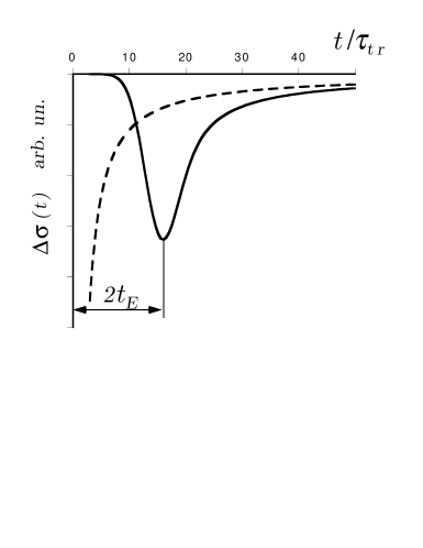
FIG. 1.: The weak localization correction to the conductivity in the time domain, $\Delta\sigma(t)=\int\frac{d\omega}{2\pi}\Delta\sigma(\omega)e^{-i\omega t}$ for the quantum chaos (solid line) and quantum disorder (dashed line) regimes. The developed theory is valid for $t\gtrsim t_{E}$. Solid curve is calculated for parameters $\lambda=4\lambda_{2}=1/\tau_{tr},\ \ln\left(a/\lambda_{F}\right)=7$.

The paper is arranged as follows. In Sec. II, we present the phenomenological derivation of Eq. (2). The explicit expression relating the weak localization correction to the solution of the Liouville equation will be derived in Sec. III. In Sec. IV, we will find the quantum corrections to the conductivity in the infinite chaotic system. Sec. V describes the effects of the magnetic field and finite phase relaxation time on the renormalization function. The conductance of the ballistic cavities is studied in Sec. VI. Our findings are summarized in Conclusion.

II Qualitative discussion

Classical diffusion equation is based on the assumption that at long time scales an electron looses any memory about its previous experience. However, during its travel, the electron may traverse the same spatial region and be affected by the same scatterer more than once. These two scattering events are usually considered independently, because with the dominant probability the electron enters this region having completely different momentum.

However, if we wish to find the probability $W_{0}(T,\rho_{0})$ for a particle to have the momentum opposite to the initial one, ${\bf p}(T)=-{\bf p}(0)$, (time $T$ is much larger than $\tau_{tr}$) and to approach its starting point at small distance $|{\bf r}(T)-{\bf r}(0)|=\rho_{0}\ll a$, we should take into account the fact that the motion of the particle at the initial and final stages are correlated. This is because the trajectory along which the particle moves on the final stage, $\left[{\bf r}(T-t),{\bf p}(T-t)\right]$ almost coincides with the trajectory particle moved along at the initial stage, $\left[{\bf r}(t),{\bf p}(t)\right]$, see Fig. 2. These correlations break down the description of this problem by the diffusion equation. The behavior of the distribution function for this case can be related to the Lyapunov exponent, and we now turn to the discussion of such a relation. (Relevance of $W_{0}(T,\rho_{0})$ to the weak localization correction will become clear shortly.)

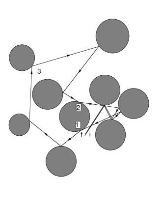
FIG. 2.: The classical trajectory corresponding to the probability of return at the initial point with the momentum opposite to the initial one. In the “Lyapunov region” the initial “i-1” and final “2-f” fragments of the trajectory are governed by the same potential.

The correlation of the motion at the final and initial stages can be conveniently characterized by two functions

$$\mbox{\boldmath$\rho$}(t)={\bf r}(t)-\!{\bf r}(T-t),\ \ {\bf k}(t)={\bf p}(T-t)+{\bf p}(t).$$ (4)

The classical equations of motion for these functions are

$$\displaystyle{\frac{\partial\mbox{\boldmath$\rho$}}{\partial t}=\frac{{\bf k}(t)}{m},}$$ (6)

$$\displaystyle{\frac{\partial{\bf k}}{\partial t}=\frac{\partial U[{\bf r}(T-t)]}{\partial{\bf r}}-\frac{\partial U[{\bf r}(t)]}{\partial{\bf r}}}$$ , (7)

where $U$ is the potential energy. If the distance $\rho$ is much larger than the characteristic spatial scale of the potential $a$, Eqs. (II) lead to the usual result $\langle\rho(t)\rangle\propto t^{1/2}$ at times $t$ much larger than $\tau_{tr}$. Situation is different, however, for $\rho\ll a$, where the diffusion equation is not applicable (we will call this region of the phase space the “Lyapunov region”). Thus, the calculation of function $W_{0}(T,\rho_{0})$ should be performed in two steps. First, we have to calculate the conditional probability $W(a,\rho_{0};t)$, which is defined so that the probability for the distance $\rho(t)$ to become larger than $a$ during the time interval $[t,\ t+\Delta t]$ is equal to $W(a,\rho_{0};t)\Delta t$ under the condition $\rho(0)=\rho_{0}$. Second, we have to obtain the probability $W_{D}(a,t)$ for the diffusively moving particle to approach its starting point to the distance of the order of $a$ (it corresponds to the fragment “1-3-2” in Fig. 2). Then, the function $W_{0}(T,\rho_{0})$ is given by

$$W_{0}(T,\rho_{0})=\int_{0}^{T}dtW_{D}(a,T-2t)W(a,\rho_{0};t).$$ (8)

Now, we perform the first step: finding of the probability $W(a,\rho_{0};t)$. We consider more general quantity $W(\rho,\rho_{0};t)$ for $\rho<a$. We expand the right hand side of Eq. (7) up to the first order in $\rho$ which yields

$$\frac{\partial{k}_{j}}{\partial t}=-{\cal M}_{ij}(t)\rho_{i},\quad{\cal M}_{ij}(t)\equiv\frac{\partial^{2}U[{\bf r}(t)]}{\partial{r}_{i}\partial{r}_{j}}.$$ (9)

It is easily seen from Eq. (9) and Fig. 2, that the change in the momentum $k$ during the scattering event is proportional to the distance $\rho$. On the other hand, it follows from Eq. (6) that the change in the value of $\rho$ between scattering events is proportional to $k$. Therefore, one can expect that the distance $\rho$ grows exponentially with time. In Appendix A we explicitly solve the model of weak dilute scatterers $l_{tr}\gg a$ and find the expression for the distribution function $W(\rho)=\left<\delta(t-t(\rho))\right>$, where $\left<...\right>$ means average over directions of ${\bf p}$. Here we present qualitative arguments which enable us to establish the form of the function $W$ for the general case.

We notice that, if matrix $\hat{\cal M}(t)$ does not depend on time, the solution of Eqs. (6) and (9) is readily available:

$$\rho(t)\simeq\rho(0)e^{\lambda t},$$ (10)

where the quantity $\lambda$ is related to the maximal negative eigenvalue of $\hat{\cal M}$. We will loosely call $\lambda$ the Lyapunov exponent. If $\hat{\cal M}$ varies with time, the solution of Eqs. (6) and (9) is not possible. We argue, however, that for the large time $t\gg\tau_{tr}$, this variation may be described by a random correction to the Lyapunov exponent:

$$\frac{d\ln\rho}{dt}=\lambda+\delta\lambda(t).$$ (11)

At time scale larger than $\tau_{tr}$ the correlation between the values of $\delta\lambda(t)$ at different moments of time can be neglected, $\left<\delta\lambda(t_{1})\delta\lambda(t_{2})\right>=\lambda_{2}\delta(t_{1}-t_{2})$, that immediately gives the log-normal form for the function $W$:

$$\displaystyle{W(\rho,\rho_{0};t)=\sqrt{\frac{\lambda^{3}}{2\pi\lambda_{2}\cal L(\rho)}}\exp\left[-\frac{\lambda\left({\cal L(\rho)}-\lambda t\right)^{2}}{2\lambda_{2}{\cal L(\rho)}}\right],}$$ (12)

$$\displaystyle{\hskip 113.81102pt{\cal L(\rho)}=\ln\rho/\rho_{0}.}$$ (13)

Formula (13) is valid in general case even though analytic calculation of the values of $\lambda$ and $\lambda_{2}$ (as well as of the diffusion constant) can be performed only for some special cases, e.g. for $l_{tr}\gg a$. For the antidot arrays, $\lambda$ is given by the inverse scattering time up to the factor of the order of $\ln(l_{tr}/a)$.[14] The model of the dilute weak scatterers is considered in Appendix A. The result is $\lambda,\lambda_{2}\simeq\tau_{tr}^{-1}(l_{tr}/a)^{2/3}$. In the ballistic billiards, coefficients $\lambda,\lambda_{2}$ are of the order of the inverse flying time across the system.

Equation (13) describes the distribution function only in the vicinity of its maximum, $\left|\ln\left({\rho}/{\rho_{0}}\right)-\lambda t\right|\lesssim\lambda t$. However, this result will be sufficient if time $T$ in Eq. (8) is large enough $T\gtrsim{\cal L}(a)/2\lambda$. At smaller times the probability of return is determined by the tail of the distribution function $W(\rho)$ which is by no means log-normal.

It is worth mentioning, that there is some arbitrariness in our choice of the initial conditions ${\bf p}(T)=-{\bf p}(0)$, $|{\bf r}(T)-{\bf r}(0)|=\rho_{0}$. The other possible choice is $|{\bf p}(T)+{\bf p}(0)|=k_{0}$, $|{\bf r}(T)-{\bf r}(0)|=0$. In this case, formula (13) remains valid upon the substitution $\rho_{0}\to ak_{0}/p(0)$.

Now we can find $W_{0}(T,\rho_{0})$ from Eq. (8). Substituting Eq. (13) into Eq. (8), we arrive to the result for the probability $W_{0}(T,\rho_{0})$:

$$\displaystyle{W_{0}(T,\rho_{0})=\int\frac{d\omega}{2\pi}W_{0}(\omega,\rho_{0})e^{-i\omega T}},$$ (14)

$$\displaystyle{W_{0}(\omega,\rho_{0})\!=\!W_{D}(\omega,a)\!\exp\left(\frac{2i\omega{\cal L}(a)}{\lambda}\!-\!\frac{2\omega^{2}\lambda_{2}{\cal L}(a)}{\lambda^{3}}\!\right),}$$ (15)

where $W_{D}(\omega,a)$ is the Fourier transform of the function $W_{D}(t,a)$. Function $W_{D}(a,\omega)=W_{D}(\omega;a\to l_{tr})W_{D}(\omega,l_{tr})$ is determined by two consecutive processes. First process, with the probability $W_{D}(\omega;a\to l_{tr})$, is the separation of the trajectories from distance $a$, at which they become independent to the distance larger than $l_{tr}$, where the diffusion equation is applicable. The characteristic time for such process is of the order of $\tau_{tr}$, and thus $W_{D}(\omega;a\to l_{tr})=1+{\cal O}(\omega\tau_{tr})$. The probability $W_{D}(\omega,l_{tr})$ is found by solving the standard diffusion equation. For the two-dimensional case, which will be most interesting for us, function $W_{D}(\omega,a)$ has the form

$$W_{D}(\omega,a)=\frac{1}{4\pi D}\ln\left(\frac{1}{\omega\tau_{tr}}\right),$$ (16)

where $D=v_{F}^{2}\tau_{tr}/2$ is the diffusion constant. Notice that this function does not depend on $a$. Expressions (16) and (13) are written with the logarithmic accuracy.

So far, we considered a purely classical problem. We found the probability for a particle, propagating in a classical disordered potential, to approach its starting point with the momentum opposite to its initial one. In the calculation of the classical kinetic coefficients (e.g. conductivity), the integration over all the direction of the momentum is performed. As the result, the peculiarities in the probability discussed above are washed out and do not appear in the classical kinetic coefficients. However, the function $W_{0}(\rho,t)$ plays very important role in the semiclassical approach to some quantum mechanical problems. One of such problems arose long time ago in the study[15] of break down of the method of the quasiclassical trajectories in the superconductivity theory[16]. Another problem is the weak localization in the quantum chaos and we turn to the study of this phenomenon now.

It is well known[17, 13, 18] that the probability $w$ for the particle to get from, say, point $i$ to point $f$, see Fig. 3a, can be obtained by, first, finding the quasiclassical amplitudes $A_{\alpha}$ for different paths connecting the points, and, then, by squaring the modulus of their sum:

$$w=\left|\sum_{\alpha}A_{\alpha}\right|^{2}=\sum_{\alpha}\left|A_{\alpha}\right|^{2}+\sum_{\alpha\neq\beta}A_{\alpha}A_{\beta}^{\ast}.$$ (17)

The first term in Eq. (17) is nothing else but the sum of the classical probabilities of the different paths, and the second term is due to the quantum mechanical interference of the different amplitudes. For generic pairs $\alpha,\beta$, the product $A_{\alpha}A_{\beta}^{\ast}$ oscillates strongly on the scale of the order of $\lambda_{F}$ as the function of the position of point $f$. This is because the lengths of the paths $\alpha$ and $\beta$ are substantially different. Because all the measurable quantities are averaged on the scale much larger than $\lambda_{F}$, such oscillating contributions can be neglected. There are pairs of paths, however, which are coherent. The example of such paths is shown in Fig. 3b, (paths $1$ and $2$). These paths almost always coincide. The only difference is that fragment $BEB$ is traversed in the opposite directions by trajectories $1$ and $2$. In the absence of the magnetic field and the spin-orbit interaction, the phases of the amplitudes $A_{1}$ and $A_{2}$ are equal because the lengths of the trajectories are close. The region, where the distance between trajectories $1,2$ is largest, see inset in Fig. 3b, deserves some discussion. At this point the directions of the paths at points $B_{1},B_{2}$ are almost opposite to those at points $B_{1}^{\prime},B_{2}^{\prime}$. Furthermore, the differences between lengths of paths $1$ and $2$ should not be larger than $\lambda_{F}$. It imposes certain restriction on angle $\delta\phi$ at which trajectory $2$ can intersect itself and on distance $\delta\rho$ to which the trajectory $1$ can approach itself. Simple geometric consideration, self-evident from inset in Fig. 3b, gives the estimate $\delta\rho\simeq\sqrt{\lambda_{F}l_{tr}}$ and $\delta\phi\simeq\sqrt{\lambda_{F}/l_{tr}}$, so that the uncertainty relation $\delta\phi\delta\rho\simeq\lambda_{F}$ holds. In other words, one of the trajectories should almost “graze itself” at the point ${B}$.

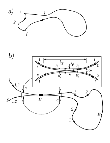
FIG. 3.: Examples of the classical (a) non-coherent and (b) coherent paths between points $i$ and $f$. The scatterers are not shown and the paths are straighten for clarity. Encircled is the Lyapunov region. The region of the quantum switch between trajectories (marked by the rectangular) is blown up on the inset.

The interference part of the contribution of the coherent pairs to the probability $w$, see Eq. (17) is of the same order as the classical probability for these trajectories. Therefore, the contribution of the interference effect to the conductivity $\sigma$ is proportional to the probability to find the trajectories similar to those from Fig. 3b. In order to calculate this probability, we use function $W_{0}(\rho,t)$ defined in the beginning of this section: the probability $dP$ for a trajectory to graze itself during the time interval $\left[t_{1},t_{1}+dt_{1}\right]$ is

$$dP_{1}=\delta\rho\delta\phi v_{F}dt_{1}W_{0}(\sqrt{\lambda_{F}l_{tr}},t_{1})=$$ (18)

$$\lambda_{F}v_{F}dt_{1}W_{0}(\sqrt{\lambda_{F}l_{tr}},t_{1}).$$ (19)

in two dimensions. We are, however, interested in the correction to the transport coefficients (such as the diffusion constant or the conductivity). These quantities are contributed mostly by the points $i,f$ located at the distance $\simeq l_{tr}$ from each other. Thus, in order to contribute to the diffusion constant or the conductivity, ends of the trajectories should separate from each other to the distance of the order of $a$, i.e. the trajectories should overcome the Lyapunov region one more time. The conditional probability $dP_{2}$ that the trajectories diverge at the distance $\sim a$ during the time interval $\left[t_{2},t_{2}+dt_{2}\right]$ under the condition that the self grazing occurred at moment $t_{1}$ is given by

$$dP_{2}=dt_{2}W(a,\sqrt{\lambda_{F}l_{tr}},t_{2}-t_{1}).$$ (20)

where $W$ is given by Eq. (13).

Summing over all the time intervals, we obtain for the quantum correction to the conductivity $\Delta\sigma$:

$$\hskip 56.9055pt\frac{\Delta\sigma}{\sigma}\approx-\int dP_{1}dP_{2}\approx$$ (21)

$$v_{F}\lambda_{F}\!\!\int_{0}^{\infty}\!\!\!\!dt_{2}\int_{0}^{\infty}\!\!\!\!dt_{1}W_{0}\!\left(\sqrt{\lambda_{F}l_{tr}},t_{1})\right)W\!\left(a,\sqrt{\lambda_{F}l_{tr}},t_{2}\right).$$ (22)

If the correction at finite frequency $\omega$ is needed, the time integration in Eq. (21) should be replaced with the Fourier transform over the total time of travel between points initial and final points $t=2t_{2}+t_{1}$ in Eq. (21). This yields

$${\Delta\sigma(\omega)}=-\frac{\sigma}{\pi\hbar\nu}W\left(a,\sqrt{\lambda_{F}l_{tr}},2\omega\right)W_{0}\left(\sqrt{\lambda_{F}l_{tr}},\omega\right),$$ (23)

where $\nu$ is the density of states per one spin. Coefficient in Eq. (23) and sign in Eqs. (21) and (23), known for the quantum disorder, will be reproduced for the quantum chaos in Sec. III. Substituting Eqs. (13) and (16) into Eq. (23) and using the Einstein relation ${\sigma}=se^{2}\nu D$, we arrive to the final result (2).[19]

III Weak localization in the quantum chaos

It follows from the previous discussion that the calculation of the quantum correction is related to the probability to find a classical trajectory with large correlated segments. Standard diagrammatic technique[4, 5, 13] is not convenient for this case because the averaging over the disorder potential is performed on the early stage, and including the additional correlations is technically difficult. That is why we will derive the expression for the quantum correction in terms of classical probabilities, which are the solutions of the Liouville equation in a given potential. This result is important on its own, because it provides a tool for the description of the quantum effects in the ballistic cavities. The averaging, then, can be performed only on the final stage of the calculations. For the sake of concreteness, we consider two-dimensional case; generalization to the other dimensions is straightforward. We will omit the Planck constant in all the intermediate calculations.

A Introduction of basic quantities

It is well known that transport coefficients can be calculated using the product of two exact Green functions $K_{\epsilon}$:

$$K_{\epsilon}(\omega;{\bf r}_{1},{\bf r}_{2},{\bf r}_{3},{\bf r}_{4})=G_{\epsilon+\frac{\omega}{2}}^{R}({\bf r}_{1},{\bf r}_{2})G_{\epsilon-\frac{\omega}{2}}^{A}({\bf r}_{3},{\bf r}_{4}).$$ (24)

Here $G^{R(A)}$ is the exact retarded (advanced) Green function of the electron in the disordered potential $U({\bf r})$ and it satisfies the equation

$$\left[\epsilon\pm i0-\hat{H}_{1}\right]G_{\epsilon}^{R,A}({\bf r}_{1},{\bf r}_{2})=\delta({\bf r}_{1}-{\bf r}_{2}),$$ (25)

where one-electron Hamiltonian is given by

$$\hat{H}_{1}=-\frac{\nabla_{{}_{1}}^{2}}{2m}+U({\bf r_{1}}).$$ (26)

For instance, the Kubo formula for the conductivity is

$$\displaystyle{\sigma^{\alpha\beta}\left(\omega;{\bf r}_{1},{\bf r}_{2}\right)=\frac{se^{2}}{4m^{2}}\int\frac{d\epsilon}{2\pi}\left(-\frac{\partial f}{\partial\epsilon}\right)\times}$$

$$\displaystyle{\left[\nabla_{{\bf r}_{1}}^{\alpha}-\nabla_{{\bf r}_{4}}^{\alpha}\right]\left[\nabla_{{\bf r}_{3}}^{\beta}-\nabla_{{\bf r}_{2}}^{\beta}\right]K_{\epsilon}(\omega;{\bf r}_{1},{\bf r}_{2},{\bf r}_{3},{\bf r}_{4})\left|{}_{\begin{array}[]{ll}{\bf r}_{4}={\bf r}_{1}\\ {\bf r}_{3}={\bf r}_{2}\end{array}}\right.,}$$

the expression for the polarization operator is

$$\Pi\left(\omega;{\bf r}_{1},{\bf r}_{2}\right) = s\left[\raisebox{0.0pt}[8.53581pt][8.53581pt]{$\nu$}\delta\left({\bf r}_{1}-{\bf r}_{2}\right)-\right.$$ (28)

$$i \!\!\omega\int\left.\displaystyle{\frac{d\epsilon}{2\pi}\frac{\partial f}{\partial\epsilon}}K_{\epsilon}(\omega;{\bf r}_{1},{\bf r}_{2},{\bf r}_{2},{\bf r}_{1})\right],$$ (29)

and so on. Here $f(\epsilon)=\left(e^{(\epsilon-\mu)/T}+1\right)^{-1}$ is the Fermi distribution function. Unfortunately, the exact calculation of $K$ is not possible and one has to resort on some approximations.

In general, function $K_{\epsilon}(\omega;{\bf r}_{1},{\bf r}_{2},{\bf r}_{3},{\bf r}_{4})$ oscillates rapidly with the distance between its arguments. It contains non-oscillating part only if its arguments are paired: ${\bf r}_{1}={\bf r}_{4},\ {\bf r}_{2}={\bf r}_{3}$ or, alternatively, ${\bf r}_{1}={\bf r}_{3},\ {\bf r}_{2}={\bf r}_{4}$. If they are not paired but still close to each other pairwise, then, it is very convenient to perform the Fourier transform over the difference of these close arguments:

$$\displaystyle{K_{\epsilon}(\omega;{\bf r}_{1},{\bf r}_{2},{\bf r}_{3},{\bf r}_{4})=\!\int\!\frac{d{\bf p}_{1}}{(2\pi)^{2}}\frac{d{\bf p}_{2}}{(2\pi)^{2}}e^{i{\bf p}_{1}\left({\bf r}_{1}-{\bf r}_{4}\right)}e^{i{\bf p}_{2}\left({\bf r}_{3}-{\bf r}_{2}\right)}}$$ (30)

$$\displaystyle{\quad\times K_{\epsilon}^{\cal D}\left(\omega;\ {\bf p}_{1},{\bf R}_{1};\ {\bf p}_{2},{\bf R}_{2}\right),}$$ (31)

$$\displaystyle{\quad\quad{\bf R}_{1}=\frac{{\bf r}_{1}+{\bf r}_{4}}{2},\ {\bf R}_{2}=\frac{{\bf r}_{2}+{\bf r}_{3}}{2}}.$$ (32)

or, alternatively,

$$\displaystyle{K_{\epsilon}(\omega;{\bf r}_{1},{\bf r}_{2},{\bf r}_{3},{\bf r}_{4})=\!\int\!\frac{d{\bf p}_{1}}{(2\pi)^{2}}\frac{d{\bf p}_{2}}{(2\pi)^{2}}e^{i{\bf p}_{1}\left({\bf r}_{1}-{\bf r}_{3}\right)}e^{i{\bf p}_{2}\left({\bf r}_{4}-{\bf r}_{2}\right)}}$$ (33)

$$\displaystyle{\quad\times K_{\epsilon}^{\cal C}\left(\omega;\ {\bf p}_{1},{\bf R}_{1};\ {\bf p}_{2},{\bf R}_{2}\right),}$$ (34)

$$\displaystyle{\quad\quad{\bf R}_{1}=\frac{{\bf r}_{1}+{\bf r}_{3}}{2},\ {\bf R}_{2}=\frac{{\bf r}_{2}+{\bf r}_{4}}{2}}.$$ (35)

Let us now derive the semiclassical equation for the function $K^{\cal D}$. From Eq. (25) and definition (24) we can write the equation for function $K$ in the form

$$\left[\omega-\hat{H}_{1}+\hat{H}_{4}\right]K_{\epsilon}(\omega;{\bf r}_{1},{\bf r}_{2},{\bf r}_{3},{\bf r}_{4})=$$ (36)

$$G_{\epsilon-\frac{\omega}{2}}^{A}({\bf r}_{3},{\bf r}_{4})\delta({\bf r}_{1}-{\bf r}_{2})-G_{\epsilon+\frac{\omega}{2}}^{R}({\bf r}_{1},{\bf r}_{2})\delta({\bf r}_{3}-{\bf r}_{4}).$$ (37)

If the distance $|r_{1}-r_{4}|$ is much smaller than the characteristic scale of the potential, we expand term $\hat{H}_{4}-\hat{H}_{1}$ in Eq. (37) in distance $|r_{1}-r_{4}|$, and perform the Fourier transform analogous to Eq. (32). The result can be expressed in terms of the Liouvillean operator $\hat{L}$:

$$i\left(\hat{H}_{1}-\hat{H}_{4}\right)\approx\hat{L}_{1}=\frac{\partial{\cal H}}{\partial{\bf p}_{1}}\cdot\frac{\partial}{\partial{\bf R}_{1}}-\frac{\partial{\cal H}}{\partial{\bf R}_{1}}\cdot\frac{\partial}{\partial{\bf p}_{1}}.$$ (38)

where ${\cal H}({\bf p},{\bf r})$ is the Hamiltonian function

$${\cal H}({\bf p},{\bf r})=\frac{{\bf p}^{2}}{2m}+U({\bf r}).$$ (39)

With the help of Eqs. (37), (38) and (32), we obtain

$$\left[-i\omega+\hat{L}_{1}\right]K_{\epsilon}^{\cal D}\left(\omega;\ {\bf p}_{1},{\bf R}_{1};\ {\bf p}_{2},{\bf R}_{2}\right)=$$ (40)

$$2\pi\delta\left[\epsilon-{\cal H}({\bf p}_{2},{\bf R}_{2})\right](2\pi)^{2}\delta({\bf p}_{1}-{\bf p}_{2})\delta({\bf R}_{1}-{\bf R}_{2}).$$ (41)

Delta-functions in the right hand side of Eq. (40) should be understood in a sense of there subsequent convolution with a function smooth on a spatial scale larger than $\lambda_{F}$. When deriving Eq. (40), we used the semiclassical approximation for the Green functions

$$G_{\epsilon}^{R,A}({\bf r}_{1},{\bf r}_{2})\!=\!\int\!\frac{d{\bf p}}{(2\pi)^{2}}\frac{e^{i{\bf p}\left({\bf r}_{1}-{\bf r}_{2}\right)}}{\epsilon-{\cal H}\left[{\bf p},\left({\bf r}_{1}+{\bf r}_{2}\right)/2\right]\pm i0}$$ (42)

in the right-hand side of Eq. (37) and neglected small frequency $\omega$ in comparison with the large energy $\epsilon\simeq E_{F}$.

Liouvillean operator (38) describes the motion of an electron in a stationary potential. Because the energy is conserved during such a motion, the function $K^{\cal D}$ can be factorized to the form

$$\displaystyle{K_{\epsilon}^{\cal D}\left(\omega;\ {\bf p}_{1},{\bf R}_{1};\ {\bf p}_{2},{\bf R}_{2}\right)={\cal D}_{\epsilon}\left(\omega;\ {\bf n}_{1},{\bf R}_{1};\ {\bf n}_{2},{\bf R}_{2}\right)\times}$$ (43)

$$\displaystyle{\quad\quad\frac{2\pi}{\nu}\delta\left[\epsilon-{\cal H}({\bf p}_{1},{\bf R}_{1})\right]\delta\left[\epsilon-{\cal H}({\bf p}_{2},{\bf R}_{2})\right]},$$ (44)

where diffuson ${\cal D}$ is a smooth function of the electron energy, ${\bf n}$ is the unit vector along the momentum direction, ${\bf p}=p_{F}{\bf n}={\bf n}\sqrt{2m\left[\epsilon-U({\bf r})\right]}$ and $\nu=m/2\pi$ is the density of states. Diffuson ${\cal D}_{\epsilon}$ is the solution of the equation

$$\left[-i\omega+\hat{L}_{1}\right]{\cal D}=\delta_{12},\quad\delta_{12}\equiv 2\pi\delta({\bf n}_{1}-{\bf n}_{2})\delta({\bf R}_{1}-{\bf R}_{2}).$$ (45)

It is important to emphasize that the diffuson ${\cal D}$ is a solution of the Liouville equation and not of the diffusion equation. In this sense, a more correct term for ${\cal D}$ is “Liouvillon”, however, we follow the terminology accepted in the theory of quantum disorder.

Let us consider the classical chaotic motion such that the time of the randomization of momentum direction is finite. At small $\omega$, which corresponds to the averaging over time scale much larger than the time of the momentum randomization, ${\cal D}_{\epsilon}$ averaged over small region of its initial conditions, satisfies the diffusion equation

$${\cal D}=\frac{1}{-i\omega-D\nabla^{2}},$$ (46)

where $D$ is the diffusion constant. The explicit relation of $D$ to the characteristics of the potential $U$ can be found in the limit of dilute scatterers $l_{tr}\gg a$: in this limit the diffusion constant is given by $D=v_{F}^{2}\tau_{tr}/2$. It is worth emphasizing that Eq. (46) itself does not require such a small parameter, and it is always valid at large spatial scales and small frequencies . We will ignore the possible islands in the phase space isolated from the rest of the system.

The semiclassical equation for function $K_{\epsilon}^{\cal C}$ from Eq. (35) is found in a similar fashion: in the absence of the magnetic field and spin-orbit scattering it reads

$$\left[-i\omega+\hat{L}_{1}\right]K_{\epsilon}^{\cal C}\left(\omega;\ {\bf p}_{1},{\bf R}_{1};\ {\bf p}_{2},{\bf R}_{2}\right)=$$ (47)

$$2\pi\delta\left[\epsilon-{\cal H}({\bf p}_{1},{\bf R}_{1})\right](2\pi)^{2}\delta({\bf p}_{1}-{\bf p}_{2})\delta({\bf R}_{1}-{\bf R}_{2}).$$ (48)

Function $K_{\epsilon}^{\cal C}$ can be factorized as

$$\displaystyle{K_{\epsilon}^{\cal C}\left(\omega;\ {\bf p}_{1},{\bf R}_{1};\ {\bf p}_{2},{\bf R}_{2}\right)={\cal C}\left(\omega;\ {\bf n}_{1},{\bf R}_{1};\ {\bf n}_{2},{\bf R}_{2}\right)\times}$$ (49)

$$\displaystyle{\quad\quad\frac{2\pi}{\nu}\delta\left[\epsilon-{\cal H}({\bf p}_{1},{\bf R}_{1})\right]\delta\left[\epsilon-{\cal H}({\bf p}_{2},{\bf R}_{2})\right]}.$$ (50)

Here Cooperon ${\cal C}_{\epsilon}$ is a smooth function of the electron energy satisfying the equation

$$\left[-i\omega+\hat{L}_{1}\right]{\cal C}=\delta_{12}.$$ (51)

Similar to the diffuson, the Cooperon, averaged over small region of its initial conditions, is a self-averaging quantity at large distances and small frequencies and in the absence of magnetic field and spin-orbit scattering, it can be described by the expression analogous to Eq. (46):

$${\cal C}=\frac{1}{-i\omega-D\nabla^{2}}.$$ (52)

B Quantum corrections to classical probabilities.

So far, we considered the lowest classical approximation, in which the classical probabilities were determined by the deterministic equations of the first order. However, the potential $U$ contains not only the classical smooth part which is taken into account by the Liouville equation, but also the part, responsible for the small angle diffraction. Quantum weak localization correction originates from the interference of the diffracted electron waves. The interference of the waves diffracted at different locations is added. It results, as we will show below, the quantum correction ceases to depend upon the details of the diffraction mechanism and becomes universal. The only quantity which depends on the diffraction angle is the time it takes to establish this universality. We will show, see also Sec. II, that the dependence of this time on the diffraction angle is only logarithmical. Therefore, with the logarithmic accuracy, we can include the effect of this diffraction into the classical Liouville equation by any convenient method, provided that we do it consistently for all the quantities and preserve the conservation of the number of particles.

We will model the diffraction by adding the small amount of the quantum small angle scatterers to the LHS of the Schrödinger equation (25). The effect of these scatterers will be twofold: 1) They will smoothen the sharp classical probabilities; 2) They will induce interaction between the diffuson and Cooperon modes, that results in the weak localization correction. Finally, the strength and the density of these scatterers will be adjusted so that the angle at which the classical probability is smeared during the travel to the distance $a$ is equal to the genuine diffraction angle $\sqrt{\lambda_{F}/a}$. This procedure is legitimate because, as we already mentioned, the dependence of weak localization correction on the diffraction angle is only logarithmical.

It is worth emphasizing, that even though weak localization correction takes its origin at the very short linear scale (ultraviolet cut-off), the value of this correction at very large distances does not depend on this cut-off at all. Such phenomena are quite typical in physics, (e.g. in the theory of turbulence, theory of strong interaction, or in the Kondo effect).

Let us now implement the procedure. Consider a single impurity located at the point ${\bf s}$, and creating the potential $V({\bf r})=V_{0}({\bf s-r})$, so that the potential part of the Hamiltonian (26) is now given by $U({\bf r})+V({\bf r})$. The characteristic size of this potential, $d$, is much larger than $\lambda_{F}$ but much smaller than $a$. Our goal is to find the correction to Eqs. (45) and (51) in the second order of perturbation theory in potential $V$. (Correction of the first order vanishes if ${\cal D}$ and ${\cal C}$ are functions smooth on the spatial scale $d$.) In this order, correction to function (24) has the form

  

$$\displaystyle{\delta K\left({\bf r}_{1},{\bf r}_{2},{\bf r}_{3},{\bf r}_{4}\right)=\int d{\bf r}_{5}{\bf r}_{6}\left[G^{R}({\bf r}_{1},{\bf r}_{5})V({\bf r}_{5})G^{R}({\bf r}_{5},{\bf r}_{2})G^{A}({\bf r}_{3},{\bf r}_{6})V({\bf r}_{6})G^{A}({\bf r}_{6},{\bf r}_{4})\right.+}$$ (53)

$$\displaystyle{\left.\quad G^{R}({\bf r}_{1},{\bf r}_{5})V({\bf r}_{5})G^{R}({\bf r}_{5},{\bf r}_{6})V({\bf r}_{6})G^{R}({\bf r}_{6},{\bf r}_{2})G^{A}({\bf r}_{3},{\bf r}_{4})+G^{R}({\bf r}_{1},{\bf r}_{2})G^{A}({\bf r}_{3},{\bf r}_{5})V({\bf r}_{5})G^{A}({\bf r}_{5},{\bf r}_{6})V({\bf r}_{6})G^{R}({\bf r}_{6},{\bf r}_{2})\right],}$$ (54)

                                                                                

where Green functions are the solutions of Eq. (25) without the impurity potential $V$. We will omit the energy arguments in the Green function, implying everywhere that the energies for the retarded and advanced Green functions are $\epsilon+\omega/2$ and $\epsilon-\omega/2$ respectively.

In order to find the correction to the diffuson, we consider the points $r_{1},r_{4}$ and $r_{2},r_{3}$ in Eq. (53) which are close to each other pairwise, perform the Fourier transform defined by Eq. (32), and express the RHS of Eq. (53) in terms of the diffusons and Cooperons. We demonstrate the calculation by evaluating the second term in the RHS of Eq. (53), let us denote it by $\delta K_{2}$.

Consider the product $G^{R}({\bf r}_{1},{\bf r}_{5})G^{A}({\bf r}_{3},{\bf r}_{4})$, points $r_{1},r_{4}$ are close to each other, but points $r_{5},r_{3}$ are not. It means that for calculation of such a product we can not use the semiclassical approximation (42) for the RHS of Eq. (37) but sill can use the expansion (38) for the LHS of Eq. (37). Solving Eq. (37) with the help of Eq. (45), we obtain

  

$$\displaystyle{G^{R}({\bf r}_{1},{\bf r}_{5})G^{A}({\bf r}_{3},{\bf r}_{4})=\frac{i}{\nu}\int d{\bf r}_{7}{\bf r}_{8}\int\frac{d{\bf p}_{1}}{(2\pi)^{2}}\frac{d{\bf p}_{2}}{(2\pi)^{2}}e^{i{\bf p}_{1}({\bf r}_{1}-{\bf r}_{4})-i{\bf p}_{2}({\bf r}_{7}-{\bf r}_{8})}{\cal D}\left({\bf n}_{1},\frac{{\bf r}_{1}+{\bf r}_{4}}{2};{\bf n}_{2},\frac{{\bf r}_{7}+{\bf r}_{8}}{2}\right)\times}$$ (55)

$$\displaystyle{\left[G^{R}({\bf r}_{7},{\bf r}_{5})\delta({\bf r}_{8}-{\bf r}_{3})-G^{A}({\bf r}_{3},{\bf r}_{8})\delta({\bf r}_{7}-{\bf r}_{5})\right]\delta\left[{\cal H}\left({\bf p}_{1},\frac{{\bf r}_{1}+{\bf r}_{4}}{2}\right)-{\cal H}\left({\bf p}_{2},\frac{{\bf r}_{7}+{\bf r}_{8}}{2}\right)\right],}$$ (56)

                                                                                

with ${\cal H}({\bf p},{\bf r})$ being the Hamilton function (39). We will omit the frequency argument in the diffusons and Cooperons, implying everywhere that it equals to $\omega$.

We substitute Eq. (55) into the second term in the LHS of Eq. (53). We neglect the product of three retarded Green functions because this product is a strongly oscillating function of its arguments and vanishes after the averaging on a spatial scale larger than $\lambda_{F}$. The remaining product $G^{R}({\bf r}_{6},{\bf r}_{2})G^{A}({\bf r}_{3},{\bf r}_{8})$ is approximated by the expression similar to Eq. (55) because points ${\bf r}_{2}$ and ${\bf r}_{3}$ are close to each other. Neglecting, once again, the product of two retarded Green functions and performing the Fourier transform over the differences $r_{1}-r_{4}$ and $r_{2}-r_{3}$, we find

  

$$\displaystyle{\delta{\cal D}_{2}(1,2)=-\int\!\!d{\bf r}_{3}d{\bf r}_{4}d{\bf R}_{3}d{\bf R}_{4}\int\!\!\frac{d{\bf p}_{3}}{(2\pi)^{2}}\frac{d{\bf p}_{4}}{(2\pi)^{2}}e^{-i{\bf p}_{3}{\bf r}_{3}+i{\bf p}_{4}{\bf r}_{4}}{\cal D}\left(1;3\right){\cal D}\left(4;2\right)G^{R}\left({\bf r}_{3}^{+},{\bf r}_{4}^{+})G^{A}({\bf r}_{4}^{-},{\bf r}_{3}^{-}\right)\frac{V({\bf r}_{3}^{+})V({\bf r}_{4}^{+})}{2\pi\nu},}$$ (57)

$$\displaystyle{\delta K_{2}\left({\bf r}_{1}^{+},{\bf r}_{2}^{+},{\bf r}_{2}^{-},{\bf r}_{1}^{-}\right)={2\pi\nu}\int\frac{d{\bf n}_{1}}{(2\pi)}\frac{d{\bf n}_{2}}{(2\pi)}e^{ip_{F}{\bf n}_{1}{\bf r}_{1}-ip_{F}{\bf n}_{2}{\bf r}_{2}}\delta{\cal D}_{2}\left(1,2\right),}$$ (58)

Here we introduced the short hand notation $j\equiv({\bf n}_{j},{\bf R}_{j})$ and ${\bf r}_{j}^{\pm}={\bf R}_{j}\pm\frac{{\bf r}_{j}}{2}$.

What remains is to find the semiclassical expression for the product $G^{R}G^{A}$ in Eq. (58). We notice that the points ${\bf r}_{3}^{+},{\bf r}_{4}^{+}$ lie within the radius of the potential $V(r)$. In order for the product $G^{R}G^{A}$ in Eq. (58) not to vanish, the points ${\bf r}_{3}^{-},{\bf r}_{4}^{-}$ must be close to the points ${\bf r}_{3}^{+},{\bf r}_{4}^{+}$. Because all the four points are close to each other, one can write, cf. Eq. (35),

$$G^{R}\left({\bf r}_{3}^{+},{\bf r}_{4}^{+})G^{A}({\bf r}_{4}^{-},{\bf r}_{3}^{-}\right)=\nu^{2}\int\!{d{\bf n}_{4}}{d{\bf n}_{5}}\ \theta\ [{\bf n}_{4}({\bf r}_{3}^{+}-{\bf r}_{4}^{+})]\ \theta\ [{\bf n}_{5}({\bf r}_{4}^{-}-{\bf r}_{3}^{-})]\ e^{ip_{F}{\bf n}_{4}({\bf r}_{3}^{+}-{\bf r}_{4}^{+})+ip_{F}{\bf n}_{5}({\bf r}_{3}^{-}-{\bf r}_{4}^{-})}+$$ (59)

$$\frac{\nu}{2\pi}\int{d{\bf n}_{4}}{d{\bf n}_{5}}e^{ip_{F}{\bf n}_{4}({\bf r}_{3}^{+}-{\bf r}_{4}^{-})+ip_{F}{\bf n}_{5}({\bf r}_{3}^{-}-{\bf r}_{4}^{+})}{\cal C}\left({\bf n}_{4},\frac{{\bf r}_{3}^{+}+{\bf r}_{4}^{-}}{2};{\bf n}_{5},\frac{{\bf r}_{3}^{-}-{\bf r}_{4}^{+}}{2}\right).$$ (60)

                                                                                

Here, the first term is the explicitly separated contribution of the short straight line trajectories connecting points $r_{1},r_{2}$ and $r_{3},r_{4}$. These short trajectories can be well described by the Cooperon or by the diffuson. The second term describes the contribution of all the other trajectories connecting these points. It can be shown by explicit calculation that the representation of Eq. (60) in terms of the diffuson only would lead to the loss of this second term. This is because the Cooperon describes the interference effects corresponding to the oscillating part of the diffuson which is lost in the semiclassical approximation (45).

Now, we are ready to find the correction coming from the single quantum scatterer. We substitute Eq. (60) into Eq. (58) and perform the integration while neglecting the dependence of the diffusons and Cooperon on their spatial coordinates on the scale of the order of the scatterer size. We consider the remaining two terms in Eq. (53) in a similar manner. The overall result is

$$\displaystyle{\delta{\cal D}=\delta{\cal D}^{St}+\delta{\cal D}^{I},}$$ (61)

$$\displaystyle{\delta{\cal D}^{St}(1,2)=\int d3d4{\cal P}_{s}(3,4){\cal D}(1,3)\left[{\cal D}(4,2)-{\cal D}(3,2)\right],}$$ (62)

$$\displaystyle{\delta{\cal D}^{I}(1,2)=\int d3d4{\cal P}_{s}(3,4)\frac{{\cal C}(3,\bar{4})}{2\pi\nu}\times}$$ (63)

$$\displaystyle{\hskip 42.67912pt\left[{\cal D}(1,3)-{\cal D}(1,4)\right]\left[{\cal D}(\bar{3},2)-{\cal D}(\bar{4},2)\right].}$$ (64)

Here we use the short hand notation $j\equiv({\bf n}_{j},{\bf R}_{j})$, integration over the phase space on the energy shell is defined as $dj\equiv d{\bf n}_{j}d{\bf R}_{j}/2\pi$, the time reversed coordinate $\bar{j}$ is given by $\bar{j}\equiv(-{\bf n}_{j},{\bf R}_{j})$, and the kernel ${\cal P}$ describing the scattering by an impurity is

$\displaystyle{\cal P}_{s}(1,2)\!=\!2\pi\nu\delta({\bf s}-{\bf R}_{1})\delta({\bf s}-{\bf R}_{2})\left|\int\!d{\bf r}e^{ip_{F}{\bf r}({\bf n}_{1}-{\bf n}_{2})}V({\bf r})\right|^{2}\!.$

The first term $\delta D^{St}$ in Eq. (61) coincides with that obtained for otherwise free moving electrons. The second term, $\delta D^{I}$, describes the interference effect arising because the chaotically moving in classical potential $U(r)$ electron may return to the vicinity of the impurity one more time.

The correction to the Cooperon due to the single impurity can be obtained from Eq. (53) by considering close pairs $r_{1},r_{3}$ and $r_{2},r_{4}$; this results in the expression similar to Eq. (61) with the replacement ${\cal D}\leftrightarrow{\cal C}$.

So far, we considered the correction due to a single weak impurity. If the number of these impurities is large, we can, in the lowest approximation, consider the contributions from the different impurities independently of each other, by the substitution to the RHS of Eqs. (61) of the diffusons and Cooperons renormalized by all the other impurities. As the result, we arrive to the Boltzmann-like equations for the diffuson and Cooperon

  

$$\displaystyle{\left[-i\omega+\hat{L}_{1}\right]{\cal D}(1,2)=\delta_{12}+\sum_{\bf s}\int d3{\cal P}_{s}(1,3)\left\{\left[{\cal D}(3,2)-{\cal D}(1,2)\right]+\left[{\cal D}(\bar{1},2)-{\cal D}(\bar{3},2)\right]\frac{{\cal C}(1,\bar{3})+{\cal C}(3,\bar{1})}{2\pi\nu}\right\}}$$ (66)

$$\displaystyle{\left[-i\omega+\hat{L}_{1}\right]{\cal C}(1,2)=\delta_{12}+\sum_{\bf s}\int d3{\cal P}_{s}(1,3)\left\{\left[{\cal C}(3,2)-{\cal C}(1,2)\right]+\left[{\cal C}(\bar{1},2)-{\cal C}(\bar{3},2)\right]\frac{{\cal D}(1,\bar{3})+{\cal D}(3,\bar{1})}{2\pi\nu}\right\}}$$ (67)

                                                                                

where the notation for the coordinates $j,\bar{j}$ was introduced after Eq. (61), and the $\delta$ - symbol was defined in Eq. (45).

Assuming that the distribution of the quantum impurities is uniform with the density $n_{i}$, we can make the continuous approximation and replace $\sum_{\bf s}\to n_{i}\int d{\bf s}$ in the RHS of Eqs. (III B). Finally, taking into account that the scattering angle is small, we reduce Eqs. (III B) to a differential form. Equation (66) becomes

$$\left[-i\omega+\hat{L}_{1}-\frac{1}{\tau_{q}}\frac{\partial^{2}}{\partial\phi^{2}_{1}}\right]{\cal D}(1)=\delta_{12}-\frac{\partial}{\partial\phi_{1}}\frac{{\cal C}(1,\bar{1})}{\pi\nu\tau_{q}}\frac{\partial}{\partial\phi_{1}}{\cal D}(\bar{1})$$ (69)

Here, angle $\phi_{j}$ is defined so that ${\bf n}_{j}=(\cos\phi_{j},\sin\phi_{j})$, the notation for the coordinates $j\equiv({\bf n}_{j},{\bf R}_{j}),\ \bar{j}\equiv(-{\bf n}_{j},{\bf R}_{j})$, is the same as in Eq. (61), and the $\delta$ - symbol was defined in Eq. (45). The second argument is the same for all the diffusons in Eq. (69) and that is why we omitted it. Analogously, Eq. (67) reduces to

$$\left[-i\omega+\hat{L}_{1}-\frac{1}{\tau_{q}}\frac{\partial^{2}}{\partial\phi^{2}_{1}}\right]{\cal C}(1)=\delta_{12}-\frac{\partial}{\partial\phi_{1}}\frac{{\cal D}(1,\bar{1})}{\pi\nu\tau_{q}}\frac{\partial}{\partial\phi_{1}}{\cal C}(\bar{1})$$ (70)

The second argument is the same for all the Cooperons in Eq. (70) and it is omitted. Quantum transport life time in Eqs. (III B) is given by

$\displaystyle\frac{1}{\tau_{q}}=\!2\pi\nu n_{i}\int\frac{d\phi}{2\pi}\frac{\phi^{2}}{2}\left|\int\!d{\bf r}e^{ip_{F}{\bf n}{\bf r}\phi}V({\bf r})\right|^{2}\!.$

Equations (III B) describe how the classical Liouville equation changes under the effect of the small angle scattering (diffraction). We see that the quantum effects result in two contributions to the Liouville equation. First contribution provides the angular diffusion and, thus, it leads to the smearing of the sharp classical probabilities. Usually, for the calculation of the transport coefficients, such as the diffusion constant or the conductivity, the averaging over the initial and final coordinates is performed anyway. Therefore, the angular diffusion itself provides only negligible correction to the classical transport coefficients which are controlled by classical potential $U$. On the contrary, the second contribution giving the quantum correction [last terms in the RHS of Eq. (69)] is proportional to the classical probability $C(\bar{1},1)$ where the initial and finite points of the phase space are related by the time inversion. In the absence of the spreading due to the angular diffusion, $\tau_{q}\to\infty$, this probability vanishes identically, see Sec. II. In order to obtain the correction at finite time (or finite frequency), one must keep $\tau_{q}$ finite even in the final results.

Let us estimate the value one should ascribe to $\tau_{q}$ for the description of the diffraction effects in the system. As we already discussed, for the calculation with the logarithmic accuracy, we do not need the numerical coefficient. The parametric dependence of $\tau_{q}$ can be established by using the following argument. Consider two independent electrons, starting with the same initial conditions. If there were no diffraction, they would propagate together forever. Due to the angular diffusion (diffraction), the directions of these trajectories deviates first $\propto\sqrt{t}$ and then exponentially, $\frac{d\langle\delta\phi^{2}\rangle}{dt}\approx 2\lambda\langle\delta\phi^{2}\rangle+\frac{1}{2\tau_{q}}$, where angle $\delta\phi$ stands for the angle between the momenta of two electrons, and $\lambda$ is the Lyapunov exponent. It yields $\langle\delta\phi^{2}(t)\rangle\approx(4\lambda\tau_{q})^{-1}\left(e^{2\lambda t}-1\right)$. Thus, the characteristic time during which the angular diffusion switches to the exponential growth is always $t_{e}\simeq 1/\lambda$. On the other hand, quantum spreading of the wave packet during this time interval is given by $\delta x^{2}\simeq\lambda_{F}v_{F}t_{e}$. Taking into account the relation $\delta x\simeq\phi t_{e}v_{F}$, we find $t_{e}/\tau_{q}\simeq\lambda_{F}/(v_{F}t_{e})$. It yields the estimate for the quantum transport time entering into Eqs. (III B) corresponding to the small angle diffraction

$$\frac{1}{\tau_{q}}\simeq\lambda^{2}\frac{\lambda_{F}}{v_{F}}.$$ (71)

It is important to emphasize that the very same $\tau_{q}$ enters into the angular diffusion term and into the diffuson-Cooperon interaction. This circumstance is extremely crucial for the universality of the quantum correction at large time ($\omega\to 0$), even though parameter $\tau_{q}$ itself does not enter into the result, see Sec. IV.

Let us now turn to the calculation of the lowest quantum correction to the diffuson. Taking into account the last term in the RHS of Eq. (69) in the first order of perturbation theory, we obtain

$${\cal D}(1,2)={\cal D}^{0}(1,2)+\Delta{\cal D}(1,2);$$ (73)

$$\Delta{\cal D}(1,2)=\int d3\frac{{\cal C}^{0}(3,\bar{3})}{\pi\nu\tau_{q}}\frac{\partial{\cal D}^{0}(1,3)}{\partial\phi_{3}}\frac{\partial{\cal D}^{0}(\bar{3},2)}{\partial\phi_{3}};$$ (74)

$$\left[-i\omega+\hat{L}_{1}-\frac{1}{\tau_{q}}\frac{\partial^{2}}{\partial\phi^{2}_{1}}\right]{\cal D}^{0}(1,2)=\delta_{12};$$ (75)

$$\left[-i\omega+\hat{L}_{1}-\frac{1}{\tau_{q}}\frac{\partial^{2}}{\partial\phi^{2}_{1}}\right]{\cal C}^{0}(1,2)=\delta_{12},$$ (76)

where $j\equiv({\bf n}_{j},{\bf R}_{j})$, integration over the phase space on the energy shell is defined as $dj\equiv d{\bf n}_{j}d{\bf R}_{j}/2\pi$, the time reversed coordinate $\bar{j}$ is given by $\bar{j}\equiv(-{\bf n}_{j},{\bf R}_{j})$, and the $\delta$ - symbol was defined in Eq. (45).

Equation (74) can be rewritten in a different form. Even though more lengthy than Eq. (74), this form turns out to be more convenient for further applications:

$$\Delta{\cal D}(1,2)={\cal D}^{0}(1,\bar{2})\frac{{\cal C}^{0}(\bar{2},2)}{2\pi\nu}+\frac{{\cal C}^{0}(1,\bar{1})}{2\pi\nu}{\cal D}^{0}(\bar{1},2)$$ (77)

$$+\int d3{\cal D}^{0}(1,3){\cal D}^{0}(\bar{3},2)\left[2i\omega-\hat{L}_{3}+\frac{1}{\tau_{q}}\frac{\partial^{2}}{\partial\phi^{2}_{3}}\right]\frac{{\cal C}^{0}(3,\bar{3})}{2\pi\nu}.$$ (78)

In order to derive Eq. (77) from Eq. (74), we subtracted from the RHS of Eq. (77) the expression

$\displaystyle\int d3\hat{L}_{3}\left[\frac{{\cal C}(3,\bar{3})}{2\pi\nu}{\cal D}(1,3){\cal D}(\bar{3},2)\right],$which vanishes because integrand is the total derivative along the classical trajectory. Then, we integrated Eq. (74) by parts and, with the help of Eq. (75), we arrived to Eq. (77).

Equations (74) and (77) are the main results of this section. They give the value of the lowest quantum correction to the classical correlator in terms of the non-averaged solutions of the Liouville equation (with small angular diffraction added) for a given system. Besides the found correction, there exist the other corrections [e.g. from the higher terms in the expansion (38)], however, Eqs. (74) and (77) are dominant at low frequencies. The quantum mesoscopic fluctuations are neglected in Eqs. (74) and (77), which implies either the temperature is high enough or the averaging over the position of the Fermi level is performed. Then, if the relevant time and spatial scales are large, the quantum correction becomes a self-averaging quantity expression for which will be obtained in the next section.

IV Averaged quantum corrections

We will consider the quantum correction at large distance and time scales. In this case, the classical probability does not depend on the direction of the momentum and it is given by Eq. (46). Our goal now is to find the expression for the quantum correction in the same approximation. We will bear in mind the systems in which the diffusion constant is large enough, $D/av_{F}\gtrsim 1$. It is the case for the antidot arrays. The conductance of the net of the ballistic cavities requires a separate consideration.

For the calculation we use Eq. (77). While performing the averaging, we make use of the fact that the Cooperon part of the expression can be averaged independently on the diffuson part. This is because the classical trajectories corresponding to these quantities lie essentially in the different spatial regions, (see e.g. Fig. 3b, where segments $iB$ and $fB$ correspond to diffusons and segment $BEB$ corresponds to the Cooperon) and, therefore, they are governed by the different potentials and are not correlated. Performing such an averaging, we obtain from Eq. (77):

$$\Delta{\cal D}(1,2)=\left[\raisebox{0.0pt}[8.53581pt][8.53581pt]{$\langle{\cal D}^{0}(1,\bar{2})\rangle+\langle{\cal D}^{0}(\bar{1},{2})\rangle+$}\right.$$ (79)

$$\hskip 56.9055pt\left.2i\omega\int d3\langle{\cal D}^{0}(1,3){\cal D}^{0}(\bar{3},2)\rangle\right]\displaystyle{\frac{\langle{\cal C}^{0}(1,\bar{1})\rangle}{2\pi\nu}.}$$ (80)

where $\langle\dots\rangle$ stands for the averaging either over the realization of potential $U$ or over the position of the “center of mass” of the Cooperon and diffuson. The last two terms in brackets in Eq. (77) vanish after averaging because the averaged cooperon does not depend on the coordinates ${\bf n}_{3},{\bf R}_{3}$.

On the other hand, as we have already explained in Sec. II, the correlations in the motion of both ends of the Cooperon can not be neglected. The same is also true about the correlation between motion of the ends $3$ and $\bar{3}$ in the third term of Eq. (77). In what follows, we will separate the description of the problem into the Lyapunov and diffusion regions. It will be done in subsections IV A and IV B for the Cooperon and diffusons respectively, and the resulting correction to the conductivity will be found in subsection IV C. The description of the Lyapunov region is presented in subsections IV D and IV E.

A Cooperon in the diffusive and Lyapunov regions

In order to find $\langle{\cal C}^{0}(1,\bar{1})\rangle$ we consider more general quantity ${C}(\phi,\rho)$ defined as

$${C}(\phi,\rho)=\frac{1}{S}\int\frac{d{\bf R}d{\bf n}}{2\pi}{\cal C}^{0}\left({\bf n}^{+},{\bf R}^{-};-{\bf n}^{-},{\bf R}^{+}\right),$$ (81)

$${\bf n}^{\pm}={\bf n}\cos\frac{\phi}{2}\pm\left[{\bf n}\times{\bf l}_{z}\right]\sin\frac{\phi}{2},\ {\bf R}^{\pm}={\bf R}\pm\frac{\rho}{2}\left[{\bf n}^{\pm}\times{\bf l}_{z}\right],$$ (82)

where $S$ is the area of the sample, and ${\bf l}_{z}$ is the unit vector perpendicular to the plane. Function ${C}(0,0)$ coincides with the necessary quantity $\langle{\cal C}^{0}(1,\bar{1})\rangle$.

It is easy to find ${C}(\phi,\rho)$ in the diffusion region. At $\rho\gtrsim l_{tr}$, it is given by

$${C}\left(\phi,\rho\right)=\frac{1}{-i\omega-D\nabla^{2}_{\rho}}.$$ (83)

At $\rho<\sqrt{D/\omega}$ the Cooperon depends only logarithmically on $\rho$ and at $a\lesssim\rho\lesssim l_{tr}$, it becomes independent of $\rho$. With the logarithmic accuracy, we have

$${C}\left(\phi,\rho\right)\approx\frac{1}{4\pi D}\ln\left(\frac{1}{\omega\tau_{tr}}\right),\quad\rho\gtrsim a.$$ (84)

Equation (84) serves as the boundary condition for ${C}\left(\phi,\rho\right)$ at the boundary between the diffusive and Lyapunov regions:

$${C}\left(\phi,\rho=a\ {\rm sign}\phi\right)\approx\frac{1}{4\pi D}\ln\left(\frac{1}{\omega\tau_{tr}}\right).$$ (85)

Meaning of Eq. (85) is that both ends of the Cooperon enter into the Lyapunov region with the random momenta, and thus the probability of this entrance is given by the solution of the diffusion equation.

The next step is to find ${C}(\phi,\rho)$ in the Lyapunov region. We add to Eq. (76), the equation conjugate to it, which gives

$$\left[-2i\omega+\hat{L}_{1}+\hat{L}_{2}-\frac{1}{\tau_{q}}\frac{\partial^{2}}{\partial\phi_{1}^{2}}-\frac{1}{\tau_{q}}\frac{\partial^{2}}{\partial\phi_{2}^{2}}\right]{\cal C}^{0}(1,\bar{2})=2\delta_{1\bar{2}}.$$ (86)

Formula (86) enables us to find the equation for quantity ${\cal C}^{0}\left({\bf n},{\bf R};\phi,\rho\right)\equiv{\cal C}^{0}\left({\bf n}^{+},{\bf R}^{-};-{\bf n}^{-},{\bf R}^{+}\right)$ from Eq. (81). Expanding potential $U$ up to the first order in $\rho$, and using the fact that the angle $\phi$ is small, we obtain

$$\left[-2i\omega+\hat{L}_{c}+\hat{L}_{r}-\frac{1}{2\tau_{q}}\frac{\partial^{2}}{\partial\phi^{2}}\right]{\cal C}^{0}\left({\bf n},{\bf R};\phi,\rho\right)=0.$$ (87)

Here operator

$$\hat{L}_{c}=v_{F}{\bf n}\cdot\frac{\partial}{\partial{\bf R}}-\frac{\partial U({\bf R})}{\partial{\bf R}}\cdot\frac{\partial}{\partial{\bf P}}$$ (88)

describes the motion of the “center of mass” of the Cooperon along a classical trajectory and operator $\hat{L}_{r}$ characterizes how the distance between the ends changes in a course of this motion:

$$\hat{L}_{r}=-v_{F}\phi\frac{\partial}{\partial\rho}+\frac{\partial^{2}U}{p_{F}\partial R_{\perp}^{2}}\rho\frac{\partial}{\partial\phi}.$$ (89)

with $R_{\perp}$ being the projection of ${\bf R}$ onto the direction perpendicular to ${\bf n}$. In Eq. (87), we neglected the effect of the angular diffusion on the motion of the center of mass because the averaging over the position of the center of mass ${\bf n,\ R}$ is performed in Eq. (81) anyway.

Now, we have to find function $C(\rho,\phi)$ in the Lyapunov region, satisfying the boundary condition given by Eq. (85) and consistent with Eqs. (81) and (87). Solution can be represented in a compact form analogous to Eq. (8)

$${C}\left(\phi,\rho\right)=\frac{w\left(\omega;\phi,\rho\right)}{4\pi D}\ln\left(\frac{1}{\omega\tau_{tr}}\right).$$ (90)

Function $w\left(\omega;\phi,\rho\right)$ is defined as

$$w\left(\omega;\phi,\rho\right)=\frac{1}{S}\int\frac{d{\bf R}d{\bf n}}{2\pi}W\left(\omega;{\bf n},{\bf R};\phi,\rho\right),$$ (91)

where $S$ is the area of the sample and $W$ is the solution of the equation

$$\left[-2i\omega+\hat{L}_{c}+\hat{L}_{r}-\frac{1}{2\tau_{q}}\frac{\partial^{2}}{\partial\phi^{2}}\right]W\left(\omega;{\bf n},{\bf R};\phi,\rho\right)=0,$$ (92)

supplied with the boundary condition

$$W\left(\omega;{\bf n},{\bf R};\phi,\rho=a\ {\rm sign}\phi\right)=1.$$ (93)

The necessary quantity $\langle{\cal C}^{0}(1,\bar{1})\rangle$ is, thus, found by putting $\rho,\phi=0$ in Eq. (90)

$$\langle{\cal C}^{0}(1,\bar{1})\rangle=\frac{w\left(\omega;0,0\right)}{4\pi D}\ln\left(\frac{1}{\omega\tau_{tr}}\right).$$ (94)

B Diffusons in the diffusive and Lyapunov regions.

In this subsection we find the average $\int d3\langle{\cal D}^{0}(1,3){\cal D}^{0}(\bar{3},2)\rangle$ entering into Eq. (80). We use the procedure similar to the calculation of the Cooperon in the previous subsection. We consider more general quantities $M,\ {\cal M}$ defined as

$${\cal M}(1,2;{\bf n,R};\phi,\rho)={\cal D}^{0}\!\left(1;-{\bf n}^{-},{\bf R}^{+}\ \right){\cal D}^{0}\!\left({\bf n}^{+},{\bf R}^{-};2\right)$$ (95)

$$\displaystyle{M(1,2;\phi,\rho)\!=\!\!\int\!\!\frac{d{\bf R}d{\bf n}}{2\pi}\langle{\cal M}(1,2;{\bf n,R};\phi,\rho)\rangle,}$$ (96)

where the coordinates ${\bf n}^{\pm},{\bf R}^{\pm}$ are defined in Eq. (81). Function $M(1,2;0,0)$ coincides with the necessary quantity $\int d3\langle{\cal D}^{0}(1,3){\cal D}^{0}(\bar{3},2)\rangle$.

In the diffusive region $\rho\gtrsim a$ two diffusons are governed by the different potentials and, therefore, can be averaged independently; each of them is given by Eq. (46). Furthermore, if $\rho\ll\sqrt{D/\omega}$, function $M(1,2;\phi,\rho)$ becomes independent of $\rho,\phi$ and it is given by

$$M(1,2;\phi,\rho)=\int d3\langle{\cal D}^{0}(1,3)\rangle\langle{\cal D}^{0}(\bar{3},2)\rangle.$$ (97)

Equation (97) serves as the boundary condition for $M(1,2;\phi,\rho)$ at the boundary between the diffusion and Lyapunov regions:

$$\!\!M\left(1,2;\phi,\rho=a\ {\rm sign}\phi\right)\!=\!\int\!\!d3\langle{\cal D}^{0}(1,3)\rangle\langle{\cal D}^{0}(\bar{3},2)\rangle.$$ (98)

Meaning of Eq. (98) is that the ends of both diffusons enter into the Lyapunov region with the random momenta.

The next step is to find ${M}(1,2;\phi,\rho)$ in the Lyapunov region. It follows from Eq. (75), that the product of two diffusons ${\cal D}^{0}\!\left(1;\bar{3}\right){\cal D}^{0}\!\left(4;2\right)$ satisfies the equation

$$\left[-2i\omega+\hat{L}_{3}+\hat{L}_{4}-\frac{1}{\tau_{q}}\frac{\partial^{2}}{\partial\phi_{3}^{2}}-\frac{1}{\tau_{q}}\frac{\partial^{2}}{\partial\phi_{4}^{2}}\right]{\cal D}^{0}\!\left(1;\bar{3}\right){\cal D}^{0}\!\left(4;2\right)$$ (99)

$$\hskip 56.9055pt=\delta_{1\bar{3}}{\cal D}^{0}\!\left(4;2\right)+\delta_{2\bar{4}}{\cal D}^{0}\!\left(1;\bar{3}\right).$$ (100)

Equation (100) enables us to find the equation for quantity ${\cal M}$ from Eq. (96). We expand the potential $U$ up to the first order in $\rho$, and use the fact that the angle $\phi$ is small. This yields

$$\left[-2i\omega+\hat{L}_{c}+\hat{L}_{r}-\frac{1}{2\tau_{q}}\frac{\partial^{2}}{\partial\phi^{2}}\right]{\cal M}\left(1,2;{\bf n},{\bf R};\phi,\rho\right)=$$ (101)

$$\hskip 5.69046pt2\pi\delta\left({\bf n}_{1}+{\bf n}^{-}\right)\delta\left({\bf R}_{1}-{\bf R}^{+}\right){\cal D}^{0}\!\left({\bf n}^{+},{\bf R}^{-};2\right)+$$ (102)

$$\hskip 5.69046pt2\pi\delta\left({\bf n}_{2}-{\bf n}^{+}\right)\delta\left({\bf R}_{2}-{\bf R}^{-}\right){\cal D}^{0}\!\left(1;-{\bf n}^{-},{\bf R}^{+}\right),$$ (103)

where the operators $\hat{L}_{c}$ and $\hat{L}_{r}$ are defined in Eqs. (88) and (89) respectively. In Eq. (103), we neglected the effect of the angular diffusion on the motion of the center of mass because the averaging over the position of the center of mass ${\bf n,\ R}$ is performed in Eq. (96).

We have to find function $M(1,2;\rho,\phi)$ in the Lyapunov region, satisfying the boundary condition given by Eq. (98) and consistent with Eqs. (96) and (103). We represent functions $M,{\cal M}$ as the sum of two terms $M=M_{1}+M_{2},\ {\cal M}={\cal M}_{1}+{\cal M}_{2}$,

$$M_{i}(1,2;\phi,\rho)\!=\!\!\int\!\!\frac{d{\bf R}d{\bf n}}{2\pi}\langle{\cal M}_{i}(1,2;{\bf n,R};\phi,\rho)\rangle,$$ (104)

for $i=1,2$. Function ${\cal M}_{1}$ is a solution of the inhomogeneous equation

$$\left[-2i\omega+\hat{L}_{c}+\hat{L}_{r}-\frac{1}{2\tau_{q}}\frac{\partial^{2}}{\partial\phi^{2}}\right]{\cal M}_{1}\left(1,2;{\bf n},{\bf R};\phi,\rho\right)=$$ (105)

$$\hskip 5.69046pt2\pi\delta\left({\bf n}_{1}+{\bf n}^{-}\right)\delta\left({\bf R}_{1}-{\bf R}^{+}\right){\cal D}^{0}\!\left({\bf n}^{+},{\bf R}^{-};2\right)+$$ (106)

$$\hskip 5.69046pt2\pi\delta\left({\bf n}_{2}-{\bf n}^{+}\right)\delta\left({\bf R}_{2}-{\bf R}^{-}\right){\cal D}^{0}\!\left(1;-{\bf n}^{-},{\bf R}^{+}\right),$$ (107)

without any boundary conditions imposed and function ${\cal M}_{2}$ is the solution of the homogeneous equation

$$\left[-2i\omega+\hat{L}_{c}+\hat{L}_{r}-\frac{1}{2\tau_{q}}\frac{\partial^{2}}{\partial\phi^{2}}\right]{\cal M}_{2}\left(1,2;{\bf n},{\bf R};\phi,\rho\right)=0,$$ (108)

with the boundary condition

$$M_{2}\left(1,2;\phi,\rho=a\ {\rm sign}\phi\right)=\!\int\!\!d3\langle{\cal D}^{0}(1,3)\rangle\langle{\cal D}^{0}(\bar{3},2)\rangle-$$ (109)

$$\hskip 45.52458ptM_{1}\left(1,2;\phi,\rho=a\ {\rm sign}\phi\right).$$ (110)

First, we find function $M_{1}$. We integrate both sides of Eq. (107) over ${\bf R},{\bf n}$ and average them. This gives

$$\left[-2i\omega-\frac{1}{2\tau_{q}}\frac{\partial^{2}}{\partial\phi^{2}}\right]M_{1}(1,2;\rho,\phi)+$$ (111)

$$\int\!\!\frac{d{\bf n}d{\bf R}}{2\pi}\langle\hat{L}_{r}{\cal M}_{1}\left(1,2;{\bf n},{\bf R};\phi,\rho\right)\rangle\!=\!\langle{\cal D}^{0}\!\left(\bar{1};2\right)\rangle\!+\!\langle{\cal D}^{0}\!\left(1;\bar{2}\right)\rangle.$$ (112)

Calculating the RHS of Eq. (111), we neglect $\rho\lesssim a\ll\sqrt{D\omega}$ in the arguments of the averaged diffusons. Right hand side of Eq. (111) is independent on $\rho$ and $\phi$. Therefore, we can seek for the function $M_{1}(\rho,\phi)$ also independent of $\rho,\phi$. The last term in the LHS of Eq. (111), then, vanishes and we obtain

$$M_{1}(1,2;\rho,\phi)=\frac{\langle{\cal D}^{0}\!\left(\bar{1};2\right)\rangle\!+\!\langle{\cal D}^{0}\!\left(1;\bar{2}\right)\rangle}{-2i\omega}.$$ (113)

Substituting Eq. (113) into Eq. (110), we find the boundary condition for the function $M_{2}$

$$M_{2}\left(1,2;\phi,\rho=a\ {\rm sign}\phi\right)=\!\int\!\!d3\langle{\cal D}^{0}(1,3)\rangle\langle{\cal D}^{0}(\bar{3},2)\rangle-$$ (114)

$$\hskip 45.52458pt\frac{\langle{\cal D}^{0}\!\left(\bar{1};2\right)\rangle\!+\!\langle{\cal D}^{0}\!\left(1;\bar{2}\right)\rangle}{-2i\omega}$$ (115)

Equation (108), supplied with the boundary condition (115), is similar to Eqs. (87) and (85) for the Cooperon considered in the previous subsection. Thus, we use Eq. (90) to obtain

$$M_{2}\left(1,2;\phi,\rho\right)=w(\omega;\phi,\rho)\left[\int\!\!d3\langle{\cal D}^{0}(1,3)\rangle\langle{\cal D}^{0}(\bar{3},2)\rangle-\right.$$ (116)

$$\hskip 73.97733pt\left.\frac{\langle{\cal D}^{0}\!\left(\bar{1};2\right)\rangle\!+\!\langle{\cal D}^{0}\!\left(1;\bar{2}\right)\rangle}{-2i\omega}\right],$$ (117)

where function $w$ is defined by Eq. (91).

The necessary quantity $\int d3\langle{\cal D}^{0}(1,3){\cal D}^{0}(\bar{3},2)\rangle$ is, thus, found by summing the contributions (113) and (117) and putting $\rho,\phi=0$. We obtain

$$\int\!\!\!d3\langle{\cal D}^{0}(1,3){\cal D}^{0}(\bar{3},2)\rangle\!=\!w(\omega;0,0)\!\!\int\!\!\!d3\langle{\cal D}^{0}(1,3)\rangle\langle{\cal D}^{0}(\bar{3},2)\rangle$$ (118)

$$\hskip 34.14322pt+\frac{1-w(\omega;0,0)}{-2i\omega}\left[\langle{\cal D}^{0}\!\left(\bar{1};2\right)\rangle\!+\!\langle{\cal D}^{0}\!\left(1;\bar{2}\right)\rangle\right].$$ (119)

C Quantum correction to the conductivity.

.

Now, we are prepared to find the correction to the conductivity. Substituting Eqs. (94) and (119) into Eq. (80), and using Eq. (46) for $\langle{\cal D}^{0}\rangle$, we find

$$\Delta{\cal D}=-\frac{w^{2}(\omega;0,0)\ln\left(\frac{1}{\omega\tau_{tr}}\right)}{4\pi^{2}\nu}\frac{\nabla^{2}}{\left(-i\omega-D\nabla^{2}\right)^{2}},$$ (120)

where function $w$ is given by Eq. (91). Comparing Eq. (120) with Eq. (46), we see that all the quantum correction can be ascribed to the change $\Delta D$ in the diffusion constant. Restoring the Planck constant, we obtain

$$\Delta D(\omega)=-\frac{w^{2}(\omega;0,0)}{4\pi^{2}\hbar\nu}\ln\left(\frac{1}{\omega\tau_{tr}}\right).$$ (121)

The correction to the conductivity $\Delta\sigma$ is related to the correction $\Delta{\cal D}$ by Einstein relation $\Delta\sigma=se^{2}\nu\Delta D$, where $s=2$ is the spin degeneracy. We immediately find

$$\Delta\sigma=-\frac{e^{2}s}{4\pi^{2}\hbar}w^{2}(\omega;0,0)\ln\left(\frac{1}{\omega\tau_{tr}}\right).$$ (122)

Comparing Eq. (122) with Eq. (1), we obtain the renormalization function $\Gamma(\omega)$:

$$\Gamma(\omega)=w^{2}\left(\omega;0,0\right).$$ (123)

Here function $w$ is defined by Eq. (91).

D Universality of the weak localization correction at $\omega\to 0$.

The universality of weak localization correction at low frequencies, $\Gamma(0)=1$ can be proven immediately. Indeed, function $W=1$ is a solution of Eq. (92) and it satisfies the boundary condition $W(\rho=a)=1$. Because $W=1$ is the solution of nonaveraged equation in specific disordered potential, the averaged function $w$ also equals to unity. Then, it follows from Eqs. (91) and (123), that $\Gamma(0)=1$, which completes the proof of the universality. This fact is well-known for the weak short range disorder, where the Born approximation applies. We are not aware of any proof of the universality for the disorder of the arbitrary strength and the spatial scale.

We emphasize that the proof did not imply any small classical parameters in the problem, and it requires only the applicability of the semiclassical approximation, $\lambda_{F}\ll a,l_{tr}$. Universality is based on two elements: 1) the conservation of the total number of particles on all the spatial and time scales and 2) existence of a diffusive motion at large spatial and time scales. Both these facts depend neither on the strength of the scatterers nor on their spatial size.

It is worth mentioning also that the upper cut-off of the logarithm in Eq. (1) is determined by purely classical quantity $\tau_{tr}$ and does not contain Ehrenfest time as one could expect. This result is due to the fact that the both lower and upper limit of the logarithm in the solution of the diffusion equation are related to the spatial scale and not to the time scale. The upper limit of the logarithm $\sqrt{D/\omega}$ is the typical distance at which the electron can diffuse during time $\simeq 1/\omega$. The lower linear scale is the largest of two distances; 1) the distance between the initial and final points, or 2) the transport mean free path – smallest scale at which the diffusion approximation is applicable. Because, for the problem in the diffusive region, we are interested in the probability for an electron to approach its starting point at the distance of the order of $a\lesssim l_{tr}$, (and by no means $\sqrt{Dt_{E}})$, we have to use $l_{tr}$ as the short distance cutoff. It immediately gives $\ln(\sqrt{D/\omega}/l_{tr})=\ln(1/\sqrt{\omega\tau_{tr}})$.

Thus, we conclude that the weak localization correction has precisely the same universal form as in the quantum chaos regime. However, unlike in the QD regime, this universality persists only up to some frequency which is much smaller than $\tau_{tr}$ and breaks down at larger frequencies. The description of such a breakdown is a subject of the following subsection.

E Ehrenfest time and $\Gamma(\omega)$ at finite frequency.

Our goal now is to find $w$ at frequencies $t_{E}^{-}1\lesssim\omega<\tau_{tr}^{-1}$. We would like to show that the functional form of $w$ is log-normal even if the parameter $a/l_{tr}$ is not small, and derivation of the equation analogous to the Boltzmann kinetic equation is not possible. Let us, first, neglect the angular diffusion in Eq. (92) at all, we will take it into account in the end of the subsection. We rewrite Eq. (92) in the time representation

$$\displaystyle{\left[\frac{\partial}{\partial t}+\left(v_{F}{\bf n}\cdot\frac{\partial}{\partial{\bf R}}-\frac{\partial U}{\partial{\bf R}}\cdot\frac{\partial}{\partial{\bf P}}\right)-\right.}$$ (124)

$$\displaystyle{\left.\ \left(v_{F}\phi\frac{\partial}{\partial\rho}-\frac{\partial^{2}U}{p_{F}\partial R_{\perp}^{2}}\rho\frac{\partial}{\partial\phi}\right)\right]W\left(t;{\bf n},{\bf R};\phi,\rho\right)=0,}$$ (125)

$$\displaystyle{\hskip 56.9055ptW(t)=\int\frac{d\omega}{2\pi}e^{-2i\omega t}W(\omega),}$$ (126)

where we used the explicit form of operators $\hat{L}_{c,r}$ from Eqs. (88) and (89). Then, we separate the motion of the center of mass and the relative motion of the ends of the Cooperon. Namely, we factorize function $W$ as

$$\displaystyle{W\left(t;{\bf n},{\bf R};\phi,\rho\right)=\int\frac{d{\bf R}_{0}d{\bf n}_{0}}{2\pi}W_{\perp}\left(t;{\bf n}_{0},{\bf R}_{0};\phi,\rho\right)\times}$$ (127)

$$\displaystyle{\hskip 34.14322pt\delta\left[{\bf R}-{\bf R}(t,{\bf R}_{0},{\bf n}_{0})\right]\delta\left[{\bf n}-{\bf n}(t,{\bf R}_{0},{\bf n}_{0})\right],}$$ (128)

where the trajectory of the center of mass ${\bf R}(t),{\bf n}(t)$ is found from the classical equations of motion

$$\displaystyle{\dot{{\bf P}}=-\frac{\partial U}{\partial{\bf R}};\quad\dot{{\bf R}}=\frac{{\bf P}}{m};\quad{\bf n}(t)=\frac{{\bf P}(t)}{\left|{\bf P}(t)\right|};}$$ (129)

$$\displaystyle{\quad{\bf R(0)}={\bf R}_{0};\quad{\bf P(0)}={\bf n}_{0}p_{F}({\bf R}_{0})}$$ (130)

and function $W_{\perp}$ obeys the equation

$$\displaystyle{\left[\frac{\partial}{\partial t}-v_{F}(t)\phi\frac{\partial}{\partial\rho}+F(t)\rho\frac{\partial}{\partial\phi}\right]W_{\perp}=0,}$$ (131)

$$\displaystyle{v_{F}(t)\equiv v_{F}\left[{\bf R}(t,{\bf R}_{0})\right],\quad F(t)\equiv\left.\frac{\partial^{2}U}{p_{F}\partial R_{\perp}^{2}}\right|_{{\bf R}={\bf R}(t,{\bf R}_{0})}.}$$ (132)

Equation (131) is invariant with respect to the scale transformation of variables $\rho$ and $\phi$. It invites to introduce the new variables

$$z=\ln\sqrt{\phi^{2}+\left(\frac{\rho}{a}\right)^{2}},\quad\alpha=\arctan\frac{\phi a}{\rho}.$$ (133)

Upon this substitution, Eq. (131) takes the form

$$\displaystyle{\left\{\frac{\partial}{\partial t}-B_{1}(t)\sin(2\alpha)\frac{\partial}{\partial z}+\right.}$$ (134)

$$\displaystyle{\hskip 56.9055pt\left.\left[B_{1}(t)\cos(2\alpha)+B_{2}(t)\right]\frac{\partial}{\partial\alpha}\right\}W_{\perp}=0;}$$ (135)

$$\displaystyle{B_{1,2}(t)=\frac{v_{F}(t)}{2a}\mp\frac{aF(t)}{2}}.$$ (136)

Formal solution of Eq. (136) is (we omit arguments ${\bf n}_{0},{\bf R}_{0}$ hereinafter)

$$\displaystyle{W_{\perp}\left(t;z,\alpha\right)=\exp\left[B_{3}\left(t,\alpha\right)\frac{\partial}{\partial z}\right]W_{\perp}\left[0;z,\hat{\alpha}_{0}(\alpha,t)\right]}$$ (137)

$$\displaystyle{B_{3}\left(t,\alpha\right)\equiv\int_{0}^{t}dt_{1}B_{1}(t_{1})\sin\left\{2\hat{\alpha}\left[\hat{\alpha}_{0}\left(\alpha,t\right),t_{1}\right]\right\}},$$ (138)

where function $\hat{\alpha}(\alpha_{0},t)$ satisfies the equation of motion

$$\frac{\partial\hat{\alpha}}{\partial t}=B_{1}(t)\cos(2\hat{\alpha})+B_{2}(t),\quad\hat{\alpha}(\alpha_{0},0)=\alpha_{0},$$ (139)

and function $\hat{\alpha}_{0}(t,\alpha)$ is implicitly defined by the relation

$$\hat{\alpha}\left[\hat{\alpha}_{0}(t,\alpha),t\right]=\alpha.$$ (140)

Equation (138) enables us to find the time evolution of function $w(t)$ from Eq. (91). Indeed, substitution of Eq. (128) into Eq. (91) immediately yields

$$w\left(t;\phi,\rho\right)=\int\frac{d{\bf R}_{0}d{\bf n}_{0}}{2\pi S}W_{\perp}\left(t;{\bf n}_{0},{\bf R}_{0};\phi,\rho\right).$$ (141)

The time dependence of the function $W_{\perp}$ is given by Eq. (138); using this formula we obtain

$$\!\!w\left(t;z,\alpha\right)\!=\!\!\int\!\!\frac{d{\bf R}_{0}d{\bf n}_{0}}{2\pi S}\!\exp\left[B_{3}(t)\frac{\partial}{\partial z}\right]w\!\left[0;z,\hat{\alpha}_{0}(t,\alpha)\right].$$ (142)

We are interested in the time dynamics of the system at time $t$ much larger than $\tau_{tr}$. At such large times, function $\hat{\alpha}(\alpha_{0},t)$ averaged over an arbitrary small region of $R_{0},n_{0}$ is a self-averaging quantity and it no longer depends on the initial condition $\alpha_{0}$. (This fact is similar to the randomization of the direction of momentum in the derivation of the diffusion equation). Therefore, the function $B_{3}$ from Eq. (138) becomes independent of $\alpha$. Thus, at large times $w\left(t;z,\alpha\right)$ is also independent of $\alpha$ and its evolution is governed by the Focker-Planck type equation:

$$\left[\frac{\partial}{\partial t}-{\cal F}\left(\frac{\partial}{\partial z}\right)\right]w(t,z)=0,$$ (143)

where ${\cal F}(x)$ is defined as

$$\displaystyle{{\cal F}(x)=\lim_{t\to\infty}\frac{1}{t}\ln\left\{\int\frac{d{\bf R}_{0}d{\bf n}_{0}}{2\pi S}\exp\left[xB(t)\right]\right\},}$$ (144)

$$\displaystyle{B(t)=\int_{0}^{t}{dt}B_{1}(t)\sin\left[2\hat{\alpha}(\alpha_{0},t)\right].}$$ (145)

In Eq. (145), the initial condition $\alpha_{0}$ may be chosen arbitrary. Furthermore, we will need function $w$ at large times. In this case $w$ is a smooth function on $z$, and we expand ${\cal F}$ in the Taylor series:

$$\displaystyle{{\cal F}(x)=\lambda x+\frac{\lambda_{2}x^{2}}{2}}$$ (146)

$$\displaystyle{\lambda=\lim_{t\to\infty}\frac{1}{t}\int\frac{d{\bf R}_{0}d{\bf n}_{0}}{2\pi S}B(t)}$$ (147)

$$\displaystyle{\lambda_{2}=\lim_{t\to\infty}\frac{1}{t}\left\{\left[\int\frac{d{\bf R}_{0}d{\bf n}_{0}}{2\pi S}B^{2}(t)\right]-\lambda^{2}t^{2}\right\}}$$ (148)

Returning to the frequency representation, we obtain the equation describing the drift and diffusion of the logarithms of the coordinates:

$$\left[-2i\omega-\lambda\frac{\partial}{\partial z}-\frac{\lambda_{2}}{2}\frac{\partial^{2}}{\partial z^{2}}\right]w(\omega;z)=0.$$ (149)

With the same accuracy, the boundary conditions Eq. (93) take the form

$$w(\omega;z=0)=1$$ (150)

For a generic system the actual calculation of the coefficients $\lambda,\lambda_{2}$ can be performed, e.g. by the numerical study of the system of equations (130) and (139) at times of the order of $\tau_{tr}$ and then using Eq. (146). Analytic calculation of coefficients $\lambda,\lambda_{2}$ requires additional model assumptions. Outline of such calculation for the weak smooth disorder is presented in Appendix A.

The solution of Eq. (149) at $\omega\tau_{tr}\ll 1$ and with the boundary condition (150) has the form

$$w(\omega;z)=\exp\left[\left(-\frac{2i\omega}{\lambda}+\frac{2\omega^{2}\lambda_{2}}{\lambda^{3}}\right)z\right].$$ (151)

However, in order to find the renormalization function $\Gamma(\omega)$, we need to know $w(\rho,\phi=0)$, see Eq. (123). It corresponds to taking the limit $z\to-\infty$ in Eq. (151). One immediately realizes that $w(\rho,\phi=0)=0$ at any finite frequency $\omega$, which would mean that the time it takes for the quantum correction to reach its universal value is infinite. The reason for this unphysical result lies in neglecting the angular diffusion term in Eq. (126). It is this term that is responsible the quantum spreading of the classical probability and it makes the Ehrenfest time finite.

In terms of the variables (133), the angular diffusion operator is given by

$$\frac{\partial^{2}}{\partial\phi^{2}}=\frac{1}{2}\left[{e^{-2z}}\frac{\partial^{2}}{\partial z^{2}}-\cos 2\alpha\ \frac{\partial}{\partial z}{e^{-2z}}\frac{\partial}{\partial z}\right]+{\cal O}\left(\frac{\partial}{\partial\alpha}\right).$$ (152)

Because function $w$ is independent of $\alpha$, we can neglect all the terms ${\cal O}\left(\frac{\partial}{\partial\alpha}\right)$ at all. Furthermore, the condition $\lambda\tau_{q}\gg 1$ enables us to consider the angular diffusion (152) in the lowest order of perturbation theory. As the result, Eq. (149) acquires the form

$$\left[2i\omega+\lambda\frac{\partial}{\partial z}+\frac{\lambda_{2}}{2}\frac{\partial^{2}}{\partial z^{2}}+\frac{{e^{-2z}}}{2\tau_{q}}\frac{\partial}{\partial z}\left(\frac{1-\gamma}{2}\frac{\partial}{\partial z}\!+\!{\gamma}\right)\right]w\!=\!0,$$ (153)

where the numerical coefficient $\gamma\lesssim 1$ is given by

$\displaystyle\gamma=\lim_{t\to\infty}\frac{1}{t}\int_{0}^{t}dt\int\frac{d{\bf R}_{0}d{\bf n}_{0}}{2\pi S}\cos\left[2\hat{\alpha}(\alpha_{0},t)\right].$

We now solve Eq. (153) with the logarithmical accuracy, taking into account the condition $\lambda\tau_{q}\gg 1$. The result is

$$w=\exp\left[\left(\frac{i\omega}{\lambda}-\frac{\omega^{2}\lambda_{2}}{\lambda^{3}}\right)\ln\left(\frac{\lambda\tau_{q}}{\lambda\tau_{q}e^{2z}+\gamma/2}\right)\right].$$ (154)

At $|z|\ll\ln\lambda\tau_{q}$, expression (154) matches with Eq. (151).

By taking the limit $z\to-\infty$ in Eq. (154) and making use of Eq. (123), we obtain Eq. (2) with $t_{E}=\frac{1}{\lambda}\ln\lambda\tau_{q}$. Finally, we use estimate (71), replace with the logarithmic accuracy $v_{F}/\lambda$ to the characteristic size of the potential $a$, and arrive to Eq. (3).

V Relevant perturbations.

So far, we considered only the frequency dependence of weak localization correction in the quantum chaos. In this section we concentrate on two more factors which affect our results: 1) finite phase relaxation time $\tau_{\varphi}$; 2) presence of the magnetic field;

A Effect of finite phase relaxation time $\tau_{\varphi}$

As it was discussed in Sec.II, the weak localization correction has its origin in the interference between the coherent classical paths. If the particle experiences the inelastic scattering during its motion, this coherence is destroyed and the weak localization correction is suppressed[5, 13, 18]. This effect is described conventionally by the introduction of the phase relaxation time $\tau_{\varphi}$, (see Ref. [[13]] for a lucid discussion of the physical meaning of $\tau_{\varphi}$), into the Liouville equation for Cooperon (76):

$$\left[-i\omega+\frac{1}{\tau_{\varphi}}+\hat{L}_{1}-\frac{1}{\tau_{q}}\frac{\partial^{2}}{\partial\phi_{1}^{2}}\right]{\cal C}=\delta_{12}.$$ (155)

The equation for the diffuson (75) remains unchanged as well as the relations (74) and (77) between the correction to the classical probability and the Cooperon and diffusons.

Thus, we have to modify the Cooperon part of Eq. (122); namely Eq. (90) acquires the form

$${C}\left(\phi,\rho\right)=\frac{w\left(\omega+{i}/{\tau_{\varphi}};\phi,\rho\right)}{4\pi D}\ln\left(\frac{\tau_{tr}^{-1}}{\sqrt{\omega^{2}+\tau_{\varphi}^{-2}}}\right).$$ (156)

Comparing Eqs. (94) and (156), we obtain with the help of Eqs. (122) and (123)

$$\Delta\sigma\!=\!-\frac{e^{2}s}{4\pi^{2}\hbar}\left[\Gamma\left(\omega\right)\Gamma\left(\omega+\frac{i}{\tau_{\varphi}}\right)\right]^{1/2}\!\ln\left(\frac{\tau_{tr}^{-1}}{\sqrt{\omega^{2}+\tau_{\varphi}^{-2}}}\right).$$ (157)

For $\omega=0$ and $\tau_{\varphi}\gg\tau_{tr}$, expression (157) acquires the form

$$\Delta\sigma=-\frac{e^{2}s}{4\pi^{2}\hbar}\exp\left[-\frac{t_{E}}{\tau_{\varphi}}\left(1-\frac{\lambda_{2}}{\lambda^{2}\tau_{\varphi}}\right)\right]\ln\left(\frac{\tau_{\varphi}}{\tau_{tr}}\right).$$ (158)

The factor $e^{-t_{E}/\tau_{\varphi}}$ in Eq. (158) can be easily understood. A relevant trajectory may close not earlier than it leaves the Lyapunov region; factor $e^{-t_{E}/\tau_{\varphi}}$ is nothing but the probability for an electron not to be scattered inelastically while it is in the Lyapunov region. Let us notice also that the dependence of the weak localization correction on the phase relaxation time is always slower than an exponential. The reason for this is the following. The probability for a trajectory to leave the Lyapunov region during time interval $\tau_{\varphi}/2$ is determined by the corresponding Lyapunov exponent and, thus, it can be increased due to the fluctuation of this exponent. The probability to find such a fluctuation is given by the Gaussian distribution. The optimization of the product of these two probabilities immediately yields the exponential factor in Eq. (158).

At this point, we should caution the reader, that the fact that the same $\tau_{\varphi}$ enters into the logarithmic factor and into the renormalization factor $\Gamma$ in Eq. (157) is somewhat model dependent. Strictly speaking, this statement is valid only if the phase breaking occurs via single inelastic process with the large energy transfer. If the main mechanism of the phase breaking is associated with the large number of scattering events with the small energy transfer[13, 18], the phase breaking occurs when the distance $\rho$ between the Cooperon ends is large enough, $\sqrt{D/T}\lesssim\rho\lesssim\sqrt{D\tau_{\varphi}}$. Thus, this mechanism does not affect the Cooperon in the Lyapunov region at all. Further discussion of the microscopic mechanisms of the phase breaking is beyond the scope of the present paper.

B Effect of magnetic field

Similar to the phase relaxation time, the effect of the magnetic field on the weak localization correction is taken into account by the change in the equation of motion for the Cooperon only:[5, 13, 20]

$$\left[-i\omega+\hat{L}_{1}+\frac{2ie}{c}{\bf v}_{1}{\bf A}_{1}-\frac{1}{\tau_{q}}\frac{\partial^{2}}{\partial\phi_{1}^{2}}\right]{\cal C}=\delta_{12},$$ (159)

where ${\bf A}_{1}={\bf A}({\bf R}_{1})$ is the vector potential of the external magnetic field. Cooperon given by Eq. (159) is not a gauge invariant quantity but ${\cal C}(1,\bar{1})$ is. It is very convenient to separate the gauge noninvariant part of the Cooperon explicitly by writing

$${\cal C}=\exp\left(\frac{2ie}{c}\int{\bf A}d{\bf r}\right){\cal C}_{\rm gi},$$ (160)

where integration in the first factor is carried out along the straight line connecting the Cooperon ends. Substituting Eq. (160) into Eq. (159), we obtain the gauge invariant part of the Cooperon

$$\left[-i\omega+\hat{L}_{1}+\frac{i\left[{\bf z}\times\mbox{\boldmath$r$}\right]}{\lambda_{H}^{2}}\right]{\cal C}_{\rm gi}=\delta_{12},$$ (161)

where ${\bf r}={\bf R}_{1}-{\bf R}_{1}$ and $\lambda_{H}=\left(c\hbar/eH\right)^{1/2}$ is the magnetic length. When the ends of the Cooperon coincide, ${\cal C}_{\rm gi}={\cal C}$, and, therefore, the correction to the conductivity (122) is modified as

$$\Delta\sigma=-\frac{se^{2}}{\pi\hbar}w(\omega;0,0)\left(\langle{\cal C}_{\rm gi}\left(1,\bar{1}\right)\rangle D\right).$$ (162)

Our purpose now is to obtain the expression for ${\cal C}_{\rm gi}$. Similar to the case of zero magnetic field, we would like to separate the problem into Lyapunov and diffusion region. This separation, however, is valid only if the condition

$$\lambda_{H}\gg l_{tr}$$ (163)

holds. This condition follows from the fact that, the characteristic area enclosed by the relevant trajectory should not exceed $\lambda_{H}^{2}$. If Eq. (163) is not fulfilled, the trajectory should turn back at the distances much smaller than $l_{tr}$. The probability of such an event is determined by the optimal configurations consisting of a small number of scatterers and, thus, separation of the diffusion region is not possible[21]. In all the subsequent calculations, we assume that the condition (163) is met.

In the diffusion region, the Cooperon satisfies the equation

$$\left[-i\omega-D\left(\mbox{\boldmath$\nabla$}_{\rho}+\frac{i\left[{\bf z}\times\mbox{\boldmath$\rho$}\right]}{\lambda_{H}^{2}}\right)^{2}\right]\langle{\cal C}_{\rm gi}\rangle=\delta\left(\mbox{\boldmath$\rho$}\right).$$ (164)

At $a\lesssim\rho\lesssim l_{tr}$, the Cooperon ${\cal C}_{\rm gi}$ ceases to depend on $\rho$, and we have with the logarithmic accuracy

$$\langle{\cal C}_{\rm gi}\rangle\approx\frac{1}{4\pi D}\left[\ln\left(\frac{1}{\omega\tau_{tr}}\right)-{Y}\left(\frac{D}{-i\omega\lambda_{H}^{2}}\right)\right],$$ (165)

where dimensionless function ${Y}\left(x\right)$ is given by[20]

$${Y}\left(x\right)=\Psi\left(\frac{1}{2}+\frac{1}{4x}\right)+\ln 4x,$$ (166)

and $\Psi(x)$ is the digamma function.

The solution in the Lyapunov region with the boundary condition (165) can be represented in a form similar to Eq. (90)

$$\langle{\cal C}_{\rm gi}\rangle=\frac{w_{c}(\omega;\phi,\rho)}{4\pi D}\left[\ln\left(\frac{1}{\omega\tau_{tr}}\right)-{Y}\left(\frac{D}{-i\omega\lambda_{H}^{2}}\right)\right].$$ (167)

Here, function $w_{c}$ is related to $W_{c}$ by Eq. (91), however, the equation for the latter function, see Eq. (126), is modified:

$$\displaystyle{\!\!\!\left\{\frac{\partial}{\partial t}+\left[v_{F}{\bf n}\cdot\frac{\partial}{\partial{\bf R}}-\frac{\partial U}{\partial{\bf R}}\cdot\frac{\partial}{\partial{\bf P}}\right]-\right.}$$ (168)

$$\displaystyle{\left.\ \left[v_{F}\left(\phi\frac{\partial}{\partial\rho}+\frac{2i\rho}{\lambda_{H}^{2}}\right)-\frac{\partial^{2}U}{p_{F}\partial R_{\perp}^{2}}\rho\frac{\partial}{\partial\phi}\right]\right\}W_{c}=0,}.$$ (169)

Equation (168) is supplied with the boundary condition (93).

Now, we will show that this modification does not affect function $W_{c}$ in the Lyapunov region provided that condition (163) holds. Thus, the renormalization function $\Gamma(\omega)$ is not affected by the magnetic field. In order to demonstrate this we use the following arguments. The effect of the extra in comparison with Eq. (126) term in Eq. (168) can be taken into account by multiplying function $W_{\perp}$ from Eq. (128) by the factor $\exp\left(2i{\cal A}(t)/\lambda_{H}^{2}\right)$, where ${\cal A}(t)$ is the area enclosed by the trajectory in the Lyapunov region and it is given by

$${\cal A}(t)=\int_{0}^{t}dt_{1}v_{F}(t_{1})\rho(t_{1}).$$ (170)

Let us estimate the maximal value of area ${\cal A}$. In the Lyapunov region, the distance $\rho$ does not exceed the characteristic scale of the potential $a$. In the vicinity of the boundary of the Lyapunov region $\rho$ depends exponentially on time $\rho(t)\simeq ae^{\lambda t}$ (here time $t<0$ is counted from the moment of arrival of the trajectory to the boundary of the Lyapunov region). Substituting this estimate into Eq. (170), we obtain

$${\rm max}|{\cal A}|\simeq av_{F}/\lambda\lesssim l_{tr}^{2}.$$ (171)

Comparing estimate (171) with the condition (163), we conclude that $|{\cal A}|\ll\lambda_{H}^{2}$ and, therefore, the magnetic field has no effect in the Lyapunov region.

Thus, final formula for the weak localization correction in the magnetic field $H$ reads

$$\Delta\sigma(H,\omega)-\Delta\sigma(0,\omega)=\frac{e^{2}s}{4\pi^{2}\hbar}\Gamma(\omega){Y}\left(\frac{D}{-i\omega\lambda_{H}^{2}}\right),$$ (172)

where functions $\Gamma$ and $Y$ are defined by Eqs. (2) and (166) respectively. It is worth noticing that the effects of the phase relaxation, see Eq. (158), and of the magnetic field on the renormalization function are different. This is because the effect of the phase relaxation is determined by the time the particle spends in the Lyapunov region, which is significantly larger than $\tau_{tr}$, whereas the effect of the magnetic field is governed by the area enclosed by the trajectory in the Lyapunov region which is always much smaller than $l_{tr}^{2}$.

For the weak magnetic fields, $\lambda_{H}^{2}\gg D/{\rm max}(\omega,\tau_{\varphi}^{-1})$, we obtain from Eq. (172)

$$\Delta\sigma(H)-\!\Delta\sigma(0)=\!$$ (173)

$$\hskip 28.45274pt\frac{e^{2}s}{6\pi^{2}\hbar}\left[\Gamma\left(\omega\right)\Gamma\left(\omega+\frac{i}{\tau_{\varphi}}\right)\right]^{1/2}\left[\frac{D\tau_{\varphi}}{\left(1-i\omega\tau_{\varphi}\right)\lambda_{H}^{2}}\right]^{2}.$$ (174)

The study of the frequency dependence or temperature (via $\tau_{\varphi}$) of the magnetoresistance may provide an additional tool for measuring the Lyapunov exponent.

VI Weak localization in the ballistic cavities

In this section we study how the Lyapunov region affects the weak localization correction in the ballistic cavities. At zero-frequency and $\tau_{\varphi}\to\infty$ this problem was studied in Refs. [[9, 10, 11]].

For the sake of simplicity, we restrict ourselves to the case of zero magnetic field $H=0$ and concentrate upon the dependence of the weak localization correction to the conductance $\Delta g$ of a ballistic cavity on frequency $\omega$ and phase relaxation time $\tau_{\varphi}$. The effect of the magnetic field on the weak localization was studied in Ref. [ [9] ].

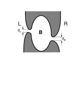
FIG. 4.: Schematic view of the ballistic cavity “B” between two reservoirs “L” and “R”.

Let us consider the system consisting of three cavities, see Fig. 4, connected by channels. The size of the central cavity (“B” in Fig. 4) is much smaller than that of the outer cavities (“L” and “R” in Fig. 4) which act as reservoirs. The conductance of the system is controlled by the channels so that their widths $d_{L,R}$ are much smaller than the characteristic size of the central cavity, $d_{L,R}\ll a$. We assume that the motion of an electron in the channel still can be described by the classical Liouville equation, which implies $d_{L,R}\gg\lambda_{F}$.

Because of the inequality $d_{L,R}\ll a$, the time it takes to establish the equilibrium distribution function in the cavity is much smaller than the escape time. (The equilibration time is of the order of the flying time of the electron across the cavity.) Under such conditions the classical escape times from the cavity through the left (right) channel $\tau_{L(R)}$ are given by

$$\!\!\frac{1}{\tau_{L(R)}}\!=\!\frac{1}{{\cal A}_{B}}\!\int\!\!\frac{dn}{2\pi}\!\!\int\!\!\theta\left({\bf n}\!\cdot\!d\mbox{\boldmath$\ell$}\right)v_{L(R)}{\bf n}\!\cdot\!d\mbox{\boldmath$\ell^{L(R)}$}\!=\!\frac{d_{L(R)}v_{L(R)}}{2{\cal A}_{B}},$$ (175)

where ${\cal A}_{B}$ is the area of the cavity, the linear integration is performed along the narrowest cross-section of the corresponding channel, $d\mbox{\boldmath$\ell$}^{L(R)}$ is directed outside the cavity “B” normal to the integration line, and $v_{L(R)}$ are the Fermi velocities in the contacts. Equation (175) corresponds to the classical Sharvin formula[22] for 2D case and the escape times are related to the classical conductance of a single channel $g_{L(R)}$ by

$$g_{L(R)}=\frac{se^{2}\nu{\cal A}_{B}}{\tau_{L(R)}}.$$ (176)

If the external bias $eV(t)$ is applied to, say, left reservoir, (the right reservoir is maintained at zero bias), the electric current $I$ from the left to the right reservoir appears. This current is linear in the applied bias:

$$\displaystyle{I(t)\equiv-\dot{Q}_{L}(t)=\int_{-\infty}^{t}dt^{\prime}g(t-t^{\prime})V(t^{\prime}),}$$ (177)

$$\displaystyle{g(t)=\int\frac{d\omega}{2\pi}e^{-i\omega t}g(\omega),}$$ (178)

where ${Q}_{L}$ is the charge of the left reservoir. Relation Eq. (178) defines the conductance of the system $g(\omega)$. Performing actual calculations in Eq. (178), one has to take into account the condition of the electroneutrality in the cavity “B”, $\dot{Q}_{B}=0$. The electroneutrality requirement is valid at times larger the characteristic time of the charge relaxation. This time $\tau_{c}$ can be estimated as $\tau_{c}\simeq C_{B}/({\rm max}\ g_{L,R})$, where $C_{B}$ is the capacitance of the cavity. Using estimate $C_{B}\sim a$ and formulas (175), (176), we find $\tau_{c}\simeq\tau_{fl}a_{B}/({\rm max}\ d_{L,R})$, where $\tau_{fl}=a/v_{F}$ is the flying time of the electron across the cavity, and $a_{B}$ is the screening radius in 2D electron systems. For wide channels $d_{L,R}\gg\lambda_{F}\simeq a_{B}$, we have $\tau_{c}\ll\tau_{fl}$. We are interested in the dynamics of the system at time much larger than the flying time and, therefore, we can assume that the electroneutrality holds.

Then, the standard linear response calculations enable us to relate the conductance $g$ to the diffuson ${\cal D}$ defined in Sec. II. The charge response in $i$th cavity, $Q_{i}$ to the applied biases $V(t),V_{B}(t)=V,V_{B}e^{-i\omega t}$ can be expressed by means of the polarization operator as

$$Q_{i}=\!e^{2}\!\!\int\!\!d{\bf r}_{1}d{\bf r}_{2}\Pi\left(\omega;{\bf r}_{1},{\bf r}_{2}\right)\!\theta_{i}({\bf r_{1}})\!\left[V\theta_{L}({\bf r_{2}})+V_{B}\theta_{B}({\bf r_{2}})\right],$$ (179)

where function $\theta_{i}({\bf R})$ equals to unity if vector ${\bf R}$ lies in the $i$th region ($i=L,R,B$) and equals to zero otherwise. The potential $V_{B}$ is to be found self-consistently from the electroneutrality requirement. Substituting Eq. (29) into Eq. (179) and making use of Eqs. (32), and (44), we obtain with the help of definition (178)

$$\displaystyle{g(\omega)=se^{2}\nu\left\{-i\omega{\cal A}_{L}+\omega^{2}\left[{\cal D}_{LL}(\omega)+{\cal D}_{LB}(\omega)\frac{V_{B}}{V}\right]\right\};}$$ (180)

$$\displaystyle{{\cal D}_{ij}(\omega)\equiv\int\frac{d{\bf n_{1}}d{\bf n_{2}}d{\bf R_{1}}d{\bf R_{2}}}{\left(2\pi\right)^{2}}\theta_{i}({\bf R_{1}})\theta_{j}({\bf R_{2}})}$$ (181)

$$\displaystyle{\hskip 85.35826pt\times{\cal D}_{\epsilon_{F}}(\omega;{\bf n_{1}},{\bf R_{1}};{\bf n_{2}},{\bf R_{2}}),}$$ (182)

where ${\cal A}_{i}$ is the area of the corresponding region ($i=L,R,B$).

The electroneutrality condition, $Q_{B}=0$, gives us the equation for the potential of the cavity $V_{B}$. Using Eq. (179) for $i=B$, we find with the help of Eqs. (29), (32) and (44)

$$i\omega{\cal D}_{LB}(\omega)V+\left[{\cal A}_{B}+i\omega{\cal D}_{BB}(\omega)\right]V_{B}=0.$$ (183)

A Classical conductance

Let us first calculate the classical conductance $g_{cl}$ of the system. We consider the frequencies $\omega$, much smaller than the flying time of the electron in a cavity. Assuming that the motion in the cavity is ergodic and the areas of the reservoirs are large, ${\cal A}_{L(R)}/{\cal A}_{B}\gg\omega\tau_{L(R)}$, we obtain that the diffuson changes only within the channels. For ${\cal D}_{ij}$ from Eq. (182) we find

$$\displaystyle{{\cal D}_{BB}^{0}(\omega)=\frac{{\cal A}_{B}}{-i\omega+\frac{1}{\tau_{B}}},\quad\frac{1}{\tau_{B}}=\frac{1}{\tau_{L}}+\frac{1}{\tau_{R}}}$$ (185)

$$\displaystyle{{\cal D}_{jj}^{0}(\omega)=\frac{{\cal A}_{j}}{-i\omega}+\frac{{\cal A}_{B}}{\tau_{j}\omega^{2}}-\frac{{D}_{BB}^{0}}{\left(\tau_{j}\omega\right)^{2}},\quad j=L,R};$$ (186)

$$\displaystyle{{\cal D}_{jB}^{0}(\omega)={\cal D}_{Bj}^{0}(\omega)=\frac{{\cal D}_{BB}^{0}(\omega)}{-i\omega\tau_{j}},\quad j=L,R};$$ (187)

$$\displaystyle{{\cal D}_{LR}^{0}(\omega)={\cal D}_{RL}^{0}(\omega)=-\frac{{\cal D}_{BB}^{0}(\omega)}{\omega^{2}\tau_{L}\tau_{R}}.}$$ (188)

Equation (185) describes the exponentially decaying in time probability to find the electron in the cavity “B” if it started in this cavity. First term in Eq. (186) corresponds to the classical correlator of the $j$th reservoir disconnected from the cavity, the second term describes the finite probability for the electron to enter cavity “B” from $j$th reservoir, and the third term corresponds to the process in which an electron from $j$th reservoir visits the cavity once and then comes back. Equation (187) gives the probability for the electron to appear in the $j$th reservoir starting from the cavity. Finally, Eq. (188) is the probability for an electron to get from the left to the right reservoir.

Substituting Eqs. (VI A) into Eq. (183), we find that the bias of the cavity $V_{B}$ does not depend on frequency, $V_{B}=g_{L}/\left(g_{L}+g_{R}\right)$. Then, by substitution Eqs. (VI A) into Eqs. (182), we obtain with the help of Eq. (176)

$$g_{cl}=\frac{g_{L}g_{R}}{g_{L}+g_{R}}$$ (189)

in agreement with the Kirchhoff law. It is worth mentioning that the result (189) at $\omega=0$ can be obtained without requirement of the electroneutrality.

B Weak localization correction

In order to calculate the weak localization correction to the conductance $\Delta g(\omega)$ we have to find the correction to the classical correlator $\Delta{\cal D}$ and then use Eq. (182) and (183). For such calculation, it is most convenient to use Eq. (77). Our strategy will be analogous to the one we used in Sec. IV for the calculation of the correction to the conductivity.

Integrating both sides of Eq. (77) over the coordinates $1$ and $2$ within the regions specified by $\theta$-functions in Eq. (182) and using obvious relation ${\cal D}(1,2)={\cal D}(\bar{2},\bar{1})$, we obtain

$$\Delta{\cal D}_{ij}=\Delta{\cal D}_{ji}^{(1)}+\Delta{\cal D}_{ji}^{(2)},$$ (190)

$$\Delta{\cal D}_{ji}^{(1)}=\int d1\left[\raisebox{0.0pt}[5.69054pt][5.69054pt]{${\cal D}^{0}_{j}(1)\theta_{i}({\bf R}_{1})+{\cal D}^{0}_{i}(\bar{1})\theta_{j}({\bf R}_{1})$}\right]\frac{{\cal C}^{0}(1,\bar{1})}{2\pi\nu},$$ (191)

$$\Delta{\cal D}_{ji}^{(2)}=\int d1{\cal D}^{0}_{i}(1){\cal D}^{0}_{j}(1)\left[2i\omega-\hat{L}_{1}+\frac{1}{\tau_{q}}\frac{\partial^{2}}{\partial\phi^{2}_{1}}\right]\frac{{\cal C}^{0}(1,\bar{1})}{2\pi\nu},$$ (192)

where

$${\cal D}^{0}_{i}(1)\equiv\int d2\theta_{i}({\bf R}_{2}){\cal D}^{0}(2,1).$$ (193)

Here, we use the short hand notation $l\equiv({\bf n}_{l},{\bf R}_{l})$, integration over the phase space on the energy shell is defined as $dl\equiv d{\bf n}_{l}d{\bf R}_{l}/2\pi$, and the time reversed coordinate $\bar{l}$ is given by $\bar{l}\equiv(-{\bf n}_{l},{\bf R}_{l})$.

It is noteworthy, that the quantum correction $\Delta{\cal D}_{ij}$ satisfy the charge conservation condition

$$\sum_{j=L,R,B}\Delta{\cal D}_{ij}=0,\quad i=L,R,B$$ (194)

which can be easily proven with the help of the relation $\sum_{i}{\cal D}^{0}_{i}(1)=\frac{1}{-i\omega}$ and Eq. (75). Equation (194) enables us to consider only non-diagonal elements of $\Delta{\cal D}_{ij}$ which is technically easier.

Analogous to the discussion in Sec.IV, we assume that the Cooperon part of the expression can be calculated independently of the diffuson part. This is because the classical trajectories corresponding to these quantities traverse essentially the different regions of the phase space.

First, we use this assumption to evaluate contribution $\Delta{\cal D}^{(1)}$ from Eq. (190). We notice that the classical trajectory can close only inside the cavity. Therefore, the Cooperon ${\cal C}(1,\bar{1})$ also exists only inside the cavity “B”. For the calculation of the diffuson, we notice that at times much larger than the flying time across the cavity $\tau_{fl}$ the position of the electron and its momentum is randomized. It suggests to use the approximation

$${\cal D}^{0}_{i}(1)\approx\frac{1}{{\cal A}_{B}}\int d1{\cal D}^{0}_{i}(1)\theta_{B}({\bf R}_{1})=\frac{{\cal D}^{0}_{iB}}{{\cal A}_{B}},$$ (195)

if vector $R_{1}$ lies inside the cavity. Here, function ${\cal D}^{0}_{ij}$ is defined in Eq. (VI A). Using Eq. (195), we obtain

$$\Delta{\cal D}_{ji}^{(1)}=\left[\raisebox{0.0pt}[5.69054pt][5.69054pt]{${\cal D}^{0}_{jB}\delta_{iB}+{\cal D}^{0}_{iB}\delta_{jB}$}\right]\frac{\langle{\cal C}^{0}(1,\bar{1})\rangle}{2\pi\nu}$$ (196)

where the average inside the cavity is defined as

$\displaystyle\langle\dots\rangle=\frac{1}{{\cal A}_{B}}\int d1\theta_{B}({\bf R}_{1})\dots\ .$Let us turn to the calculation of the contribution $\Delta{\cal D}^{(2)}_{ij}$. As we already saw in Secs. II and IV, two diffusons can not be averaged independently, because motion of their ends are governed by the same potential during period $t_{E}\gg\tau_{tr}$. On the other hand, the randomization of the motion of the center of mass occurs during in a time interval of the order $\tau_{fl}$. Therefore, we can approximate

$${\cal D}^{0}_{i}(1){\cal D}^{0}_{j}(1)\approx\theta_{B}({\bf R}_{1})\langle{\cal D}^{0}_{i}(1){\cal D}^{0}_{j}(1)\rangle.$$ (197)

Expression (197) is written in the lowest order in small parameter ${\cal A}_{B}/{\cal A}_{L,R}$, and we exclude from our consideration cases $i=j=L,R$. In the latter cases, there are also non-vanishing contributions in Eq. (197) corresponding to the coordinate ${\bf R}_{1}$ in the reservoirs $L$ or $R$. This would require more careful investigation of the behavior of the diffuson in the channels. We, however, simply bypass this difficulty by utilizing identity (194) for the calculation of the diagonal elements $\Delta{\cal D}_{LL}$ and $\Delta{\cal D}_{RR}$. Using the approximation (197), we find

$$\Delta{\cal D}_{ji}^{(2)}=\langle{\cal D}^{0}_{i}(1){\cal D}^{0}_{j}(1)\rangle\!\int\!d1\ \theta_{B}({\bf R}_{1})\left[\raisebox{0.0pt}[5.69054pt][5.69054pt]{$2i\omega-\hat{L}_{1}$}\right]\frac{{\cal C}^{0}(1,\bar{1})}{2\pi\nu}.$$ (198)

Liouvillean operator $\hat{L}_{1}$ in the second term of the RHS of Eq. (198) is the total derivative along a classical trajectory and, therefore, it can be reduced to the linear integrals across the channels

$$\int\!d1\ \theta_{B}({\bf R}_{1})\hat{L}_{1}{\cal C}^{0}(1,\bar{1})=$$ (199)

$$\hskip 48.36958pt\int\frac{dn_{1}}{2\pi}\left(\int\!{\bf n}_{1}\cdot d\mbox{\boldmath$\ell^{L}_{1}$}+\!\!\int\!{\bf n}_{1}\cdot d\mbox{\boldmath$\ell^{R}_{1}$}\right)v_{F}{\cal C}^{0}(1,\bar{1})$$ (200)

where the linear integration is defined similar to that in Eq. (175). Then, we notice that a classical trajectory can close only inside the cavity. Therefore, only the Cooperons with the initial momentum directed inside the cavity exist. Assuming that the randomization of the momentum direction occurs only inside the cavity and considering the times much larger than the flying time, we conclude that the Cooperon in the contact vanishes if its moment ${\bf n}_{1}$ directed inside the cavity and for the moment directed outside the cavity Cooperon coincides with its value inside the cavity, ${\cal C}(1,\bar{1})=\theta\left({\bf n}_{1}\cdot d{\bf\ell}_{L(R)}\right)\langle{\cal C}(1,\bar{1})\rangle$ for the coordinate $R_{1}$ located in the left or right channel respectively. This enables us to reduce Eq. (199) to the simple form

$$\int\!d1\ \theta_{B}({\bf R}_{1})\hat{L}_{1}{\cal C}^{0}(1,\bar{1})=\frac{{\cal A}_{B}}{\tau_{B}}\langle{\cal C}(1,\bar{1})\rangle,$$ (201)

where the total escape time $\tau_{B}$ is defined in Eq. (185). Deriving Eq. (201), we use the definition of the escape times (175). Arguments above are essentially equivalent to those in the derivation of the classical Sharvin conductance[22].

Combining formulas (196), (198), (201) and (190), we obtain

$$\Delta{\cal D}_{ji}=\frac{\langle{\cal C}^{0}(1,\bar{1})\rangle}{2\pi\nu}\left[\raisebox{0.0pt}[8.53581pt][8.53581pt]{${\cal D}^{0}_{jB}\delta_{iB}+{\cal D}^{0}_{iB}\delta_{jB}+$}\right.$$ (202)

$$\quad\quad\quad\quad\left.\left(2i\omega-\frac{1}{\tau_{B}}\right){\cal A}_{B}\langle{\cal D}^{0}_{i}(1){\cal D}^{0}_{j}(1)\rangle\right].$$ (203)

We reiterate that Eq. (202) is not applicable for the case of $i=j=L,R$. In order to find the diagonal elements $\Delta{\cal D}_{LL}$ and $\Delta{\cal D}_{RR}$, one has to use the identity (194).

The calculation of the corresponding averages $\langle{\cal C}^{0}(1,\bar{1})\rangle$ and $\langle{\cal D}^{0}_{i}(1){\cal D}^{0}_{j}(1)\rangle$ is performed along the lines of the derivations in Sec. IV. In the calculation of the Cooperon the only change is in the expression (83) for the Cooperon outside the Lyapunov region

$$C(\phi,\rho)=\frac{1}{{\cal A}_{B}\left(-i\omega+\frac{1}{\tau_{B}}\right)},$$ (204)

which is analogous to Eq. (185) The solution for the Cooperon in the Lyapunov region is analogous to one presented in Secs. IV A and IV E. The calculation of function $w$ may be performed for the cavity disconnected from the reservoirs, provided that the condition $t_{E}\ll\tau_{B}$ holds. As the result we obtain

$$\langle{\cal C}(1,\bar{1})\rangle=\frac{w(\omega,0,0)}{{\cal A}_{B}\left(-i\omega+\frac{1}{\tau_{B}}\right)}.$$ (205)

In the calculation of the product of two diffusons $\langle{\cal D}^{0}_{i}(1){\cal D}^{0}_{j}(1)\rangle$ the change should be made in Eq. (113). The reason for this is that the integration over ${\bf R},{\bf n}$ for the reducing Eq. (108) to Eq. (111) is performed now only inside the cavity. As a result, one more term

$\displaystyle\int\frac{d{\bf n}d{\bf R}}{2\pi}\theta_{B}({\bf R})\hat{L}_{c}{\cal M}_{1}\left(1,2;{\bf n},{\bf R};\phi,\rho\right)\approx\frac{{M}_{1}\left(1,2;\phi,\rho\right)}{\tau_{B}}$[cf. with the derivation of Eq. (201)] has to be added to the LHS of Eq. (111). Equation (113), then, acquires the form

$\displaystyle M_{1}(1,2;\rho,\phi)=\frac{\langle{\cal D}^{0}\!\left(\bar{1};2\right)\rangle\!+\!\langle{\cal D}^{0}\!\left(1;\bar{2}\right)\rangle}{-2i\omega+\frac{1}{\tau_{B}}},$and we obtain instead of Eq. (119)

$${\cal A}_{B}\langle{\cal D}^{0}_{i}(1){\cal D}^{0}_{j}(1)\rangle\!=\!w(\omega;0,0)\frac{{\cal D}^{0}_{iB}{\cal D}^{0}_{jB}}{{\cal A}_{B}}+$$ (206)

$$\hskip 34.14322pt\frac{1-w(\omega;0,0)}{-2i\omega+\frac{1}{\tau_{B}}}\left[{\cal D}^{0}_{iB}\delta_{jB}+{\cal D}^{0}_{jB}\delta_{iB},\right],$$ (207)

where functions ${\cal D}^{0}_{iB}$ are given by Eqs. (185) and (187). Result (207) is not applicable for $i=j=L,R$ cases. Deriving Eq. (207), we used Eq. (195) for the average of the single diffuson $\langle{\cal D}^{0}_{i}(1)\rangle$.

Substituting Eqs. (205) and (207) into Eq. (202), we obtain with the help of Eqs. (VI A) and (123)

$$\Delta{\cal D}_{BB}\left(\omega\right)=\frac{\Gamma(\omega)}{2\pi\nu}\frac{\frac{1}{\tau_{B}}}{\left(-i\omega+\frac{1}{\tau_{B}}\right)^{3}};$$ (209)

$$\Delta{\cal D}_{jB}=\Delta{\cal D}_{Bj}=-\frac{\tau_{B}}{\tau_{j}}\Delta{\cal D}_{BB},\quad j=L,R;$$ (210)

$$\Delta{\cal D}_{LR}=\frac{1-2i\omega{\tau_{B}}}{\omega^{2}\tau_{L}\tau_{R}}\Delta{\cal D}_{BB}\left(\omega\right).$$ (211)

Corrections $\Delta{\cal D}_{jj}$ for $j=L,R$ are found with help of Eq. (194) and they are given by

$$\Delta{\cal D}_{jj}=\left(\frac{2i\omega{\tau_{B}}-1}{\omega^{2}\tau_{L}\tau_{R}}+\frac{\tau_{B}}{\tau_{j}}\right)\Delta{\cal D}_{BB}.$$ (212)

Substituting Eqs. (209) and (211) into Eq. (183), we observe that the voltage in the cavity $V_{B}$ does not acquire any quantum corrections, $V_{B}=Vg_{L}/\left(g_{R}+g_{L}\right)$. Finally, substituting Eqs. (VI B) into Eq. (182) and using Eq. (176), we obtain the final result for the frequency dependent weak localization correction to the conductance of the ballistic cavity

$$\Delta g(\omega)=-\frac{se^{2}}{2\pi\hbar}\frac{g_{L}g_{R}}{\left(g_{L}+g_{R}\right)^{2}}\left[\frac{\Gamma(\omega)}{1-i\omega\tau_{B}}\right],$$ (213)

where the total escape time $\tau_{B}$ is defined in Eq. (185) We emphasize that Eq. (213) at zero frequency can be obtained without electroneutrality requirement.

Equation (213) is the main result of this section. At $\omega=0$, this result agrees with the findings of Ref. [[10]] in the limit of large number of quantum channels in the contact. We are aware of neither any calculation at finite frequency nor of a description of the role of the Ehrenfest time in the conductance of the ballistic cavities. The renormalization function $\Gamma(\omega)$ in Eqs. (213) describes the effect of the Lyapunov region on the weak localization and it is given by Eqs. (2) and (3). Analytic calculation of the Lyapunov exponents $\lambda,\lambda_{2}\simeq\tau_{fl}^{-1}$ for the ballistic cavity is a separate problem and it will not be done in this paper. It is assumed in Eq. (213), that the condition $t_{E}\ll\tau_{B}$ holds. The result for the opposite limit, (which corresponds to the exponentially small Planck constant), is obtained by substitution $\Gamma(\omega)\to\Gamma(\omega+i/\tau_{B})$ in Eq. (213) and the weak localization correction turns out to be suppressed by the factor $\exp\left(-2t_{E}/\tau_{B}\right)$.

The finite phase relaxation time $\tau_{\varphi}$ is taken into account by substitution $\omega\to\omega+i/\tau_{\varphi}$ in Eq. (205). At $\tau_{\varphi}\gg t_{E}$, the result for $dc$- conductance agrees with the result of Ref. [[23]]. We obtained for $\omega=0$

$$\Delta g=-\frac{se^{2}}{2\pi\hbar}\frac{{g_{L}g_{R}}}{\left(g_{L}+g_{R}\right)^{2}}\frac{\tau_{i}}{\tau_{B}}\times$$ (214)

$$\hskip 56.9055pt\exp\!\left[-\frac{t_{E}}{\tau_{i}}\!\left(1\!-\!\frac{\lambda_{2}}{\lambda^{2}{\tau_{i}}}\right)-\frac{t_{E}}{\tau_{B}}\!\left(1\!-\!\frac{\lambda_{2}}{\lambda^{2}{\tau_{B}}}\!\right)\right],$$ (215)

where $\tau_{i}$ is the time it takes for an electron to be scattered inelastically or to escape the cavity,

$\displaystyle\frac{1}{\tau_{i}}=\frac{1}{\tau_{B}}+\frac{1}{\tau_{i}}.$Usually, the Ehrenfest time $t_{E}$ is much smaller than the escape time $\tau_{B}$. In this case, one can immediately see the dramatic crossover at the temperature dependence (usually $\tau_{\varphi}$ is a power function of temperature, see Ref. [[13]]). If at $\tau_{\varphi}\gg t_{E}$, the dependence on temperature is a power law, with the increase of the temperature the change to the exponential drop occurs. Thus, the study of the crossover in the temperature or frequency dependence of the ballistic cavities may provide the information about the values and the distribution of the Lyapunov exponents in the cavity.

VII Conclusion

In this paper we developed a theory for the weak localization (WL) correction in a quantum chaotic system, i.e. in a system with the characteristic spatial scale of the static potential, $a$, being much larger than the Fermi wavelength, $\lambda_{F}$. We showed that for the quantum chaos, new frequency domain appears, $t_{E}^{-1}\ll\omega\ll\tau_{tr}^{-1}$, [$t_{E}$ is the Ehrenfest time, see Eq. (3)] where the classical dynamics is still governed by the diffusion equation, but the WL correction deviates from the universal law. For the first time, we were able to investigate frequency dependence of the WL correction at such frequencies, see Eqs. (1) and (2), and to find out how the fundamental characteristic of the classical chaos appears in the quantum correction. At lower frequencies, $\omega\ll t_{E}^{-1}$, we proved the universality of the weak localization correction for the disorder potential of an arbitrary strength and spatial size.

These results may be experimentally checked by studying the frequency or temperature (via $\tau_{\varphi}$) dependence of the weak localization correction (e.g. negative magnetoresistance). Indeed, at the low-frequency or temperature, the conventional dependence should be observed. This dependence is rather weak (logarithmical for large samples and a power law for the ballistic cavities). With the increase of the frequency or temperature, the dependence becomes exponential; such a crossover may be used to find the Ehrenfest time, $t_{E}$ and thus extract the value of the Lyapunov exponent. The parameters of the ballistic cavities studied in Ref. [[8]] are $a\simeq 1\mu m,\ \lambda_{F}\simeq 400\AA$, so that $\ln(a/\lambda_{F})\simeq 3$. We believe, however, that the size of the ballistic cavities may be raised up to the mean free path $\simeq 17\mu m$; Ehrenfest time in this case would be appreciably larger than the flying time, $\ln(a/\lambda_{F})\simeq 6$, and the characteristic frequency $\omega=t_{E}^{-1}$ for this case can be estimated as $\omega\simeq 5\times 10^{9}s^{-1}$. Measurements of frequency dependence of the WL correction in quantum disorder regime were performed in Ref. [[24]] at frequency as high as $16.5\ {\rm GHz}$. Thus, the measurement of the Ehrenfest time in the ballistic cavities does not seem to be unrealistic.

We expect that the effects associated with the Ehrenfest time may be found also in optics. They may be observed, e.g. in the dependence of the enhanced backscattering on frequency of the amplitude modulation $\omega$, This dependence should be still given by our function $\Gamma(\omega)$ with $\lambda_{F}$ being replaced with the light wavelength.

We showed that the description of the intermediate region $t_{E}^{-1}\ll\omega\ll\tau_{tr}^{-1}$ can be reduced to the solution of the purely classical equation of motion, however, the averaging leading to the Boltzmann equation is not possible because the initial and final phase cells of the relevant classical correlator (Cooperon) are related by the time inversion. Therefore, the initial and finite segments of the corresponding classical trajectory are strongly correlated and their relative motion is described by the Lyapunov exponent and not by the diffusion equation. We took this correlation into account, showed that it is described by the log-normal distribution function and related the Ehrenfest time to the parameters of this function.

Because the description by the Boltzmann equation was not possible, we derived the lowest order quantum correction to the classical correlator in terms of the solution of the Liouville equation, smeared by the small angle diffraction, see Eq. (74). The derivation was based on the equations of motion for the exact Green functions and did not imply averaging over the realization of the potential.

Closing the paper, we would like to discuss its relation to the other works and to make few remarks concerning how the Ehrenfest time appears in the level statistics.

First, we notice that, though quite popular in the classical mechanics and hydrodynamics, the Lyapunov exponent very rarely enters in the expressions for observable quantities in the solid state physics, see Ref. [[15]]. The possibility to observe the intermediate frequency region $t_{E}^{-1}\ll\omega\ll\tau_{tr}$ appeared only recently with the technological advances in the preparing of the ballistic cavities and that is why the region has not been studied systematically as of yet. Let us mention that the importance of the Ehrenfest time in the semiclassical approximation was noticed already in Ref. [[15]] where it was shown that the method of quasiclassical trajectories in the theory of superconductivity[16] fails to describe some non-trivial effect at times larger than $t_{E}$ which was calculated for the dilute scatterers. The term “Ehrenfest time” for the quantity (3) was first introduced in Ref. [[25]] The relevance of $t_{E}$ in the theory of weak localization was emphasized by Argaman[11], however, he focused only on times much larger than the Ehrenfest time.

The universality of weak localization correction at small frequencies was known for the case of weak quantum impurities[4] and for the ballistic cavities[10]. We are not aware of any proof of the universality for the disorder potential of arbitrary strength and spatial scale.

The description of the quantum corrections in terms of the nonaveraged solutions of the Liouville equation was developed in by Muzykantskii and Khmelnitskii[26] and more recently by Andreev et. al.[27], who suggested the effective supresymmetric[28] action in the ballistic regime. In Ref.[[27]], the supersymmetric action was written in terms of the Perron-Frobenius operator which differs from the first order Liouville operator by the regularizator of the second order. This regularizator is similar to the angular diffusion term, $\propto 1/\tau_{q}$ in Eqs. (III B). The authors mentioned that all the physical results can be obtained if the limit of vanishing regularizator is taken in the very end of the calculation. Our finding indicate that the time it takes for the quantum correction to reach its universal value is $\propto\ln\left(\tau_{q}\right)$. Thus, at any finite frequency, the limit $\tau_{q}\to\infty$ can not be taken and the regularizator in the supersymmetric action should be assigned its physical value, see Eq. (71).

In principle, our formula for the weak localization correction (74) can be derived using the supersymmetry technique. However, our approach seems to be technically easier and more physically tractable for the calculation of the first order weak localization correction. We believe that the supersymmetry may serve as a powerful tool for the investigation of the effect of the Ehrenfest time on the higher order corrections and on the level statistics.

It is generally accepted that the level statistics at low energies is described by the Wigner-Dyson distribution[29]. For the small disordered particle it was first proven by Efetov[28] and for the ballistic cavities by Andreev et. al.[27]. For the quantum disorder, Altshuler and Shklovskii[30] showed that the universal Wigner-Dyson statistics breaks down at the Thouless energy. For the ballistic cavities the universal statistics is believed to be valid up to the energies of the order of the inverse flying time $\tau_{fl}$, at smaller energies $s$ the corresponding corrections are small as $s\tau_{fl}$. We, however, anticipate deviations at the parametrically smaller energies of the order of $t_{E}^{-1}$, and the corrections of the order of $st_{E}$ at energies $s\ll t_{E}^{-1}$.

Let us consider for concreteness the correlator of the density of states ${\cal R}(s)=\langle\rho(\epsilon)\rho(\epsilon+s)\rangle-\langle\rho(\epsilon)\rangle^{2}$, where $\rho(\epsilon)=Tr\delta\left(\epsilon-\hat{H}\right)$. For the orthogonal gaussian ensemble the random matrix theory yields[29] ${\cal R}(s)=-\left(\pi s\right)^{-2}+\left(1+\cos^{2}\pi s\right)/\left(\pi s\right)^{-4}+\dots$, where $s\gg 1$ is measured in units of mean level spacing. We expect, that the first term in this expression is not affected by the presence of the Lyapunov region, whereas the following terms are. In the supersymmetric approach[28] this follows from the fact that the first term arises from non interacting diffuson modes whereas all the others come from the interaction of these modes. Such interaction is analogous to the one giving rise to the weak localization which was shown to have the frequency dispersion described by the renormalization function $\Gamma(\omega)$, see Eq. (2). We believe that the same renormalization factor will appear in all the effects associated with the coupling of the diffuson-Cooperon modes.

A Lyapunov exponent for the weak scatterers

We consider explicitly the case where the potential $U$ in Eq. (126) is weak and its distribution function is Gaussian. For the sake of simplicity we neglect the angular diffusion due to the quantum impurities in the Lyapunov region, because this diffusion does not affect values of $\lambda,\ \lambda_{2}$, see Sec. IV E. In this case it is more convenient not to follow the general procedure outlined in Sec. (IV E), but to make use of the small parameter $a/\l_{tr}$ first. Considering the disorder potential in the second order of the perturbation theory, we obtain for independent on ${\bf R},{\bf n}$ part of the function $W_{\perp}$:

$$\left[\frac{\partial}{\partial t}-v_{F}\phi\frac{\partial}{\partial\rho}-\frac{2}{\tau_{tr}}{\cal E}(\rho)\frac{\partial^{2}}{\partial\phi^{2}}\right]W_{\perp}=0,$$ (A1)

where the transport life time is given by

$$\frac{1}{\tau_{tr}}=\frac{1}{4\epsilon_{F}p_{F}}\int_{-\infty}^{\infty}dx\langle\partial_{y}U(x,0)\partial_{y}U(0,0)\rangle,$$ (A2)

and the dimensionless function ${\cal E}$ is defined as

$${\cal E}(\rho)=1-\frac{\int_{-\infty}^{\infty}dx\langle\partial_{y}U(x,\rho)\partial_{y}U(0,0)\rangle}{\int_{-\infty}^{\infty}dx\langle\partial_{y}U(x,0)\partial_{y}U(0,0)\rangle}.$$ (A3)

In Eq. (A1), we assumed $\phi\ll 1$ only and lifted the other assumption of Eq. (126) $\rho\ll a$. If $\rho\ll a$, we expand ${\cal E}$ in Taylor series, ${\cal E}(\rho)\approx\rho^{2}/2a^{2}$, which rigorously defines length $a$ in this case, and we arrive to the equation describing the Lyapunov region for the weak disorder potential

$$\left[\frac{\partial}{\partial t}-v_{F}\phi\frac{\partial}{\partial\rho}-\frac{\rho^{2}}{\tau_{tr}a^{2}}\frac{\partial^{2}}{\partial\phi^{2}}\right]W_{\perp}=0.$$ (A4)

It is worth noticing, that our approach is equivalent to one involving the multiplication of the vector $(\rho,\phi)$ by a Monodromy matrix after each scattering event. Equation (A4) is valid because each Monodromy matrix defined on a time of the order $a/v_{F}$ is close to unit matrix. Otherwise, the last term in the brackets in Eq. (A4) becomes an integral operator.

After introduction of new variables

$$z=\ln\frac{a}{\rho},\quad y=\frac{a\phi}{\rho}\left(\frac{l_{tr}}{a}\right)^{1/3}\!\!\!,\quad\tau=\frac{t}{\tau_{tr}}\left(\frac{l_{tr}}{a}\right)^{2/3}\!\!\!,$$ (A5)

equation (A4) acquires a simple form

$$\left[\frac{\partial}{\partial\tau}-y\frac{\partial}{\partial z}+y^{2}\frac{\partial}{\partial y}-\frac{\partial^{2}}{\partial y^{2}}\right]W_{\perp}=0.$$ (A6)

We are interested in the case when function $W_{\perp}$ changes slowly as the function of $z$. Corresponding gradient is small, and we can employ the procedure similar to the reducing the Boltzmann equation to the diffusion equation. Let us represent function $W_{\perp}$ as

$$W_{\perp}(\tau;z,y)=W_{\perp}^{0}(\tau;z)+W^{1}(\tau;z,y),\quad W_{1}\ll W_{\perp}.$$ (A7)

Substituting Eq. (A7) into Eq. (A6), multiplying the result by function $g(y)$:

$$\left[\frac{d}{dy}y^{2}+\frac{d^{2}}{dy^{2}}\right]g(y)=0,\quad\int dyg(y)=1.$$ (A8)

and integrating over $y$ we obtain

$$\left[\frac{\partial}{\partial\tau}-\beta\frac{\partial}{\partial z}\right]W_{\perp}^{0}-\frac{\partial}{\partial z}\!\int\!dy\left[\left(y-\beta\right)g(y)W^{1}(y)\right]=0,$$ (A9)

where the numerical coefficient $\beta$ is given by

$$\beta=\int dy\ yg(y)$$ (A10)

and function $W^{1}$ can be written as

$$W^{1}=h(y)\frac{\partial W_{\perp}^{0}(\tau;z)}{\partial z},\ \left[y^{2}\frac{d}{dy}-\frac{d^{2}}{dy^{2}}\right]h(y)=y-\beta.$$ (A11)

Shift of $W^{1}$ by an arbitrary constant does not affect the results, see Eqs. (A13) and (A10). Substituting Eq. (A11) into Eq. (A9), we obtain in accordance with general formula (149)

$$\left[\frac{\partial}{\partial\tau}-\beta\frac{\partial}{\partial z}-\beta_{2}\frac{\partial^{2}}{\partial z^{2}}\right]W_{\perp}^{0}(\tau;z)=0,$$ (A12)

where the numerical coefficient $\beta_{2}$ is given by

$$\beta_{2}=\int dy\ \left(y-\beta\right)g(y)h(y).$$ (A13)

Comparing Eqs. (A12) and (A5) with Eq. (149), we find for Lyapunov exponent $\lambda$ and its deviation $\lambda_{2}$

$$\lambda=\frac{\beta}{\tau_{tr}}\left(\frac{l_{tr}}{a}\right)^{2/3},\quad\lambda_{2}=\frac{2\beta_{2}}{\tau_{tr}}\left(\frac{l_{tr}}{a}\right)^{2/3}.$$ (A14)

Simple calculation of the numeral coefficients $\beta,\beta_{2}$ is carried out with the help of Eqs. (A10), (A8), (A13) and (A11) with the final result

$$\displaystyle{\beta=\frac{\int_{-\infty}^{\infty}dy\ e^{-y^{3}/3}y\int_{-\infty}^{y}dy_{1}\ e^{y^{3}_{1}/3}}{\int_{-\infty}^{\infty}dy\ e^{-y^{3}/3}\int_{-\infty}^{y}dy_{1}\ e^{y^{3}_{1}/3}}\approx 0.365,}$$ (A15)

$$\displaystyle{\beta_{2}=\frac{\int_{-\infty}^{\infty}\!\!dy\left[e^{y^{3}/3}\!\!\int_{-\infty}^{y}\!\!dy_{1}e^{y^{3}_{1}/3}\!\!\left(\int^{\infty}_{y}\!dy_{2}(\beta\!-\!y_{2})e^{-y^{3}_{2}/3}\right)^{2}\right]}{\int_{-\infty}^{\infty}dy\ e^{-y^{3}/3}\int_{-\infty}^{y}dy_{1}\ e^{y^{3}_{1}/3}}}$$ (A16)

$$\displaystyle{\hskip 142.26378pt\approx 0.705.}$$ (A17)

In order to avoid any confusion, let us notice that the log-normal distribution function can not be used to find the averaged moments of the coordinates $\rho,\phi$ and it is sufficient only for the calculation of the low moments of the logarithm of the coordinates.

REFERENCES

- [1] Address after September 1, 1996: NEC Research Institute, Inc., Princeton, NJ 08540.
- [2] This result, strictly speaking, is applicable for the case of the strong scatterers where the transport and elastic mean free paths are of the same order. For the case of weak scatterers one should use instead of . Here is the Lyapunov exponent, see Appendix A.
- [3] E. Abrahams, P.W. Anderson, D.C. Licciardello, and T.V. Ramakrishnan, Phys. Rev. Lett, 42, 673 (1979);
- [4] L.P. Gorkov, A.I. Larkin, and D.E. Khmelnitskii, Pis’ma Zh. Eksp. Teor. Fiz., 30, 248 (1979) [JETP Lett. 30, 248 (1979)].
- [5] P.A. Lee and T.V. Ramakrishnan, Rev. Mod. Phys, 57 287 (1985); B.L. Altshuler, A.G. Aronov, D.E. Khmelnitskii, and A.I. Larkin, in Quantum Theory of Solids, edited by I.M. Lifshits, (MIR Publishers, 1983).
- [6] D. Weiss, K. Richter, A. Menschig, R. Bergmann, H. Schweizer, K. von Klitzing and G. Weimann, Phys. Rev. Lett, 70, 4118 (1993).
- [7] C.M. Marcus, A.J. Rimberg, R.M. Westervelt, P.F. Hopkins and G.A. Gossard, Phys. Rev. Lett, 69, 506 (1992).
- [8] A.M. Chang, H.U. Baranger, L.N. Pfeiffer, and K.W. West, Phys. Rev. Lett, 73, 2111 (1994).
- [9] H.U. Baranger, R.A. Jalabert, and A.D. Stone, Phys. Rev. Lett, 70, 3876 (1993).
- [10] H.U. Baranger and P.A. Mello, Phys. Rev. Lett. 73, 142 (1994); R. A. Jalabert, J.-L. Pichard, and C.W.J. Beenakker, Europhys. Lett. 27, 255 (1994).
- [11] N. Argaman, Phys. Rev. Lett., 75, 2750 (1995); Phys. Rev. B, 53, 7035 (1996).
- [12] The interaction effects analogous to those in the theory of QD[13] are beyond the scope of our paper.
- [13] B.L. Altshuler and A.G. Aronov, in Electron-Electron Interactions in Disordered Systems, edited by A.L. Efros and M. Pollak (North-Holland, Amsterdam, 1985).
- [14] N.S. Krylov, Works on the Foundations of Statistical Physics, (Princeton Unov. Press, Princeton, 1979).
- [15] A.I. Larkin and Yu.N. Ovchinnikov, Zh.Eksp.Teor.Fiz., 55, 2262 (1968) [Sov. Phys. JETP, 28, 1200 (1969)].
- [16] P.G. de Gennes, Rev. Mod. Phys. 36, 225 (1964); E.A. Shapoval, Zh.Eksp.Teor.Fiz., 49, 930 (1965) [Sov. Phys. JETP, 22, 647 (1966)].
- [17] A.I. Larkin and D.E. Khmelnitskii, Usp. Fiz. Nauk 136, 536 (1982); D. E. Khmelnitskii, Physica 126B, 235 (1984).
- [18] S. Chakravarty and A. Schmid, Phys. Rep. 140, 193 (1986).
- [19] Actually, these arguments give estimate rather than Eq. (3), however, the corresponding error in the definition of the Ehrenfest time is of the order of the . Because all the procedure is valid only for , keeping such terms in the exponent would be beyond the accuracy of the calculation.
- [20] B.L. Altshuler, D.E. Khmelnitskii, A.I. Larkin, and P.A. Lee, Phys. Rev. B 22, 5142 (1980); S. Hikami, A.I. Larkin and Y. Nagaoka, Progr. Teor. Phys. 63, 707 (1980).
- [21] A. Kawabata, J. Phys. Soc. Japan 49, 628 (1980); 53, 3540 (1984); M.I. Dyakonov, Sol. St. Comm, 92, 711 (1994).
- [22] Yu. V. Sharvin, Zh.Eksp.Teor.Fiz., 48, 984 (1965) [Sov. Phys. JETP, 21, 655 (1965)].
- [23] H.U. Baranger and P.A. Mello, Phys. Rev. B 51, 4703 (1995); P.W. Brouwer and C.W.J. Beenakker, ibid., 51, 7739 (1995).
- [24] G.U. Sumanasekera, B.D. Williams, D.V. Baxter, and J.P. Carini, Sol. St. Comm. 85, 941 (1993).
- [25] D.V. Chirikov, F.M. Izrailev, and D.L. Shepelyanskii, Sov. Sci. Rev. C2, 209 (1981).
- [26] B.A. Muzykantskii and D.E. Khmelnitskii, Pis’ma Zh. Eksp. Teor. Fiz., 62, 68 (1995) [JETP Letters, 62, 76 (1995)].
- [27] A.V. Andreev, O. Agam, B.D. Simons and B.L. Altshuler Phys. Rev. Lett. 76, 3947 (1996); (unpublished, cond/mat 9605204).
- [28] K. B. Efetov, Adv. Phys. 32, 53 (1983).
- [29] M.L. Mehta, Random Matrices, (Academic, New York, 1991).
- [30] B.L. Altshuler and B.I. Shklovskii, Zh.Eksp.Teor.Fiz., 91, 220 (1986) [Sov. Phys. JETP, 64, 127 (1986)].