Quantized Thermal Transport in the Fractional Quantum Hall Effect

Abstract

We analyze thermal transport in the fractional quantum Hall effect (FQHE), employing a Luttinger liquid model of edge states. Impurity mediated inter-channel scattering events are incorporated in a hydrodynamic description of heat and charge transport. The thermal Hall conductance, $K_{H}$, is shown to provide a new and universal characterization of the FQHE state, and reveals non-trivial information about the edge structure. The Lorenz ratio between thermal and electrical Hall conductances violates the free-electron Wiedemann-Franz law, and for some fractional states is predicted to be negative. We argue that thermal transport may provide a unique way to detect the presence of the elusive upstream propagating modes, predicted for fractions such as $\nu=2/3$ and $\nu=3/5$.

]

I Introduction

The connection between quantized electrical transport and the microscopic structure of edge states is of fundamental importance to the quantum Hall effect[1]. The Hall conductance is related to the additional edge current $J$ which flows when the chemical potential $\mu$ of the edge is raised,

$$G_{H}=e{\partial J\over{\partial\mu}}.$$ (1)

In the integer quantum Hall effect, the edge states consist of a single non-interacting electron mode for each full Landau level. Due to the cancellation between velocity and 1d density of states, the contribution of each mode to the Hall conductance has the quantized value, $e^{2}/h$.

In addition to charge, energy is also transported by quantum Hall edge states. At temperatures well below the quantum Hall gap, the energy moving along the edge cannot easily escape, since there are no bulk current carrying electronic excitations. When the top and bottom edges of a Hall bar are at different temperatures a thermal transport current will then flow. This gives rise to the thermal analogue of the Hall effect, known as the Leduc-Righi effect[2]. One can define a thermal Hall conductance, analogous to (1.1),

$$K_{H}={\partial J_{Q}\over{\partial T}},$$ (2)

where $J_{Q}$ is the thermal current carried by the edge modes. For the free electron edge modes in the integer quantum Hall effect, the edge velocity also cancels for the thermal current [3] and each mode contributes a quantized amount to $K_{H}$, of magnitude

$$K_{H}={\pi^{2}\over 3}{k_{B}^{2}\over h}T.$$ (3)

The thermal $K_{H}$ and electrical $G_{H}$ Hall conductances are thus simply related by the Wiedemann-Franz law for free electrons. A similar quantization of the thermal conductance occurs for a quantum point contact.

In the fractional quantum Hall effect (FQHE) the edge modes are no longer free electron-like, but rather are chiral Luttinger liquids[4]. The charge carried by these modes contributes to the electrical Hall conductance, giving an appropriately quantized fractional value. But as in the IQHE, one anticipates that the edge modes will also dominate the transport of heat at low temperatures. In this paper we study thermal transport in the fractional quantum Hall effect. By employing a chiral Luttinger liquid model of the edge states, we find that the FQHE edge modes also contribute a quantized thermal Hall conductance. But in contrast to the IQHE, $K_{H}$ is no longer related to the Hall conductance $G_{H}$, via the Wiedemann-Franz law. Rather, $K_{H}$ provides an independent quantized characterization of the FQHE state. In fact, the quantized thermal Hall conductance is a new and universal property of the quantum Hall state, in some ways as fundamental as the electrical Hall conductance, although of course much more difficult to measure. But if measured, $K_{H}$ would provide a nontrivial test of microscopic edge state theories, as we elucidate below. A similar violation of the Wiedemann-Franz law occurs in a non-chiral Luttinger liquid[5]

For hierarchical FQHE states, multiple propagating modes on a given edge are predicted[4]. But even more intriguing is the prediction that for certain filling fractions, such as $\nu=2/3$ and $\nu=3/5$, some of the chiral edge channels propagate in the “wrong” direction – opposite to that of the classical skipping orbits specified by the sign of the magnetic field[4, 6]. Such “upstream” modes have not yet been detected experimentally[7], presumably due to to effects of edge state equilibration. In this paper we show that these upstream modes can have a profound effect on the thermal transport. Specifically, for the fraction $\nu=3/5$ the thermal Hall conductance $K_{H}$ is predicted to be negative - of opposite sign to the electrical Hall conductance, $G_{H}$. The upstream modes actually dominate in the thermal transport, and carry heat in the direction opposite to the charge transport. For $\nu=2/3$, on the other hand, we predict that the thermal Hall conductance vanishes, due to a cancellation between up and down stream modes. Rather than being carried ballistically, the heat transport along the edge is predicted to be diffusive, leading to a non-vanishing thermal Hall conductivity. These predictions are robust, being valid in the presence of equilibration processes, due say to edge impurity scattering. Thus, thermal transport measurements may provide a unique way to to establish the existence of the elusive upstream moving channels.

The outline of our paper is as follows. In Section II we consider thermal transport for an ideal, impurity free, edge. In Section III we generalize the theory to include disorder mediated inter-channel scattering events. Specifically, we formulate a hydrodynamic theory which is valid on time scales long compared to the equilibration times. In this regime, there remains only a single hydrodynamic charge mode, and a single heat mode, even for a multi-channel edge. Section IV is devoted to a brief discussion of experimental implications. Specific geometries are considered, which should allow for measurement of edge heat transport.

II Clean Edge

Consider the edge of a clean fractional quantum Hall effect state at filling $\nu$, in equilibrium at chemical potential $\mu$ and temperature $T$. In this section we compute both the electrical and thermal Hall conductances, using the Luttinger liquid model. At the $nth$ level of the Haldane-Halperin hierarchy[8], $n$ chiral Luttinger liquid edge modes are expected[4], described by the Hamiltonian,

$${\cal H}_{0}=\pi\sum_{ij}N_{i}V_{ij}N_{j}.$$ (4)

Here $N_{i}$ are one-dimensional densities in the $n$ channels, and the $V_{ij}$ are non-universal interactions, determined by the edge confining potential and inter-channel Coulomb forces. The densities $N_{i}$ obey the Kac Moody commutation algebra

$$[N_{i}(x),N_{j}(x^{\prime})]={i\over{2\pi}}{\sf K}^{-1}_{ij}\partial_{x}\delta(x-x^{\prime}),$$ (5)

where the $n$ by $n$ universal matrix ${\sf K}$ characterizes the topological order in the bulk quantum Hall fluid[9, 10]. The electrical charge carried by each mode is specified by a vector $T_{i}$, so that the total edge charge density is $n_{\rho}=\sum_{i}T_{i}N_{i}$. The filling factor is related to ${\sf K}_{ij}$ and $T_{i}$ via $\nu=\sum_{ij}T_{i}{\sf K}_{ij}^{-1}T_{j}$. Specific representations of the matrix ${\sf K}$ can be found in Ref. [9].

The electrical Hall conductance which follows from this model is appropriately quantized. To see this, first note that the operator equations of motion imply a continuity equation, $\partial_{t}n_{\rho}+\partial_{x}J_{\rho}$, with a conserved charge current given by $J_{\rho}=\sum_{i}T_{i}({\sf K}^{-1}V)_{ij}N_{j}$. Now, add a constant potential $\Phi$ which couples to the total charge in the Hamiltonian: ${\cal H}_{\Phi}=-n_{\rho}\Phi$. Upon minimization of the Hamiltonian, this results in a transport current $J_{\rho}=G_{H}\Phi$ with,

$$G_{H}=\nu{e^{2}\over h}.$$ (6)

Before analyzing the transport of heat, it is convenient to first re-cast (2.1) and (2.2) into a diagonal form, with a transformation $N_{i}=\sum_{j}\Lambda_{ij}n_{j}$. As shown in Ref. [11], $\Lambda$ can be chosen so that both matrices $K$ and $V$ are brought into diagonal form: $(\Lambda^{T}{\sf K}\Lambda)_{ij}=\eta_{i}\delta_{ij}$ and $(\Lambda^{T}V\Lambda)_{ij}=v_{i}\delta_{ij}$. In this new basis, the transformed Hamiltonian becomes

$${\cal H}_{0}=\pi\sum_{i}v_{i}n_{i}^{2},$$ (7)

with the new densities satisfying

$$[n_{i}(x),n_{j}(x^{\prime})]={i\over{2\pi}}\eta_{i}\delta_{ij}\partial_{x}\delta(x-x^{\prime}).$$ (8)

In this basis, the model describes $n$ independent modes which propagate with a speed $v_{i}$ in a direction specified by $\eta_{i}=\pm 1$. The number of up and down stream modes is a universal property of the matrix ${\sf K}$. The charge associated with each mode $n_{i}$ is $t_{i}=\sum_{j}\Lambda_{ij}^{T}T_{j}$.

Thermal currents can now be readily extracted. Each channel describes independent chiral density modes which propagate at speed $v_{i}$ in the $\eta_{i}$ direction, and have energy-momentum dispersion $E_{i}(q)=\hbar v_{i}q$. At temperature $T$, each mode is thermally populated with a Bose distribution function, $b(E/k_{B}T)$. The resulting thermal current is simply,

$$J_{Q}=\sum_{i}\eta_{i}v_{i}n_{Qi},$$ (9)

where $n_{Qi}$ denotes the energy density in channel $i$. For an edge in local equilibrium at temperature $T$, this can be expressed as a sum over all the modes:

$$n_{Qi}=\int{dq\over 2\pi}E_{i}(q)b({E_{i}(q)\over{k_{B}T}})={1\over v_{i}}{\pi^{2}\over 6}{k_{B}^{2}\over h}T^{2}.$$ (10)

Upon insertion of (2.7) into (2.6), the non-universal velocities $v_{i}$ are seen to cancel, giving a thermal Hall conductance,

$$K_{H}={\partial J_{Q}\over{\partial T}}=\nu_{Q}{\pi^{2}\over 3}{k_{B}^{2}\over h}T.$$ (11)

The coefficient $\nu_{Q}=\sum_{i}\eta_{i}$ is the difference between the number of upstream and downstream channels.

Upon combining with (2.3), the Lorenz ratio can be expressed as:

$$L={K_{H}\over{TG_{H}}}=\left({\nu_{Q}\over\nu}\right)L_{0},$$ (12)

where $L_{0}=(\pi^{2}/3)(k_{B}/e)^{2}$ is the free-electron value. Notice that each mode contributes the same amount to the thermal conductance, whereas the “charges” $t_{i}$ implicitly enter the electrical conductance, since $\nu=\sum_{i}\eta_{i}t_{i}^{2}$. This leads to a Lorenz ratio for the FQHE which violates the Wiedemann-Franz law. Like the Hall conductance $\nu$, the thermal coefficient $\nu_{Q}$ is a robust and universal topological quantity, characterizing the Hall state.

When all of the edge channels move in the same direction, as shown for $\nu=2$ in Fig. 1a, $K_{H}$ is simply a measure of the total number of channels. But when channels move in both directions, there is an exact cancellation between the contribution of the up and downstream modes to the thermal Hall conductance. This leads to some striking predictions. For $\nu=3/5$ the form of the $K$ matrix indicates that there are three modes, two of which move upstream, as sketched in Fig. 1b. This implies a thermal Hall conductance which is negative - opposite in sign to the electrical Hall effect. For $\nu=2/3$ (Fig. 1c) there is one upstream channel and one downstream channel. Thus, $K_{H}=0$: in equilibrium there is no net heat flow along the edge. In the next section we argue that these results are robust, and will survive the presence of edge impurity scattering which serve to equilibrate the various edge modes.

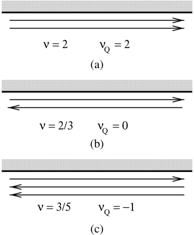
FIG. 1.: Schematic representation of edge states for several different quantum Hall fluids at filling factor $\nu$. The integer $\nu_{Q}$, which specifies the difference between the number of downstream and upstream propagating modes, determines the sign and magnitude of the thermal Hall conductance.

III Hydrodynamic Theory

A central feature of the Luttinger liquid theory of FQHE edges, is the existence of upstream charge carrying modes. Unfortunately, these upstream modes have not been detected experimentally, despite experiments by Ashoori et. al. [7] designed explicitly to observe them. We believe the resolution of this problem lies in the assumption of a clean edge[13, 12]. The clean edge model analyzed in the previous section, contains an artificially high symmetry. In particular, the charge in each of the $n$ different channels is independently conserved. The existence of $n$ conserved charges implies $n$ hydrodynamic modes - those described by (2.4) - some of which propagate upstream.

Impurities which are inevitably present near the edges of any real sample, will destroy this symmetry. One expects that the only remaining conserved charge is the total electrical charge density on the edge. This would imply the presence of only a single long-lived mode, analogous to zero sound in a Fermi liquid. Actually, the situation is somewhat more complicated. As shown in detail in Ref. [11, 13], even with impurity scattering present there are $n-1$ other conserved “charges” at zero temperature, arising from symmetries associated with channel inter-change. In most cases, these other “charges” are neutral with respect to electric charge, and so do not contribute directly to electrical transport. These $n-1$ neutral modes are analogous to quasiparticle excitations in a Fermi liquid. At non-zero temperatures, the “charge” associated with these other $n-1$ modes is no longer conserved, and they decay away by scattering. Thus, at finite temperature, the only remaining conserved charge is indeed total electric charge.

In this paper we focus exclusively on the hydrodynamic regime - at frequency scales below these relevant decay rates. In this regime, we expect only a single propagating hydrodynamic mode, associated with total charge conservation, which propagates downstream. All upstream charge motion is associated with non-conserved charges, and decays away. Observation of upstream charge transport requires a “mesoscopic” experiment in which the sample is smaller than the edge equilibration length.

In the absence of electron-phonon coupling, the electronic energy is also conserved at the edge. Thus, there should be an additional hydrodynamic mode associated with thermal transport. Provided the coupling to the phonons is sufficiently weak, this can be a long lived mode. In this section we develop a simple hydrodynamic theory of charge and heat transport, based on a Boltzmann transport equation. In addition to the hydrodynamic charge mode (zero sound), we identify the single hydrodynamic mode describing the flow of (conserved) energy. This hydrodynamic heat mode leads to a quantized thermal conductance, as in the previous section. Moreover, when $\nu_{Q}<0$, this hydrodynamic mode will be shown to propagate upstream - in the opposite direction to the hydrodynamic charge mode.

Consider first a hydrodynamic description of charge propagation. To formulate a Boltzmann transport theory, we first consider the “collisionless” regime for a clean edge, described by the de-coupled Hamiltonian (2.4). The response of the system to a spatially and temporally varying potential $\Phi$ which couples to the total charge density, $n_{\rho}=\sum_{i}t_{i}n_{i}$, may be obtained from the operator equations of motion as[12]:

$$(\partial_{t}+\eta_{i}v_{i}\partial_{x})n_{i}=\eta_{i}t_{i}\partial_{x}\Phi.$$ (13)

The transport equation (3.1) conserves the charge in each mode. It is the analog of the collisionless Boltzmann equation for a Fermi liquid. Impurity scattering will destroy this conservation and lead to a flow of charge and energy between the channels. This may be incorporated into the transport equation by including a collision term[11, 12]. This Boltzmann description of transport is only valid provided the collisions - or tunneling events - occur incoherently. As discussed above, this implies that the system is in the hydrodynamic regime, at scales longer than equilibration lengths and times. The appropriate linearized transport equation takes the form,

$$(\partial_{t}+\eta_{i}v_{i}\partial_{x})n_{i}+\sum_{j}M_{ij}n_{j}=\eta_{i}t_{i}\partial_{x}\delta\Phi.$$ (14)

The matrix $M_{ij}$ is in general complicated and depends on the detailed nature of the inter-channel scattering. However, $M$ must obey two constraints imposed by conservation laws. (i) In equilibrium there must no net steady state flow of charge between the channels. The equilibrium densities can be extracted by taking a constant potential, $\Phi=\mu$, the chemical potential. Then $n_{i}=v_{i}^{-1}t_{i}\delta\mu$. This implies the condition,

$$\sum_{j}M_{ij}v_{j}^{-1}t_{j}=0.$$ (15)

(ii) The total charge on the edge must be conserved, even out of equilibrium. Since the charge flowing out of channel $i$ is $\sum_{j}t_{i}M_{ij}n_{j}$, this implies

$$\sum_{i}t_{i}M_{ij}=0.$$ (16)

Since the transport equation (3.2) is linear, it may be solved by Fourier transforming, to obtain an eigenvalue problem, with eigenvalues $\omega(q)$. Most of the eigenvalues will correspond to solutions which decay exponentially in time. However, the two constraints, (i) and (ii) above, guarantee that there is one low frequency mode, with $\omega\propto q$ as $q\rightarrow 0$. Specifically, consider a solution to (3.2) of the form

$$n_{i}(x,t)=n_{\rho}{t_{i}v_{i}^{-1}\over\sum_{i}t_{i}^{2}v_{i}^{-1}}e^{i(qx-\omega t)}.$$ (17)

For $q,\omega\rightarrow 0$ this corresponds to “local equilibrium” with a slowly varying charge density $n_{\rho}e^{i(qx-\omega t)}$. Since there is only a single conservation law - total electric charge - we expect this to be the only low frequency solution. Inserting (3.5) into (3.2), multiplying by $t_{i}$ and summing on i, allows the total electric charge $n_{\rho}$ to be related to $\Phi$. The current-charge response function, defined by $J_{\rho}=\Pi_{\rho}(q,\omega)\Phi$, readily follows,

$$\Pi_{\rho}(q,\omega)=G_{H}{v_{\rho}q\over{v_{\rho}q-\omega-i\eta}},$$ (18)

with,

$$v_{\rho}=\nu\left(\sum_{i}t_{i}^{2}v_{i}^{-1}\right)^{-1},$$ (19)

and $G_{H}$ given in (2.3). The response function has a single pole, describing a single hydrodynamic charge mode, which propagates downstream at velocity $v_{\rho}$. This is in contrast to the clean edge, which has $n$ propagating modes, which may also move upstream. As expected, the quantized Hall conductance is given by the $q\rightarrow 0,\omega=0$ limit of the response function.

Consider now a similar analysis for the thermal transport. The transport equation for the energy density in each channel, given a spatially and temporally varying temperature, takes the form,

$$(\partial_{t}+\eta_{i}v_{i}\partial_{x})n_{iQ}+\sum_{j}M^{Q}_{ij}n_{jQ}=\eta_{i}{\pi^{2}\over 3}T\partial_{x}\delta T.$$ (20)

Here we have included a collision term which describes the flow of heat between the channels. Conservation of energy demands that the matrix $M^{Q}$ must satisfy

$$\sum_{i}M^{Q}_{ij}=\sum_{j}M^{Q}_{ij}v_{j}^{-1}=0,$$ (21)

the thermal analogs of conditions (i) and (ii) above. The appropriate generalization of (3.5), which describes a low frequency thermal mode corresponding to local thermal equilibrium, is,

$$n_{Qi}(x,t)=n_{Q}{v_{i}^{-1}\over{\sum_{i}v_{i}^{-1}}}e^{i(qx-\omega t)}.$$ (22)

The thermal response function can then be obtained, as before, employing the thermal Boltzmann equation (3.8). This gives,

$$\Pi_{Q}(q,\omega)=K_{H}{v_{Q}q\over{v_{Q}q-\omega-i\eta}},$$ (23)

where $K_{H}$ is the quantized thermal Hall conductance given in (2.8), and the velocity of the heat mode is

$$v_{Q}=\nu_{Q}\left(\sum_{i}v_{i}^{-1}\right)^{-1}.$$ (24)

Notice that this velocity can be of either sign, depending on $\nu_{Q}$. Thus for $\nu=3/5$, the hydrodynamic heat mode flows upstream in the opposite direction of the charge.

For $\nu=2/3$ the thermal Hall conductance vanishes, and a more detailed analysis of (3.8) is required. This reveals that the thermal transport is diffusive, rather than ballistic, with a response function given by,

$$\Pi_{Q}(q,\omega)=C{\omega qD_{Q}\over{D_{Q}q^{2}-i\omega}},$$ (25)

where $C=(\pi^{2}/3)T\sum_{i}v_{i}^{-1}$ is the edge heat capacity. Although the thermal conductance vanishes, there is a finite thermal conductivity $\kappa=CD_{Q}$. The value of the thermal diffusion constant $D_{Q}$ depends on the details of the scattering matrix $M^{Q}_{ij}$.

IV Experimental Implications

As shown above, the thermal Hall conductance, $K_{H}$, contains important new information about the structure of the edge excitations in the FQHE. In particular, the sign of $K_{H}$ is sensitive to the presence of edge modes which propagate “upstream”. In this section we briefly discuss the feasibility of measuring the Hall thermal conductance. We suggest a particular geometry which should at least enable a measurement of the sign of $K_{H}$.

To extract $K_{H}$ requires measuring the thermal current carried by the edge excitations. Although this is clearly much more challenging than measuring charge transport, a recent experiment by Molenkamp et. al.[14] has demonstrated the feasibility of measuring thermal transport in mesoscopic structures. Specifically, in this experiment the thermal conductance of a quantum point contact (in zero magnetic field) was extracted. The trick was using additional point contacts as “thermometers”, to measure the local temperature of the electron gas on either side of the point contact. The additional point contacts were biased on the edge of a step between two plateaus, so that they would have a large, temperature independent thermopower of order $40\mu V/K$[15]. Then, by measuring the voltage across these additional point contact thermometers the local temperature change was extracted. In Molenkamp’s experiment, the thermal current was estimated from the change in temperature by estimating the heat capacity of the electron gas. This allowed for a determination of the thermal conductance and Peltier coefficient of the point contact which agreed favorably with theoretical expectations.

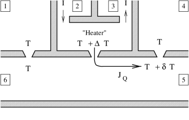
FIG. 2.: Proposed geometry for measurement of the thermal Hall conductance. The heat generated by passing a current between contacts 2 and 3, is detected by two additional point contacts, upstream (1-6) and downstream (4-5) along the edge.

It should be possible to adapt this technique to measure the thermal transport of quantum Hall edge states. As a concrete example, consider the geometry sketched in Fig. 2. As in the experiment by Molenkamp et. al., the sample can be heated locally by driving a small electric current through the electron gas. Specifically, a current between contacts 2 and 3 (see Figure) would locally heat the edge of the quantum Hall fluid. Alternatively, it might be possible to heat the edge directly by coupling in a local RF probe[16]. This local heating will be carried away by the edge states, either raising the temperature of the downstream or upstream edge, depending on the sign of $K_{H}$. This temperature change can then be detected by measuring the voltages across the point contact thermometers.

While this measurement might not be suitable to extract the magnitude of $K_{H}$, it should be adequate to determine the direction of heat propagation - and hence the sign of $K_{H}$. For this, one need only detect an asymmetry in the temperature change of the upstream and downstream edges. For integer quantum Hall states, and fractional states at filling factors such as $\nu=1/3,2/5$, the heat should flow downstream, resulting in a temperature increase at the downstream thermometer only. On the other hand, for filling $\nu=3/5$, since $K_{H}$ is negative, heat flows “upstream”, so the temperature increase should be detectable at the upstream thermometer. For $\nu=2/3$, the heat is predicted to diffuse along the edge. The temperature increases should then be the same at the up and downstream thermometers, but smaller in magnitude.

On sufficiently long length scales, the edge states will thermally equilibrate with the phonons in the substrate. It is thus crucial that the heater and thermometer are closer together than the electron-phonon thermal equilibration length. While this equilibration length has not been measured, we expect it to be quite long. Energy relaxation rates have been measured for 2 dimensional electron gases in GaAs[17, 18] in zero magnetic field. At $1^{\circ}K$ relaxation times of order $20ns$ are found, which suggests an equilibration length of upwards of $100\mu m$. At low temperatures, the interaction between electrons and the lattice in GaAs is dominated by the piezoelectric coupling to acoustic phonons and the relaxation rate decreases as the temperature is lowered[18, 19]. Thus, we suspect that lattice thermalization will not be a problem in the proposed edge state experiment.

V Conclusion

We have shown that the thermal conductance of a quantum Hall edge state is universal and quantized: $K_{H}=\nu_{Q}K_{0}$ with $K_{0}=(\pi^{2}/3)(k_{B}^{2}/h)T$. The integer $\nu_{Q}$ specifies the difference between the number of downstream and upstream edge modes. Moreover, the quantization of $K_{H}$ was shown to be robust, valid in the presence of interactions and impurity scattering at the edge. We also expect the quantization to hold for an edge with a slowly varying confinement potential, which may have channels in addition to those required by the Luttinger liquid theory[20]. Since the additional edge channels come in pairs - one upstream and one downstream - they do not change $\nu_{Q}$. On sufficiently long length scales, so that all edge modes are equilibrated, we predict only a single hydrodynamic charge mode and a single heat mode. These two hydrodynamic modes carry the charge and thermal currents, leading to the quantized conductances.

In the FQHE, the thermal Hall conductance $K_{H}$ contains additional information about the microscopic edge structure, not present in the electrical conductance. For $\nu=3/5$, we predict that $K_{H}$ is negative, due to the presence of “upstream” propagating edge modes. A measurement of the sign of $K_{H}$ would thus provide a critical and nontrivial test of current edge state theories.

- [1] B.I. Halperin, Phys. Rev. B 25, 2185 (1982).
- [2] E.M. Lifshitz and L.P. Pitaevskii, Physical Kinetics (Pergamon Press, New York 1981), p. 244.
- [3] U. Sivan and Y. Imry, Phys. Rev. B 33, 551 (1986).
- [4] X.G. Wen, Phys. Rev. B 43, 11025 (1991); Phys. Rev. Lett. 64, 2206 (1990). X.G. Wen, Phys. Rev. B 44 5708 (1991).
- [5] C.L. Kane and M.P.A. Fisher, “Thermal Transport in a Luttinger Liquid,” Phys. Rev. Lett., in press.
- [6] A. H. MacDonald, Phys. Rev. Lett. 64, 222 (1990); M. D. Johnson and A. H. MacDonald, Phys. Rev. Lett. 67, 2060 (1991).
- [7] R.C. Ashoori, H. Stormer, L. Pfeiffer, K. Baldwin and K. West, Phys. Rev. B 45, 3894 (1992).
- [8] F.D.M. Haldane, Phys. Rev. Lett. 51, 605 (1983); B.I. Halperin, Phys. Rev. Lett. 52, 1583 (1984).
- [9] See X.G. Wen and A. Zee, Phys. Rev. B 46, 2290 (1992), and references therein.
- [10] N. Read, Phys. Rev. Lett. 65, 1502 (1990).
- [11] C.L. Kane and M.P.A. Fisher, Phys. Rev. B 51, 13449 (1995).
- [12] C.L. Kane and M.P.A. Fisher, Phys. Rev. B 52, 17393 (1995).
- [13] C. L. Kane, M.P.A. Fisher and J. Polchinski, Phys. Rev. Lett. 72, 4129 (1994).
- [14] L.W. Molenkamp et. al., Phys. Rev. Lett. 68, 3765 (1992).
- [15] P. Streda, J. Phys. Condens. Matter 1, 1025 (1989).
- [16] L. Kouwenhoven, private communication.
- [17] A.S. Dzurak, et. al., Phys. Rev. B 45, 6309 (1992).
- [18] Y. Ma, et. al., Phys. Rev. B 43, 9033 (1991).
- [19] B. K. Ridley, Rep. Prog. Phys. 54, 169 (1991).
- [20] D.B. Chklovskii, Phys. Rev. B 51, 9895 (1995).