Localization Bounds for an Electron Gas

Abstract Mathematical analysis of the Anderson localization has been facilitated by the use of suitable fractional moments of the Green function. Related methods permit now a readily accessible derivation of a number of physical manifestations of localization, in regimes of strong disorder, extreme energies, or weak disorder away from the unperturbed spectrum. The present work establishes on this basis exponential decay for the modulus of the two–point function, at all temperatures as well as in the ground state, for a Fermi gas within the one–particle approximation. Different implications, in particular for the Integral Quantum Hall Effect, are reviewed.

1. Introduction

1.a The localization condition

This is a report on recent progress in the mathematical analysis of Anderson localization. The simplifications which have been made in its derivation permit now to access a number of interesting properties of systems with disorder, by methods which are both mathematically rigorous and not excessively complicated. The report includes some new technical statements, but we recall also a number of previously known results, derived by various other authors, in order to present a more complete picture of the physically motivated questions which can be addressed by related mathematical methods.

Anderson localization was first discussed in the context of the conduction properties of metals ([1, 2]), but the mechanism is of relevance in a variety of other situations (e.g., [3]). The basic phenomenon is that disorder can cause localization of electron states (or normal modes — in other systems) and thereby affect properties like: time evolution (non–spreading of wave packets), conductivity (in response to electric field), Hall currents (in the presence of both magnetic and electric field), and statistics of the spacing between nearby energy levels.

In the electron gas approximation the system of electrons in a crystal is modeled by a gas of Fermions moving on a lattice. We focus here on systems with homogeneous disorder, which otherwise are periodic or translation invariant, at least up to gauge transformations. The excitations of the system are described by an effective one–body Hamiltonian, which consists of a short–range hopping term and a local potential. The one–particle Hamiltonian is a self–adjoint operator with matrix elements of the form

$$H=K_{x,y}+U^{per}_{x}+\lambda V_{x}\;,$$ (1.1)

acting in the Hilbert space $\ell^{2}(\mbox{\boldmath$Z$}^{d})$, where $K_{x,y}$ is a short–range hopping term, $U^{per}_{x}$ a periodic potential, and $\lambda V$ a random potential expressing the disorder (impurities) with a tunable strength parameter $\lambda$.

We shall not discuss here the validity of the one–particle approximation, or that of the linear response theory. Instead, we focused on the analysis within such frameworks. In particular, we shall demonstrate how resolvent estimates can be used to address a number of physically motivated questions.

For $K_{x,y}$ we consider the following two cases:

No magnetic field: $K_{x,y}$ depend only on the difference $(x-y)$.

Constant magnetic field: There is some ambiguity in the definition of the magnetic flux, since flux differences of $h/e$ can be induced, or compensated for, by gauge transformations. For concreteness sake, let us restrict to the operators of the form:

$$K_{x,y}\ =\ {\rm e}^{-{\rm i}{\cal A}_{x,y}}\ \delta_{|x-y|,1}$$ (1.2)

with a phase ${\cal A}_{x,y}$ which is an antisymmetric function of the oriented bonds, $b=\{x,y\}$. (${\cal A}_{x,y}$ can be viewed as the line integral of the “vector potential” $\times(-e/\hbar)$ along the direct path from $x$ to $y$). The magnetic flux through a plaquette $P$ is taken to be

$$B_{P}\ =\ -\frac{\hbar}{e}\sum_{b\in\partial P}{\rm Arg\,}(K_{b})\;,$$ (1.3)

with the argument function interpreted through its principal branch, i.e., $-\pi<{\rm Arg\,}z\leq\pi$. At non-zero field, translation invariance is possible only in the sense of magnetic translations, which combine shifts with gauge transformations, i.e. are unitaries of the form

$$U(a)|x\rangle\ =\ {\rm e}^{-{\rm i}\varphi_{a}(x)}|x+a\rangle\;.$$ (1.4)

In such cases, $K=U(a)KU(a)^{*}$ implies ordinary translation invariance for gauge invariant quantities, such as $|K_{x,y}|$ and $|\langle x|(K-E-{\rm i}\eta)^{-1}|y\rangle|$. (The fact that the composition law for the magnetic shifts provides only a projective representation of the translation group does not affect our analysis.)

The potential $V$ is realized as a collection of independent identically distributed random variables $V_{x}$, whose probability distribution may be of the form $r(v)dv$ with $r(v)$ a bounded probability–density function. (These conditions may be relaxed: the results described below are valid also for a broad class of correlated randomness, more singular probability distributions for $V$, and Hamiltonians with off diagonal disorder, i.e., randomness in $K_{x,y}$.)

Of central importance in the analysis is the Green function, i.e., the kernel of the resolvent operator:

$$G(x,y;E+{\rm i}\eta)=\langle x|{1\over H-E-{\rm i}\eta}|y\rangle\ \ .$$ (1.5)

The behavior of this function at $\eta=0+$ reveals a great deal about the spectral properties of the Hamiltonian (e.g., discrete versus continuous spectrum), the nature of its eigenfunctions (localized or extended), and the response of the system (e.g., to electric fields) at the linear–response level.

A technically convenient signature of localization is a bound on the fractional moments of $G(0,x;E)$. The explicit condition is that for energies $E$ in an interval $[a,b]$ and some $0<s<1$,

$$\mbox{\boldmath$E$}(|G(x,y;E+{\rm i}\eta)|^{s})\leq C^{s}{\rm e}^{-s\mu|x-y|}\;,$$ (1.6)

for all $\eta\neq 0$. Here and henceforth $E$ represents the average over the randomness and $C<\infty$ and $\mu>0$ are constants which may change from line to line, but are to be understood as independent of $\eta$. The value of $s$ is of little consequence (if the condition (1.6) holds for some $s$ then by Hölder inequality it extends to all smaller $s>0$), but the restriction $s<1$ permits to avoid the divergence explained below.

The condition (1.6) was established for a broad class of systems, in any dimension, under any of the three conditions: 1) high disorder, 2) extreme energies [4], and 3) weak disorder [5] away from the spectrum of the unperturbed operator ($\lambda=0$), see Figure 1. Localization is known also to occur at the band edges (case 4), for which it can be proven [6, 7] by the multiscale approach of Fröhlich and Spencer [8]. However, in this more delicate situation condition eq. (1.6), which leads to the implications discussed below, has not been established yet. Neither has the condition been derived in the continuum (for which localization results can be found in refs. [9, 10, 11, 12, 3, 13, 14, 15]).

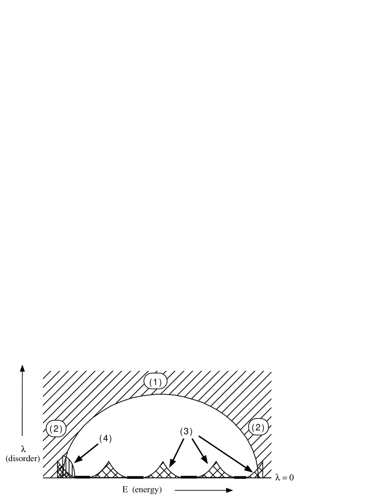
Figure 1: Different regions (schematically) in which localization occurs for an operator of the form $H=H_{o}+\lambda V_{random}$: 1) high disorder, 2) extreme energies, 3) weak disorder, away from the spectrum of $H_{o}$, and 4) band edges. The fractional moment methods have been developed for the first three regimes.

We shall recapitulate below why eq. (1.6) can be viewed as a natural technical expression of localization, and present a heuristic derivation along the lines of [4]. First, however let us list some of its implications.

1.b Physical implications of the resolvent condition

There is a growing list of readily identifiable physical properties of an electron gas which follow from eq. (1.6), some of which have not been derived without it.

A new statement which is added here to that list is the exponential decay of the two–point function in the ground state $|0\rangle\rangle$ if the Fermi energy, $E_{F}$, falls within a range of energies for which eq. (1.6) holds. In terms of Fock–space Fermionic operators

$$\mbox{\boldmath$E$}(|\langle\langle 0|\psi^{\dagger}(x)\psi(y)|0\rangle\rangle|)\leq C{\rm e}^{-\mu|x-y|}\;,$$ (1.7)

or, in terms of the relevant one–particle spectral projection $P_{\leq E_{F}}$, on the energy range $(-\infty,E_{F}]$,

$$\mbox{\boldmath$E$}(|\langle x|P_{\leq E_{F}}|y\rangle|)\leq C{\rm e}^{-\mu|x-y|}\;.$$ (1.8)

Remark: i) If $E_{F}$ falls in a band of extended states the above kernel decays by only a power law.

ii) The derivation of the exponential decay, given below, does not require eq. (1.6) to hold for all the energies below $E_{F}$. Thus, it applies also to the case in which the Fermi level is in a localized regime above a number of bands of extended states.

iii) The decay presented in eq. (1.8) has interesting implications on electrical conductance, both in the absence and in the presence of magnetic field (Hall conductance), which are discussed below.

Before we turn to the derivation of the conditions (1.6) and (1.8), let us list some other physically meaningful implications of eq. (1.6), some derived by other authors, which it may be useful to have listed together. These include:

• Pure–point spectrum: the spectrum of the operator $H$ in the interval $[a,b]$ almost surely consists only of (non–degenerate) eigenvalues with exponentially localized eigenfunctions.

The implication is through either the dynamical localization expressed in eq. (1.9) or the Kotani argument [16], as further explained by Simon-Wolff [17]. This argument yields the useful principle that those decay properties of the resolvent which hold for almost all energies in some interval — in a sense which is not affected by randomizations which refresh the site potentials — are typically manifested also by all the eigenfunctions the operator may have in that interval. (The property of interest here is the exponential decay.)

• Dynamical localization: assuming eq. (1.6), wave packets of states with energy in the range $[a,b]$ do not spread. The key estimate is ([5])

  $$\mbox{\boldmath$E$}(\sup_{t}|\langle x|P_{[a,b]}{\rm e}^{-{\rm i}tH}|y\rangle|)\leq C{\rm e}^{-\mu|x-y|}\ \ .$$ (1.9)

One may note that eq. (1.9) is a stronger statement than the exponential localization of eigenfunctions (it was not available before eq. (1.6)). Implicit in its derivation is an extension which permits to replace $e^{-itH}$ by an arbitrary bounded function $f(H)$. Expressed in terms of the eigenfunctions, with energies $E_{n}$ the assertion is:

$$\mbox{\boldmath$E$}(\sum_{E_{n}\in[a,b]}|\psi_{n}(x)||\psi_{n}(y)|)\leq C{\rm e}^{-\mu|x-y|}\;.$$ (1.10)

• Absence of level repulsion: Minami [18] proved that the localization condition eq. (1.6) implies that the local distribution of the energy levels in the interval $[a,b]$, for the system in $[-L,L]^{d}$, converges (as $L\to\infty$) to the Poisson law — i.e., the energy levels appear to be independently distributed.

The decay presented in eq. (1.7) has interesting implications on conductivity, both in the absence and in the presence of magnetic field.

We refer here to the conductivities as given by linear–response calculations. We shall not address here the interesting questions concerning the validity of such approximations, and the role of edge currents.

• Vanishing of the d.c. electrical conductivity in the absence of magnetic field: We shall see below that, for any dimension,

  $$\mbox{condition (\ref{eq:gs})}\ \Longrightarrow\ \sigma_{i,j}(E_{F})\ =\ 0\ \ \mbox{ (for $E_{F}\in(a,b)$)},$$ (1.11)

  where $\sigma$ is the d.c. electrical conductivity of an electron gas with Fermi energy $E_{F}$, at the zero temperature limit and at zero magnetic field, based a linear response calculation (Kubo formula):

  $$\sigma_{i,j}(E_{F})=\lim_{\eta\downarrow 0}{\eta^{2}\over\pi}\sum_{x\in\mbox{\boldmath$Z$}^{d}}x_{i}x_{j}\mbox{\boldmath$E$}(|G(0,x;E_{F}+{\rm i}\eta)|^{2})\;.$$ (1.12)

Let us remark that this expression for the conductivity follows from the more standard Kubo formula ([2, 19]) under the assumption of finite conductivity. (For completeness, we present the argument in Appendix  ??.Localization Bounds for an Electron Gas.) An earlier proof of the vanishing of $\sigma$ (in this form) was provided in ref. [8] for the regime covered by the “multiscale analysis”.

In the presence of magnetic field, one is interested in the Hall conductance. The linear response calculation (see Appendix  ??.Localization Bounds for an Electron Gas) is facilitated by the condition

$$\mbox{\boldmath$E$}\Bigl{(}\sum_{x\in\mbox{\boldmath$Z$}^{d}}|x|^{2}|\langle 0|P_{\leq E}|x\rangle|^{2}\Bigr{)}<\infty\;,$$ (1.13)

which is implied by eq. (1.8). The Kubo formula for this situation is

$$\sigma_{i,j}(E)={\rm i}\,{\rm Tr}(P_{\leq E}[[x_{i},P_{\leq E}],[x_{j},P_{\leq E}]])\;.$$ (1.14)

• Integral Quantum Hall Effect (2D): Bellissard, van Elst, and Schulz-Baldes [20] (BES) proved that if eq. (1.13) holds for a two–dimensional system then at the corresponding Fermi energy the Hall conductance $\sigma_{1,2}(E_{F})$ is an integer $\times e^{2}/h$ and it is constant throughout intervals, like $[a,b]$ of eq. (1.9), in which the localization length is is uniformly bounded.

Results leading to this conclusion were also developed by Avron, Seiler and Simon  [21] (AS²).

To put this result in a clearer perspective, consider the continuum case of a Landau Hamiltonian weakly perturbed by a random potential:

$$H\ =\ \frac{1}{2}\left(\frac{{\rm i}}{\hbar}\underline{\nabla}+e\frac{\underline{B}\wedge\underline{x}}{2}\right)^{2}+\lambda U_{random}(x)$$ (1.15)

where $U_{random}(x)$ could be of the form $U_{random}(x)=\sum_{j}\eta_{j}V(x-x_{j})$, with $\{x_{j}\}$ randomly distributed points and $\{\eta_{j}\}$ independent random coefficients. Had all the results which are proven for the lattice Hamiltonians been true in this case, one could deduce that for small $\lambda$ the Hall conductance, as a function of the Fermi energy exhibits several plateaux, increasing as $\sigma_{Hall}=(e^{2}/h)n$. It would indeed be of interest to see an extension to the continuum of the localization analysis discussed here.

The argument of BES [20] is based on a number of sophisticated results of non–commutative geometry (in particular, theory developed by A. Connes). To make these results more transparent, we include below a direct and simple derivation of the implication of eq. (1.8) for the IQHE. The discussion incorporates ideas which were developed by AS² [21], discussed here in the context of operators with random potentials under the localization condition eq. (1.8).

2. Localization Bounds for the Resolvent

To convey the key arguments leading to localization bounds let us review the derivation of equation eq. (1.6) for the situation with high disorder, or at extreme energy (cases 1) and 2) in Fig. 1). Furthermore, let us consider the case where the magnetic field $B$ is either zero or constant, $K_{x,y}$ is restricted to the nearest–neighbor pairs (e.g., $K_{x,y}=$ the incidence matrix), and $U^{per}_{x}\equiv 0$. The equations defining the resolvent (with $y=0$ and ${\rm i}\eta$ absorbed in $E$) is: $(H-E)G(x,0;E)=\delta_{x,0}$, or:

$$(E-\lambda V_{x})G(x,0;E)\ =\ \sum_{n\in\mbox{\boldmath$Z$}^{d},|n|=1}K_{x,x+n}\;G(x+n,0;E)\;-\;\delta_{x,0}\;.$$ (2.1)

The solution of this equation does not propagate well (it attenuates, or decays exponentially) in regions where $E-\lambda V_{x}$ falls out of the spectral range of the hopping operator seen on the right side, i.e., where $|E-\lambda V_{x}|>2d$. If $\lambda$ is large enough (or $E$ is very large), most of the lattice will belong to this attenuation set, and one may expect $G(x,0;E)$ to decay exponentially in $|x|$, indicating exponential localization.

The big gap in this intuitive argument is that one still needs to address the possible tunneling between the sparse sites at which $|E-\lambda V_{x}|\leq 2d$. This gap was closed by the “multiscale analysis” of ref. [8], which was developed to handle the technical problems caused by possible resonances, manifested through small denominators. An alternative approach is to look at suitable moments of $G(x,0;E)$, with the hope that the averaged quantities will be informative enough. Here the small denominator problem shows up as follows: for $H$ taken to be a finite matrix (and $E$ real),

$${\rm Av}(|G(x,0;E)|)=\infty$$ (2.2)

where the average is either over the energy $E$, integrated over any interval which intersects the spectrum, or over the values of $V_{x}$. The latter singularity is explained by “rank–one perturbation formulae” (or, alternatively, Cramer’s rule), e.g.,

$$G(x,x;E)=\frac{1}{\widehat{G}(x,x;E)^{-1}+\lambda V_{x}}$$ (2.3)

where $\widehat{G}(x,x;E)$ — the value of $G(x,x;E)$ for $V_{x}$ changed to $0$ — does not depend on $V_{x}$. In a system in which $V_{x}$ is independent from the values of the potential at other sites, there will be rare resonant situations, in which the denominator in eq. (2.3) is very small. Despite its rarity, this phenomenon leads to “$1/t$ tail” in the distribution of $|G(x,x;E)|$, as well as of the other matrix elements, and to the divergence of the mean values expressed by eq. (2.2).

Once the nature of the singularity is understood, one may see how to keep it from obscuring the picture. The key observation is that this singularity does not cause blowups in fractional moments, i.e., averages of $|G(x,0;E)|^{s}$ with any $0<s<1$. Averaging both sides of equation (2.1) raised to such a power $0<s<1$, one may obtain the following relation (with the help of a decoupling argument, discussed in [4, 5])

$$c\ \mbox{\boldmath$E$}(|\lambda V_{x}-E|^{s})\ \mbox{\boldmath$E$}(|G(x,0;E)|^{s})\leq\sum_{n\in\mbox{\boldmath$Z$}^{d},|n|=1}\mbox{\boldmath$E$}(|G(x+n,0;E)|^{s})\ +\ \delta_{x,0}\;,$$ (2.4)

with $c$ a finite constant depending on the distribution of the random potential. In the above relation the effect of the rare resonances is averaged out, and the simple argument indicated below eq. (2.1) can be followed in a conclusive way. When

$$\gamma=\frac{2d}{c\;\mbox{\boldmath$E$}(|\lambda V_{x}-E|^{s})}<1$$ (2.5)

eq. (2.4) implies that $\mbox{\boldmath$E$}(|G(x+n,0;E)|^{s})$ is a strictly subharmonic function on the lattice (its value at $x$ is less that $\gamma(<1)$ times its average over neighbors). This readily implies the exponential decay expressed in (1.6), for strong disorder ($\lambda$ large), and at extreme energies. This argument leads to the following result.

Theorem 1

For a random Hamiltonian as in eq. (1.1), with $V_{x}$ independent variables having the probability distribution $r(v)dv$ with $r(v)$ bounded, if for some $0<s<1$ and $\mu>0$

$$\lambda>2\|r\|_{\infty}\Big{(}{2\over 1-s}\sum_{x\in\mbox{\boldmath$Z$}^{d}}|K_{0,x}|^{s}{\rm e}^{\mu|x|}\Big{)}^{1/s}\;,$$ (2.6)

then

$$\mbox{\boldmath$E$}(|G(x,y;z)|^{s})\leq C{\rm e}^{-\mu|x-y|}\;,$$ (2.7)

uniformly in $z\in\mbox{\boldmath$C$}\setminus\mbox{\boldmath$R$}$.

The complete derivation is given below in Appendix  ??, where we reproduce in a slightly streamlined fashion the argument of ref. [4], and derive the exponential decay in a more general setup, in which the probability distribution is not required to have a density with respect to $dv$. This approach can also be applied to other regimes, where the resolvent can be studied through other equations, e.g., the relation to the unperturbed resolvent operator: $G=G_{o}-G_{o}\lambda VG$ ([5]), yielding bounds which are uniform in the two natural cutoffs: finite volume, and imaginary energy shift i$\eta$ ([22]).

3. Exponential Decay for the Two–Point Function

We now turn to the implication of eq. (1.6) for the two–point function, which for temperature $T\geq 0$ is given by

$$\langle\psi^{\dagger}(x)\psi(y)\rangle_{T}=\mbox{\boldmath$E$}(\langle x|\theta_{T}(H-E_{F})|y\rangle)\;,$$ (3.1)

with the Fermi distribution $\theta_{T}(u)=(1+\exp(u/T))^{-1}$. For $T=0$: $\theta_{0}(u)=I[u\leq 0]$.

At $T>0$ this function always exhibits exponential decay, but at a rate for which the general bound — independent of $V$ and $E_{F}$ — vanishes with $T$:

$$|\langle x|\theta_{T}(H-E_{F})|y\rangle|\leq C{\rm e}^{-\gamma T|x-y|}\;,$$ (3.2)

(as follows from Theorem 3 below). We can say more under the localization criterion eq. (1.6):

Theorem 2

If eq. (1.6) holds at the Fermi energy $E_{F}$ then the two–point function decays exponentially fast at the ground state (filled ‘Fermi sea’), and also at positive temperatures — with the correlation length ($\xi$) staying uniformly bounded as $T\to 0$, i.e.

$$\mbox{\boldmath$E$}(|\langle x|\theta_{T}(H-E_{F})|y\rangle|)\leq C{\rm e}^{-|x-y|/\xi}$$ (3.3)

for all $T>0$, and also

$$\mbox{\boldmath$E$}(|\langle x|P_{\leq E_{F}}|y\rangle|)\leq C{\rm e}^{-|x-y|/\xi}\;$$ (3.4)

(corresponding to the case $T=0$).

Proof: To extract the information from the resolvents, it is convenient to employ the contour integral representation. For the projection $P_{\leq E_{F}}$ we chose the path to consist of segments joining $-\infty-{\rm i},\,E_{F}-{\rm i},\,E_{F}+{\rm i},\,-\infty+{\rm i}$. Splitting the integral, we get

$$P_{\leq E_{F}}=Q_{1}(H-E_{F})+Q_{2}(H-E_{F})\;,$$ (3.5)

with

$$Q_{1}(z) = {1\over 2\pi}\int_{-1}^{1}d\eta\,{1\over{\rm i}\eta-z}\;,$$ (3.6)

$$Q_{2}(z) = {1\over 2\pi{\rm i}}\int_{-\infty}^{0}du\Bigl{[}{1\over u-{\rm i}-z}-{1\over u+{\rm i}-z}\Bigr{]}\;.$$ (3.7)

(due to the randomness, the probability of there being an eigenvalue exactly at the energy $E_{F}$ is zero ([17]), a fact immediate from (1.6)).

For $T>0$, $\theta_{T}(z)$ has poles at ${\rm i}\pi T\times${odd integers}, which grow dense on the imaginary axis as $T\to 0$, with residues equal $(-T)$. Evaluating the Cauchy integral along the boundary $\Gamma$ of the strip $|{\rm Im}\,z|\leq\eta$ with $\eta=[\frac{1}{2\pi T}]\;2\pi T\approx 1$), where $[X]$ denotes the integral part of $X$, one finds $\theta_{T}(H-E_{F})=\theta_{T,1}(H-E_{F})+\theta_{T,2}(H-E_{F})$ with

$$\theta_{T,1}(z) = {T}\sum_{n{\em odd};|n\pi T|<\eta}{1\over{\rm i}n\pi T-z}\;,$$ (3.8)

$$\theta_{T,2}(z) = {1\over 2\pi{\rm i}}\int_{\Gamma}dw\,\theta_{T}(w){1\over w-z}$$ (3.9)

$$= {1\over 2\pi{\rm i}}\int_{-\infty}^{\infty}du\,\theta_{T}(u)\Bigl{[}{1\over u-{\rm i}\eta-z}-{1\over u+{\rm i}\eta-z}\Bigr{]}\;.$$

The sum defining $\theta_{T,1}(H-E_{F})$ looks, at small $T$, like a discrete approximation of the integral seen in $Q_{1}(H-E_{F})$.

In each case ($T=0$ and $T>0$), one may expect the first term to be the more delicate one, since it involves resolvents at arbitrarily small distances (of the complex energies) from the real axis. Indeed, it is at that point that the assumed condition eq. (1.6) enters. For the more regular terms, $Q_{2}(H-E_{F})$ and $\theta_{T,2}(H-E_{F})$, a starting point is provided by the Combes–Thomas estimate (reproduced below in eq. (D.3)), however we need to improve on that in order to address the question of the convergence of the resulting integrals. (This question can be avoided in case the potential is uniformly bounded ($H\geq E_{0}>-\infty$) by closing the contour at any point below $E_{0}$.)

More explicitly, we estimate the first term as follows:

$$\mbox{\boldmath$E$}(|\langle x|Q_{1}(H-E_{F})|y\rangle|) \leq {1\over 2\pi}\int_{-1}^{1}d\eta\mbox{\boldmath$E$}(|G(x,y;E_{F}+{\rm i}\eta)|)$$ (3.10)

$$\hskip-56.9055pt\leq{1\over 2\pi}\int_{-1}^{1}d\eta\,\eta^{-(1-s)}\mbox{\boldmath$E$}(|G(x,y;E_{F}+{\rm i}\eta)|^{s})\leq C{\rm e}^{-\mu|x-y|}\;,$$

where we combined the assumed resolvent condition eq. (1.6), with the general operator bound $|G(x,y;E_{F}+{\rm i}\eta)|\leq\eta^{-1}$. A similar estimate holds for $\mbox{\boldmath$E$}(|\langle x|\theta_{T,1}(H)|y\rangle|)$, the difference being that the integral over $\eta$ is replaced by a corresponding Riemann sum.

The exponential decay for the corresponding second pair of terms, $\mbox{\boldmath$E$}(|\langle x|Q_{2}(H-E_{F})|y\rangle|)$ and $\mbox{\boldmath$E$}(|\langle x|\theta_{T,2}(H-E_{F})|y\rangle|)$, is a direct consequence of the following general result, whose proof is given here in Appendix  ??.

Theorem 3

Let $H$ be as in eq. (1.1) and $F$ be a function analytic and bounded in the strip $|{\rm Im}\,z|<\eta$ (by $\|F\|_{\infty}$). Then

$$|\langle x|F(H)|y\rangle|\leq 18\sqrt{2}\|F\|_{\infty}\ {\rm e}^{-\mu|x-y|}$$ (3.11)

for any $\mu$ such that the quantity $b(\mu)=\sum_{x\in\mbox{\boldmath$Z$}^{d}}|K_{0,x}|$ $({\rm e}^{\mu|x|}-1)$ satisfies $b(\mu)\leq\eta/2$.

In fact, this result relies on $F$ having a representation (D.2) analogous to (3.7, 3.9).

$\Box$

4. Hall – Kubo conductance as a charge–transport index

The analysis described above applies in particular to systems with a uniform magnetic field. This case has, of course, attracted a great deal of attention due to the remarkable phenomenology associated with the Quantum Hall Effect (QHE). The Integral QHE ([23]) (unlike the Fractional case [24]) is understood now to be accountable for within the electron-gas picture, in which the particles (or excitations) are subject to a one-particle effective Hamiltonian of the type considered here (see, e.g. [25]).

It has been pointed out that under suitable circumstances the values of $\sigma_{H}h/e^{2}$ express topological indices, which would account for both the observed integer values and for the robustness of the phenomenon of IQHE ([26, 27, 28, 29]). Curiously, the robustness is re–expressed in the fact that similar conclusions are reached through different explanations, in which the topological aspect of Hall conductance appears in different disguises.

In this section we recount one of the approaches to Hall conductance in two dimensions, employing the charge transport index which was introduced and used very effectively by Avron, Seiler and Simon (AS²) [21]. The only addition in this paper to the above work is the derivation of the exponential decay of the kernel of the projection operator $P_{\leq E_{F}}$, eq. (3.4), which (in a weaker form, e.g. fast enough power law) is essential for the integrality of Hall conductance. Another approach, which was developed by Bellissard, van Elst, and Schulz-Baldes (BES) [20] will be mentioned in the next section. BES proceeded along a slightly different path, employing the Chern–character view of the Hall conductance and theorems proven in the context of “non-commutative geometry”. The latter work had a more intense focus on random systems, and stated conditions under which Hall plateaux exist. However, as noted in both works, the seemingly parallel tracks actually meet, through a formula discovered by A. Connes.

The first step may be the formulation of a mathematical expression for the Hall conductance within the model considered here. One intriguing option is based on the charge pump mechanism proposed by Laughlin [30]. Consider a system in which the charges are confined to a plane (e.g., a suitable interface), and the magnetic field is changed through an adiabatic process which results in the increase of the flux through a finite region $D$ by $\Delta\Phi$. Changes in the magnetic field are accompanied by an electric field ($\underline{E}$), including in the area surrounding $D$, and current — whose density we denote by $\underline{J}$. The rate of charge transport across a contour ${\mathcal{C}}$ encircling $D$ is

$$\frac{\Delta Q}{\Delta t}\ = \ \oint_{\mathcal{C}}\underline{J}\cdot\underline{n}\ d\ \ell$$ (4.1)

$$= \ \sigma_{D}\oint_{\mathcal{C}}\underline{E}\cdot\underline{n}\ d\ \ell\ -\sigma_{H}\oint_{\mathcal{C}}\underline{E}\cdot\underline{d\ \ell}\;,$$

where $\sigma_{D}$ and $\sigma_{H}$ are elements of the bulk (homogenized) conductivity tensor (within the plane)

$$\underline{J}=\sigma\underline{E}\;,\;\;\sigma\ =\ \left(\begin{array}[]{cc}\sigma_{D}&-\sigma_{H}\\ \sigma_{H}&\sigma_{D}\end{array}\right)\;.$$ (4.2)

The last integral on the right side of eq. (4.1) (the induced electromotive force) is tied, by Lenz’s law, to the flux change $-d\Phi/dt$. The first term vanishes in situations in which the direct conductivity ($\sigma_{D}$) is zero. In that case, the integral over time yields an expression for the Hall conductance as the ratio of the transported charge to the flux change:

$$\sigma_{H}=\frac{\Delta Q}{\Delta\Phi}\;.$$ (4.3)

One may note that it might be easier to analyze increments of flux in multiples of $h/e$, since the addition of such a flux quantum can be accomplished by means of a gauge transformation, e.g.,

$$U_{a}\ \psi(x)\ =\ e^{-{\rm i}\theta_{a}(x)}\psi(x)$$ (4.4)

where $a\ (\notin\mbox{\boldmath$Z$}^{2})$ is the location of the added flux line and $\theta_{a}(x)$ is the angle of sight from $a$ to $x$ (${\rm Arg\,}(x-a)$, in the terminology of the complex plane). The natural geometry for a charge pump based on this mechanism is the Corbino disk, where the transfer occurs between two conducting rings, with the region between them filled by material whose microscopic structure is modeled by the system discussed in this paper. Detailed analysis of this effect was presented in the works of Laughlin [30] and Halperin [31].

Motivated by considerations related to the above discussion, Avron, Seiler and Simon [21] proposed an interesting representation of the Hall conductance in the model discussed here, in the $T=0$ limit. They prove that if the two–point function $\langle x|P_{\leq E_{F}}|y\rangle$ decays fast enough, then in a well defined sense only a finite number of states are moved across the Fermi level. The mathematical expression of this is an index, which for a pair of projections $P$ and $Q$ of compact difference is defined as:

$${\rm Index\,}(P,Q)\ :=\ \dim\left\{\psi\in{\mathcal{H}}\ {\Huge|}\ \begin{array}[]{c}P\psi=\psi\\ Q\psi=0\end{array}\right\}\ -\ \dim\left\{\psi\in{\mathcal{H}}\ {\Huge|}\ \begin{array}[]{c}P\psi=0\\ Q\psi=\psi\par\end{array}\right\}\;,$$ (4.9)

(if $(P-Q)$ is a compact operator, the above dimensions are finite).

Assuming that the above charge transport index coincides also with the charge transferred in the course of an adiabatic transition from $H$ to $UHU^{*}$, ($\Delta\Phi=h/e$), AS² take for the Hall conductance the quantity

$$\sigma_{H}\ =\ \frac{e}{h/e}\ \mbox{\boldmath$E$}\left(\mbox{Index}(P_{\leq E_{F}},U_{a}P_{\leq E_{F}}U_{a}^{*})\right)\;.$$ (4.10)

The AS² study of this quantity rests on the following gem which they added to the theory of Hilbert space operators.

Theorem 4

([21]) Let $P$ and $Q$ be a pair of orthogonal projections in a separable Hilbert space ${\mathcal{H}}$, whose difference $P-Q$ is a compact operator. If for some integer $n\geq 0$ the operator $(P-Q)^{2n+1}$ is trace class, then (with no further dependence on $n$)

$${\rm tr\,}(P-Q)^{2n+1}\ =\ {\rm Index\,}(P,Q)\;.$$ (4.11)

This fact has a simple explanation through the observation that the spectrum of $P-Q$ (which consists of a collection of proper eigenvalues in the interval $[-1,1]$) is symmetric under sign change — except for possible eigenvalues at $\pm 1$. A particularly elegant proof can be found in [32].

Further properties of the index are:

• additivity -

  $$\mbox{Index}(P,Q)\ +\ \mbox{Index}(Q,R)\ =\ \mbox{Index}(P,R)\;,$$ (4.12)

  for projections $P,Q,R$ which differ by compact operators, and

• stability -

  $$\mbox{Index}(P,Q)\ =\ \mbox{Index}(P,UQU^{*})\;,$$ (4.13)

  under unitaries $U$ with compact difference $(U-I)$.

(AS² prove the above statements by reformulating $\mbox{Index}(P,Q)$ as the Fredholm index of $PUP$ in Range $P$, and invoking known properties of the latter.)

Two unitary operators $U_{a}$ and $U_{b}$, which differ only at the location of the extra flux line, are equivalent as far as the Hall conductance eq. (4.10) is concerned, since:

• $(U_{a}U_{b}^{-1}-I)$ is a compact operator and, by implication,

• $$\mbox{Index}(U_{a}PU_{a}^{*},U_{b}PU_{b}^{*})\ =\ 0.$$ (4.14)

It follows that the charge transport index does not depend (neither in its existence nor in its value) on the location of the extra flux line.

The statement that some power of $T\ =\ P-U_{a}PU_{a}^{*}$ is trace class may be verified by making use of:

Lemma 1

For an operator with the matrix elements $T_{x,y}$

$$\|T\|_{3}\equiv({\rm tr\,}|T|^{3})^{1/3}\leq\sum_{b\in\mbox{\boldmath$Z$}^{2}}\left(\sum_{x\in\mbox{\boldmath$Z$}^{2}}|T_{x+b,x}|^{3}\right)^{1/3}\;.$$ (4.15)

Proof: One may apply the norm’s triangle inequality to the decomposition $T=$$\sum_{b\in\mbox{\boldmath$Z$}^{2}}T^{(b)}$, where $T_{x,y}^{(b)}=T_{x,y}\delta_{x-b,y}$. For each operator in this sum: $\|T^{(b)}\|_{3}=$$\|T^{(b)*}T^{(b)}\|_{3/2}^{1/2}$ where $(T^{(b)*}T^{(b)})_{x,y}=|T_{x+b,x}|^{2}\delta_{x,y}$ is a diagonal operator for which the norm calculation is elementary. $\Box$

The lemma implies

$$\mbox{\boldmath$E$}(\|T\|_{3})\leq\sum_{b\in\mbox{\boldmath$Z$}^{2}}\left(\sum_{x\in\mbox{\boldmath$Z$}^{2}}\mbox{\boldmath$E$}(|T_{x+b,x}|^{3})\right)^{1/3}\;.$$ (4.16)

If the Fermi energy is at a value for which the localization bound eq. (3.4) applies, then the condition $\mbox{\boldmath$E$}(\|T\|_{3})\ <\infty$ is satisfied for $T_{x,y}=P_{x,y}(1-e^{-i(\theta_{a}(x)-\theta_{a}(y))})$, as is easily seen from the bound

$$\mbox{\boldmath$E$}(|T_{x,y}|^{3})\ \leq\ \mbox{\boldmath$E$}(|P_{x,y}|)\ |1-e^{-i(\theta_{a}(x)-\theta_{a}(y))}|^{3}\leq A\ e^{-\mu|x-y|}\ \frac{C\ |x-y|^{3}}{1+|x-a|^{3}}\;.$$ (4.17)

In this situation, the combination of eq. 4.16, Theorem 4.11 and some elementary algebra, imply that:

• the charge-transport index is well defined,

• it is given by

  $$\mbox{Index}(P_{\leq E_{F}},U_{a}P_{\leq E_{F}}U_{a}^{*})\ =\ {\rm tr\,}(P_{\leq E_{F}}-U_{a}P_{\leq E_{F}}U_{a}^{*})^{3}\hskip 108.405pt$$ (4.18)

  $$=\ 2{\rm i}\ \sum_{x,u,v\in\mbox{\boldmath$Z$}^{2}}P_{x,u}P_{u,v}P_{v,x}\left[\sin(\angle(u,a,x))\ +\ \sin(\angle(v,a,u))\ +\ \sin(\angle(x,a,v))\right]$$

  with $a$ an arbitrary point in $\mbox{\boldmath$R$}^{2}\backslash\mbox{\boldmath$Z$}^{2}$,

• the above takes an integer value (which does not depend on $a$).

Furthermore, as noted (in slightly different contexts) by Connes [33], BES and AS², $\mbox{Index}(P_{\leq E_{F}},U_{a}P_{\leq E_{F}}U_{a}^{*})$ is a translation invariant function of the randomness (a consequence of equations (4.14) and (4.12) ). Since this function is also measurable and integrable, Birkhoff’s ergodic theorem implies that the index does not fluctuate, in the sense that for almost every realization of the random potential it takes the value given by its mean. A significant corollary is that even the mean takes an integer value, i.e. the Hall conductance, as represented by eq. (4.10), takes the values

$$\sigma_{H}\ =\ \frac{e^{2}}{h}\ n\;\;,\;\;\mbox{with}\ n\in\mbox{\boldmath$Z$}\,$$ (4.19)

and is given by the formula

$$\sigma_{H}\ =\ \frac{e^{2}}{h}\ 2{\rm i}\sum_{x,u,v\in\mbox{\boldmath$Z$}^{2}}\mbox{\boldmath$E$}\left(P_{x,u}P_{u,v}P_{v,x}\right)\left(\sin\alpha\ +\ \sin\beta\ +\ \sin\gamma\right)\;,$$ (4.20)

or, using translation invariance,

$$\sigma_{H}\ =\ \frac{e^{2}}{h}\ 2{\rm i}\sum_{u,v\in\mbox{\boldmath$Z$}^{2},a\in\mbox{\boldmath$Z$}^{2*}}\mbox{\boldmath$E$}\left(P_{0,u}P_{u,v}P_{v,0}\right)\left(\sin\alpha\ +\ \sin\beta\ +\ \sin\gamma\right)\;,$$ (4.21)

where $\{\alpha,\beta,\gamma\}$ are the angles described explicitly in eq. (4.18), and in the second expression the summation over $x$ is replaced by a sum over $a$, varying over the dual lattice.

The above discussion leads also to the statement, formulated by Bellissard et al. [20], that the Hall conductance is constant in regions in which a localization estimate, like our eq. (1.8), holds uniformly in $E$. To see this result, it is convenient to first relate the above expression for $\sigma_{H}$ with the other expression which was proposed for it, in what is known as the Streda formula [34].

5. Relation with the Streda-Kubo formula

In his work on non-commutative geometry, A. Connes [33] presented a remarkable formula, whose discrete version reads as follows. For any $u,v\in\mbox{\boldmath$Z$}^{2}$:

$$\sum_{a\in\mbox{\boldmath$Z$}^{2*}}[\sin(\angle(u,a,0))\ +\ \sin(\angle(v,a,u))\ +\ \sin(\angle(0,a,v))]\ = \pi\ (u_{2}v_{1}-u_{1}v_{2})$$ (5.1)

$$= \pi\ u\wedge v\;.$$

(For completeness, a streamlined derivation is included here in Appendix  ??.)

Using Connes’ formula, the expression (4.21) derived for the Hall conductance starting from the charge transport index is transformed to (with $P\equiv P_{\leq E}$):

$$\sigma_{H}\ = \ \frac{e^{2}}{h}\ 2\pi i\sum_{u,v\in\mbox{\boldmath$Z$}^{2}}\mbox{\boldmath$E$}\left(P_{0,u}P_{u,v}P_{v,0}\right)\ (u\wedge v)$$

$$= \ \frac{e^{2}}{h}\ 2\pi i\ \mbox{\boldmath$E$}\left(\langle 0|PX_{2}PX_{1}P|0\rangle-\langle 0|PX_{1}PX_{2}P|0\rangle\right)$$

$$= \ \frac{e^{2}}{h}\ 2\pi i\ \mbox{\boldmath$E$}\left(\langle 0|P[[X_{2},P],[X_{1},P]]P|0\rangle\right)\ \equiv\ \sigma_{2,1}(E)\;.$$ (5.3)

(By translation invariance, the rightmost projection in eq. (5.3) can be omitted.)

The above expressions are of interest for a number of reasons:

• In a suitable setup, the expression provided by eq. (5.3) takes the form of a Chern number, and thus it offers another perspective on the topological aspect of Hall conductance. (This topic will not be covered here, as it is extensively discussed in references [27, 35, 20].)

• The above expression coincides with the Kubo formula eq. (1.14) for conductance, based on a linear response calculation, e.g., like the one presented here in Appendix  ??).

• The expression provided by eq. (Localization Bounds for an Electron Gas) is very convenient for the derivation of sufficient conditions for the continuity of the Hall conductance, i.e., for the existence of plateaux. The following result is fashioned on a theorem formulated by Bellissard et al. [20] (where the assumption is slightly different).

Theorem 5

(Slightly modified version of a result in [20]) For a random Schrödinger operator, $H=K_{x,y}+\lambda V_{x}$, with $K$ incorporating a uniform magnetic field, as in eq. (1.2), and $V_{x}$ a random potential whose probability distribution is invariant and ergodic under translations, $\sigma_{H}(E)$ (the zero-temperature Hall Conductance at Fermi-energy $E$) is a constant integral multiple of $e^{2}/h$ throughout each interval of energies $E$, over which for some $q>2$ the quantity

$$\xi_{q}\ =\ \sum_{x\in\mbox{\boldmath$Z$}^{2}}\mbox{\boldmath$E$}\left(|\langle 0|\ P_{\leq E}\ |x\rangle|^{q}\right)^{1/q}\ |x|\;$$ (5.4)

is uniformly bounded.

This statement depends on the continuity of the integrated density of states, $\mbox{\boldmath$E$}(\langle 0|\ P_{\leq E}\ |0\rangle)$, a fact which is known for all translation invariant random operators in the setting eq. (1.1), [36].

Proof: By an elementary telescopic decomposition, and an application of translation-invariance, eq. (Localization Bounds for an Electron Gas) implies, for $1/q+1/q+1/r=1$ $(r\geq 1)$,

$$|\ \sigma_{H}(E+\Delta E) - \sigma_{H}(E)\ |\ \leq$$

$$\leq 3\frac{2e^{2}}{h}\sum_{u,v\in Z^{2}}\mbox{\boldmath$E$}\left(|P_{0,u}^{\#}|^{q}\right)^{1/q}\mbox{\boldmath$E$}\left(|P_{u,v}^{\#}|^{q}\right)^{1/q}\mbox{\boldmath$E$}\left(|\Delta P_{v,0}|^{r}\right)^{1/r}\ |u||v-u|$$

$$\leq \ \frac{6e^{2}}{h}\ \left[\sum_{u\in Z^{2}}\mbox{\boldmath$E$}\left(|P_{0,u}^{\#}|^{q}\right)^{1/q}\ |u|\right]^{2}\ \mbox{\boldmath$E$}\left(|\Delta P_{0,0}|\right)^{1/r}$$ (5.6)

where $P^{\#}$ is either $P_{\leq E}$ or $P_{\leq E+\Delta E}$, $\Delta P=P_{\leq E+\Delta E}-P_{\leq E}=P_{(E,E+\Delta E]}$, and use was made of the Cauchy–Schwarz inequality $|\Delta P_{v,0}|\leq|\Delta P_{0,0}|$. The last factor on the right side tends to zero by the afore-mentioned general continuity results, while the other factors stay bounded under the assumption eq. (5.4) that the localization lengths stays uniformly bounded. $\Box$

An explicit estimate showing the continuity of the integrated density of states (though in less than full generality) is the Wegner bound [37]:

$$\mbox{\boldmath$E$}\left(|\Delta P_{0,0}|\right)\ \leq\ \lambda^{-1}|\Delta E|\ \|r\|_{\infty}\;,$$ (5.7)

which is valid for random Hamiltonians where the probability distribution for the potential has a bounded density function $r(V)\ \leq\|r\|_{\infty}$.

Appendix A. The Kubo Formula for the Electric Conductivity

In this Appendix we present the linear response calculations leading to the expressions we invoked for the conductance. In particular, we shall reconcile the expression (1.12) for $\sigma$ with another familiar form of the “Kubo formula”. We shall not address here the question of the validity of the linear response theory, which requires a more thorough analysis.

To derive the Kubo linear response formula for conductivity in a system of non-interacting Fermi particles consider switching an electric field $\underline{E}$ adiabatically through the time–dependent Hamiltonian

$$H(t)=H+\underline{E}\cdot\underline{x}{\rm e^{\eta t}}\;,\qquad(-\infty<t\leq 0,\,\eta\downarrow 0)\;.$$ (A.1)

The unperturbed density matrix $\rho$ shall be in equilibrium w.r.t. $H$, i.e., $[\rho,H]=0$. A typical example is the Fermi distribution

$$\rho=\theta_{T}(H-E_{F})\;,\qquad(T\geq 0)\;.$$ (A.2)

The perturbed density matrix $\rho(t)$ satisfies the initial value problem

$${d\over dt}\rho(t)=-{\rm i}[H(t),\rho(t)]\;,\qquad\lim_{t\to-\infty}{\rm e}^{{\rm i}Ht}\rho(t){\rm e}^{-{\rm i}Ht}=\rho\;.$$ (A.3)

To first order in $\underline{E}$ (the linear response theory) the solution to eq. (A.3) is

$$\rho(0)-\rho=-{\rm i}\int_{-\infty}^{0}dt\,{\rm e}^{\eta t}{\rm e}^{{\rm i}Ht}[{\underline{E}}\cdot\underline{x},\rho]{\rm e}^{-{\rm i}Ht}\;.$$ (A.4)

For the current density due to the field this yields

$$\underline{j}=-{\rm Tr}(\underline{v}(\rho(0)-\rho))\;,$$ (A.5)

where $\underline{v}={\rm i}[H,\underline{x}]$ is the velocity and ${\rm Tr}$ denotes the trace per unit volume:

$${\rm Tr\,}A=\lim_{\Lambda\uparrow\mbox{\boldmath$Z$}^{d}}|\Lambda|^{-1}\sum_{x\in\Lambda}\langle x|A|x\rangle\;.$$ (A.6)

Therefore $j_{i}=\sigma_{i,j}{E}_{j}$, with

$$\sigma_{i,j}=-\lim_{\eta\downarrow 0}\,{\rm Tr}(\int_{-\infty}^{0}dt\,{\rm e}^{\eta t}{\rm e}^{-{\rm i}Ht}[H,x_{i}]{\rm e}^{{\rm i}Ht}[x_{j},\rho])\;.$$ (A.7)

Translation invariance permits one to replace here ${\rm Tr}$ by an average over the disorder of the diagonal term:

$${\rm Tr\,}A=\mbox{\boldmath$E$}(\langle 0|A_{\omega}|0\rangle)\;.$$ (A.8)

The ergodic argument enabling eq. (A.8) was presented in similar context in ref. [20]. Let us consider the probability space whose points are the random environments, i.e. potentials $\omega=\{V_{x}\}_{x\in\mbox{\boldmath$Z$}^{d}}$, and let $T_{a}\omega=\{V_{x-a}\}_{x\in\mbox{\boldmath$Z$}^{d}}$ be the shift by $a\in\mbox{\boldmath$Z$}^{d}$. We note that $T_{a}$ act as ergodic shift. An observable $A=\{A_{\omega}\}_{\omega\in\Omega}$ is stationary if

$$U(a)A_{\omega}U(a)^{-1}=A_{T_{a}\omega}\;,$$ (A.9)

for all vectors $a$ which are periods of $U^{per}_{x}$. Here $U(a)$ are the magnetic translations (1.4). The Hamiltonian (1.1) is stationary in this sense. For stationary operators with $\langle x|A_{\omega}|y\rangle=0$ for $|x-y|$ large enough and all $\omega\in\Omega$ the trace (A.6) almost surely takes the value given by the right side of equation (A.8). That expression is valid for $U^{per}=0$, otherwise $|0\rangle$ should be replaced by an average over $|x\rangle$ with $x$ ranging over a unit cell. Note that this defines a linear, positive, commutative functional of $A$. This functional then naturally defines a trace class of operators, to which eq. (A.8) extends by continuity.

We now separate the discussion into two cases: zero magnetic field where the system is time reversal invariant, and non-vanishing magnetic field, in which case we are interested in the Hall conductance.

A.1 Time reversal invariant systems

At non-zero temperatures the density matrix is of the form $\rho=f(H)$ with a smooth function $f$ with $\|f^{\prime}\|_{1}<\infty$. In such case, for time reversal invariant systems, where (A.7) is symmetric in $\{i,\,j\}$, eq. (A.7) can be brought to the form

$$\sigma_{i,j}=-\pi\lim_{\eta\downarrow 0}{\rm Tr}\Big{(}\int\!\!\int\delta_{\eta}(\lambda-\mu){f(\lambda)-f(\mu)\over\lambda-\mu}dP_{\leq\lambda}v_{i}dP_{\leq\mu}v_{j}\Big{)}\;,$$ (A.10)

where $\delta_{\eta}(x)=(\eta/\pi)(x^{2}+\eta^{2})^{-1}$. Equation (A.10) corresponds to a well-familiar form of the Kubo formula ([2, 38]).

We shall now see that this formula yields the expression seen in eq. (1.12):

$$\tilde{\sigma}_{i,j}(E)=\lim_{\eta\downarrow 0}{\eta^{2}\over\pi}\sum_{x\in\mbox{\boldmath$Z$}^{d}}x_{i}x_{j}\mbox{\boldmath$E$}(|G(0,x;E+{\rm i}\eta)|^{2})\;.$$ (A.11)

(tilde added to avoid confusion). The main assuption we shall use is that $\tilde{\sigma}_{i,j}(E)$ is finite at all energies. Rougly speaking, this corresponds to a situation where the motion in absence of the electric field is diffusive, at most. On physical grounds one may expect that to be the case in the presence of disorder, regardless of localization. Let us remark that a related expression for the conductance can be based on the Einsten relation of conductance with the diffusion constant ([19]), however we do not use this relation here.

Theorem 6

Assume that

$$\sup_{\eta>0}\ \eta^{2}\sum_{x\in\mbox{\boldmath$Z$}^{d}}x^{2}\mbox{\boldmath$E$}(|G(0,x;E+{\rm i}\eta)|^{2})\ \leq Const.$$ (A.12)

with a finite constant which applies for all energies. If the limit in eq. (A.11) exists for all $E$, then

$$\sigma_{i,j}=-\int f^{\prime}(E)\tilde{\sigma}_{i,j}(E)dE\;,$$ (A.13)

where $f(E)=\theta_{T}(E-E_{F})$ and $\sigma_{i,j}=\sigma_{i,j}(T)$ ($T>0$). For $T\to 0$, in lieu of the last assumption we require that the limit $\eta\to 0$ in eq. (A.11) exists for $E$ in some neighbourhood of $E_{F}$, and is continuous there. Under these assumptions,

$$\lim_{T\downarrow 0}\sigma_{i,j}\ =\ \tilde{\sigma}_{i,j}(E_{F})\;.$$ (A.14)

Clearly, eq. (A.14) is the limiting expression for eq. (A.13) as $T\downarrow 0$, where $f$ becomes a step function. However a small clarification may be needed, since under the weaker assumption made for $T=0$ the limit in eq. (A.10) may exist only for subsequences $\eta_{n}\to 0$. Nevertheless, equation (A.14) means that the double limit $\lim_{T\to 0}\lim_{\eta\to 0}\sigma_{i,j}$ is unambiguous.

Proof: We first address the r.h.s. of (A.13): $\tilde{\sigma}_{i,j}(E)$ is the limit as $\eta\downarrow 0$ of

$${\eta^{2}\over\pi}\sum_{x\in\mbox{\boldmath$Z$}^{d}}\hskip-17.07182pt x_{i}x_{j}\mbox{\boldmath$E$}(|G(0,x;E+{\rm i}\eta)|^{2})$$

$$= -{\eta^{2}\over\pi}\mbox{\boldmath$E$}(\langle 0|[x_{i},(H-E+{\rm i}\eta)^{-1}]\,[x_{j},(H-E-{\rm i}\eta)^{-1}]|0\rangle)$$

$$= {\eta^{2}\over\pi}{\rm Tr\,}[(H-E+{\rm i}\eta)^{-1}v_{i}(H-E+{\rm i}\eta)^{-1}(H-E-{\rm i}\eta)^{-1}v_{j}(H-E-{\rm i}\eta)^{-1}]$$

$$= \pi\int\!\!\int\delta_{\eta}(\lambda-E)\delta_{\eta}(\mu-E)m_{i,j}(d\lambda,d\mu)\;.$$ (A.15)

where $m_{i,j}(d\lambda,d\mu)={\rm Tr}(dP_{\leq\lambda}v_{i}dP_{\leq\mu}v_{j})$ is the conductivity measure ([38]). Under the assumption (A.12), the limit $\eta\downarrow 0$ may be interchanged with the $E$-integration seen on the right side of eq. (A.13). We thus obtain

$$\sigma_{i,j}+\int f^{\prime}(E)\sigma_{i,j}(E)dE=\lim_{\eta\downarrow 0}\,\pi\int\!\!\int g_{\eta}(\lambda,\mu)m_{i,j}(d\lambda,d\mu)$$ (A.16)

with

$$g_{\eta}(\lambda,\mu)=\int dE\int_{0}^{1}ds[f^{\prime}(E)-f^{\prime}(s\lambda+(1-s)\mu)]\delta_{\eta}(\lambda-E)\delta_{\eta}(\mu-E)\;.$$ (A.17)

The claim eq. (A.13) is thus equivalent to the assertion that that the right side of eq. (A.16) vanishes. Let us note that $m_{i,j}(d\lambda,d\mu)$ is a finite measure. Using nothing more than the smoothness of $f$, one can show (we skip the analysis here) that: i) $g_{\eta}(\lambda,\mu)$ is uniformly bounded, and ii) it tends to zero pointwise as $\eta\downarrow 0$. Thus, (A.16) vanishes by dominated convergence.

The zero-temperature limit follows by elementary analysis. $\Box$

A.2 Systems with decaying two-point function

Let us return now to the expression eq. (A.7) for conductance, and discuss it in the presence of magnetic field. Our goal is to replace it by a more explicit formula. We focus on the zero-temperature limit, where $\rho=P_{\leq E_{F}}$. The following argument, which is related to one presented in [20], applies under the (localization) assumption of rapid decay of the matrix elements $\langle 0|P_{\leq E}|x\rangle$.

The Hilbert–Schmidt ideal

$${\cal T}=\{A\mid{\rm Tr\,}A^{*}A<\infty\}$$ (A.18)

is a Hilbert space with inner product $(A,B)={\rm Tr\,}A^{*}B$. The linear map $\cal L_{H}$ on $\cal T$ given by ${\cal L}_{H}(A)=[H,A]$ is self–adjoint. Its resolvent is seen to be

$$({\cal L}_{H}+{\rm i}\eta)^{-1}(A)=-{\rm i}\int_{-\infty}^{0}dt\,{\rm e}^{\eta t}{\rm e}^{-{\rm i}Ht}A{\rm e}^{{\rm i}Ht}$$ (A.19)

for $\eta>0$. Thus, eq. (A.7) has the appearance of:

$$\sigma_{i,j}=-{\rm i}\,\lim_{\eta\downarrow 0}\,{\rm Tr}(({\cal L}_{H}+{\rm i}\eta)^{-1}{\cal L}_{H}(x_{i})[x_{j},\rho])\;.$$ (A.20)

In this form, one is tempted to apply the spectral theorem, which implies that

$$\lim_{\eta\downarrow 0}({\cal L}_{H}+{\rm i}\eta)^{-1}{\cal L}_{H}(A)=A$$ (A.21)

for $A\in({\rm Ker\,}{\cal L}_{H})^{\perp}$. However $x_{i}$ is not even in the space $\cal T$, and hence neither eq. (A.20) nor eq. (A.21) applies. In the following argument this difficulty is resolved through the replacement of $x_{i}$ by $[[x_{i},P],P]$.

At zero temperature $\rho=P_{\leq E}\equiv P$ is a projection and we have $[x_{j},P]=P[x_{j},P]$ $(1-P)+(1-P)[x_{j},P]P$. The substitution of this into eq. (A.7) amounts, by cyclicity, to the substitution of $x_{i}$ there by the following expression

$$(1-P)x_{i}P+Px_{i}(1-P)=[[x_{i},P],P]\;.$$ (A.22)

Unlike $x_{i}$, the above quantity is in the space $\cal T$ provided

$${\rm Tr}([x,P]^{*}[x,P])=\mbox{\boldmath$E$}\Bigl{(}\sum_{x\in\mbox{\boldmath$Z$}^{d}}|x|^{2}|\langle 0|P_{\leq E}|x\rangle|^{2}\Bigr{)}\ <\ \infty\;.$$ (A.23)

Furthermore, in that case $[[x_{i},P],P]$ is also in $({\rm Ker\,}{\cal L}_{H})^{\perp}$, since for any $B\in\mbox{\rm Ker}{\cal L}_{H}$ we have ${\rm Tr}(B^{*}[[x_{i},P],P])={\rm Tr}([P,B^{*}][x_{i},P])=0$. That makes eq. (A.21) applicable, and the conclusion is

$$\sigma_{i,j}(E)=-{\rm i}\,{\rm Tr}([[x_{i},P],P][x_{j},P])={\rm i}\,{\rm Tr}(P[[x_{i},P],[x_{j},P]])\;.$$ (A.24)

Note that $\sigma_{i,j}(E)$ is antisymmetric and that, in particular, the longitudinal conductivity vanishes. In $d=2$ it is an integer divided by $2\pi$ by results of [20, 21] and reviewed here in Sections Localization Bounds for an Electron Gas, Localization Bounds for an Electron Gas. If the Hamiltonian (1.1) is time reversal invariant, which requires the absence of a magnetic field, the tensor $\sigma_{i,j}(E)$ is also symmetric and hence vanishes altogether.

Appendix B. Exponential Decay for the Green Function

Following is a rigorous derivation of eq. (1.6) for high disorder, along the lines of ref. [4] but with somewhat more explicit bounds. As mentioned already, the argument can be extended also to other regimes. We allow the probability distribution to be of a more general type than considered in Theorem 1.

Definition Let $0<\tau\leq 1$. A $\tau$–regular measure $q(dv)$ is one satisfying

$$q[v-\delta,v+\delta]\leq\ \mbox{\em Const.\/}\delta^{\tau}$$

for all $v\in\mbox{\boldmath$R$},\,\delta>0$, in which case we let $M_{\tau}(q)$ be the optimal (smallest) choice for the constant Const.

Such a measure need not have a density $dq/dv\equiv r(v)$. If it does, with $r\in L^{p}(\mbox{\boldmath$R$})$ for $p=(1-\tau)^{-1}$, then $M_{\tau}(q)\leq 2^{\tau}\|r\|_{p}$. Following is the localization statement.

Theorem 1’  Let $0<s<\tau$ and $\mu>0$. If

$$\lambda>M_{\tau}(q)^{1/\tau}\Big{(}C_{s,\tau}^{-1}\sum|K_{0,x}|^{s}{\rm e}^{\mu|x|}\Big{)}^{1/s}\;,$$ (B.1)

where $C_{s,\tau}=(2\tau)^{-1}(\tau-s)$, then

$$\mbox{\boldmath$E$}(|G(x,y;z)|^{s})\leq C{\rm e}^{-\mu|x-y|}\;,$$ (B.2)

uniformly in $z\in\mbox{\boldmath$C$}\setminus\mbox{\boldmath$R$}$.

We begin the proof by stating the following auxiliary fact which plays the role of the decoupling lemmas of ref. [4, 5]. Its proof is given in the next Appendix.

Lemma 2

Let $0<s<\tau$. Then

$$\int dq(v){|v-\alpha|^{s}\over|v-\beta|^{s}}\geq C_{s,\tau}\Bigl{(}{\int dq\over M_{\tau}(q)}\Bigr{)}^{s/\tau}\int dq(v){1\over|v-\beta|^{s}}$$ (B.3)

for all $\tau$–regular measures $dq,\,0\not\equiv dq\geq 0$ and all $\alpha,\,\beta\in\mbox{\boldmath$C$}$.

Below we will also need a simple upper bound for the r.h.s. We split $R$ into $|v-\beta|^{-s}\leq\lambda$ and its complement. This gives

$$\int dq(v)|v-\beta|^{-s}\leq\lambda\int dq(v)+\int_{\lambda}^{\infty}d\lambda^{\prime}q[|v-\beta|^{-s}\geq\lambda^{\prime}]\leq{\tau\over\tau-s}M_{\tau}(q)^{s/\tau}\Bigl{(}\int dq(v)\Bigr{)}^{1-(s/\tau)}\;,$$ (B.4)

where we minimized over $\lambda>0$.

For the following argument it is important to know that the resolvent is a simple rational function of each of the the potential parameters ($V_{x}$) at fixed values of the others. For matrices that is easily seen from Cramer’s formula. More generally, let $P_{x}=|x\rangle\langle x|$ and let $\widehat{H}$ be the Hamiltonian (1.1) for $V_{x}$ changed to $0$. From the resolvent identity

$$(\widehat{H}-z)^{-1}=(1+V_{x}(\widehat{H}-z)^{-1}P_{x})(H-z)^{-1}$$ (B.5)

we get

$$G(x,y;z)={1\over V_{x}+\widehat{G}(x,x;z)^{-1}}\cdot{\widehat{G}(x,y;z)\over\widehat{G}(x,x;z)}\;.$$ (B.6)

A simple application thereof is

$$\sup_{z\in\mbox{\boldmath$C$}\setminus\mbox{\boldmath$R$}}\mbox{\boldmath$E$}(|G(x,x;z)|^{s})<\infty\;.$$ (B.7)

In fact already the expectation w.r.t. $V_{x}$ is uniformly bounded by (B.4).

Proof of Theorem 1’: With no loss of generality we set $y=0$ and consider eq. (2.1) or, more precisely, its replacement for the more general situation (1.1):

$$(z-\lambda V_{x}-U^{per}_{x})G(x,0;z)=\sum_{y\in\mbox{\boldmath$Z$}^{d}}K_{x,y}\;G(y,0;z)\;-\;\delta_{x,0}\;.$$ (B.8)

To ensure existence we took the resolvent at energies $z\in\mbox{\boldmath$C$}\setminus\mbox{\boldmath$R$}$. Raising eq. (B.8) to the power $0<s<1$ yields

$$|z-\lambda V_{x}-U^{per}_{x}|^{s}|G(x,0;z)|^{s}\leq\sum_{y\in\mbox{\boldmath$Z$}^{d}}|K_{x,y}|^{s}|G(y,0;z)|^{s}\;,\qquad(x\neq 0)\;.$$ (B.9)

Note the particular dependence (B.6) of $G(x,0;z)$ on $V_{x}$. Upon taking expectations and using eq. (B.3) we obtain

$$a\mbox{\boldmath$E$}(|G(x,0;z)|^{s})\leq\sum_{y\in\mbox{\boldmath$Z$}^{d}}|K_{x,y}|^{s}\mbox{\boldmath$E$}(|G(y,0;z)|^{s})\;,\qquad(x\neq 0)\;.$$ (B.10)

with $a=C_{s,\tau}M_{\tau}(q)^{-s/\tau}\lambda^{s}$.

When $a>\sum_{y\in\mbox{\boldmath$Z$}^{d}}|K_{0,y}|^{s}$, the above is a subharmonicity statement for the function $g(x)=\mbox{\boldmath$E$}(|G(x,0;z)|^{s})$, which combined with uniform boundedness and exponential decay of $|K_{x,y}|^{s}$ is known to lead to exponential decay. Following is one of the many methods to reach that conclusion (another can be found in ref. [4]). It is based on subharmonic comparison.

For a provisional uniform bound let us note that $\|(H-z)^{-1}\|\leq|{\rm Im}\,z|^{-1}$ yields:

$$g(x)\leq|{\rm Im}\,z|^{-s}\;.$$ (B.11)

Thus, $g(x)$ can be viewed as an element in the space of bounded functions $\ell^{\infty}(\mbox{\boldmath$Z$}^{d})$, and eq. (B.10) can be recast as

$$a\ g(x)\leq(hg)(x)\;,\qquad(x\neq 0)\;,$$ (B.12)

where $h$ is the operator with the kernel $|K_{x,y}|^{s}$. Note that if $\varphi\in\ell^{\infty}(\mbox{\boldmath$Z$}^{d})$ with $\varphi(0)\leq 0$ satisfies

$$a\varphi(x)\leq(h\varphi)(x)\;,\qquad(x\neq 0)$$ (B.13)

with $a>C=\sup_{x\in{\boldmath Z}^{d}}\sum_{y\in\mbox{\boldmath Z}^{d}}|K_{x,y}|^{s}$, then $\varphi(x)\leq 0$. In fact, if $M=\sup_{x\in\mbox{\boldmath$Z$}^{d}}\varphi(x)>0$ then $a\varphi(x)\leq CM$ and we get a contradiction by taking the supremum over $x$. We apply this conclusion to $\varphi(x)=g(x)-g(0){\rm e}^{-\mu|x|}$. The length scale $\mu^{-1}$ is set by the condition

$$\sum_{y\in\mbox{\boldmath$Z$}^{d}}|K_{0,y}|^{s}{\rm e}^{\mu|y|}<a\;,$$ (B.14)

which is eq. (B.1). Using

$$(h{\rm e}^{-\mu|\cdot|})(x)\leq\Big{(}\sum_{y\in\mbox{\boldmath$Z$}^{d}}|K_{0,y}|^{s}{\rm e}^{\mu|y|}\Big{)}{\rm e}^{-\mu|x|}$$ (B.15)

we see that $a\varphi(x)\leq(h\varphi)(x)$ for $x\neq 0$ and hence $\varphi(x)\leq 0$, i.e.,

$$g(x)\leq g(0){\rm e}^{-\mu|x|}\;.$$ (B.16)

The claim follows now by combining this with eq. (B.7). $\Box$

For certain applications the following variant of eq. (B.2) is useful:

Corollary 1

Under the assumptions of Theorem 1 we have

$$\mbox{\boldmath$E$}\Bigl{(}\Bigl{|}{G(x,y;z)\over G(x,x;z)}\Bigr{|}^{s}\Bigr{)}\leq{\rm e}^{-\mu|x-y|}\;,$$ (B.17)

for all $z\in\mbox{\boldmath$C$}\setminus\mbox{\boldmath$R$}$.

Proof: This is actually a corollary of the proof of Theorem 1. Due to $\overline{G(x,y;z)}=G(y,x;\bar{z})$ we may, upon interchanging $x$ and $y$, prove (B.17) with $G(y,y;z)$ in the denominator. We then set $y=0$ as before. A short computation based on eqs. (B.5, B.6) shows the following dependence

$${G(x,0;z)\over G(0,0;z)+{\rm i}\delta}={\alpha\over V_{x}-\beta}$$ (B.18)

on $V_{x}$. If ${\rm Im}\,z>0$, as we may assume without loss, the regularization by $\delta>0$ ensures that

$$|G(0,0;z)+{\rm i}\delta|^{2}=|G(0,0;z)|^{2}+2\delta{\rm Im}\,G(0,0;z)+\delta^{2}\geq\delta^{2}\;,$$ (B.19)

because of ${\rm Im\,}G(0,0;z)={\rm Im\,}z\,\langle 0|(H-\bar{z})^{-1}(H-z)^{-1}|0\rangle\geq 0$. We then divide eq. (B.9) by $|G(0,0;z)+{\rm i}\delta|^{s}$ and obtain eq. (B.10) once more but now for

$$g(x)=\mbox{\boldmath$E$}\Bigl{(}\Bigl{|}{G(x,0;z)\over G(0,0;z)+{\rm i}\delta}\Bigr{|}^{s}\Bigr{)}\;.$$ (B.20)

This is bounded in $x$ by $(\delta|{\rm Im}\,z|)^{-s}$. The upshot is again eq. (B.16) with $g(0)\leq 1$. Hence

$$\mbox{\boldmath$E$}\Bigl{(}\Bigl{|}{G(x,0;z)\over G(0,0;z)+{\rm i}\delta}\Bigr{|}^{s}\Bigr{)}\leq{\rm e}^{-\mu|x-y|}\;,$$ (B.21)

and the conclusion is by monotone convergence in the limit $\delta\downarrow 0$. $\Box$

Appendix C. Proof of the Decoupling Lemma

We shall need the inequality

$$|v-\beta|^{-s}+|u-\beta|^{-s}\leq{|v|^{s}\over|v-\beta|^{s}}(|u|^{-s}+|u-\beta|^{-s})+{|u|^{s}\over|u-\beta|^{s}}(|v|^{-s}+|v-\beta|^{-s})$$ (C.1)

for all $u,v,\beta\in\mbox{\boldmath$C$}$ (except for vanishing denominators). Multiplication by $|v-\beta|^{s}|u-\beta|^{s}$ shows it to be equivalent to

$$\Big{(}{|v|^{s}\over|u|^{s}}-1\Big{)}|u-\beta|^{s}+|u|^{s}+|v|^{s}+\Big{(}{|u|^{s}\over|v|^{s}}-1\Big{)}|v-\beta|^{s}\geq 0\;.$$ (C.2)

Since this expression is symmetric in $u$ and $v$ it suffices to prove this for $|u-\beta|\geq|v-\beta|$. The triangle inequality yields $|u-\beta|^{s}\leq|v-\beta|^{s}+|u|^{s}+|v|^{s}$, which we apply to the two middle terms of (C.2) so as to bound it from below by

$${|v|^{s}\over|u|^{s}}|u-\beta|^{s}+\Big{(}{|u|^{s}\over|v|^{s}}-2\Big{)}|v-\beta|^{s}\geq\Big{(}{|v|^{s}\over|u|^{s}}+{|u|^{s}\over|v|^{s}}-2\Big{)}|v-\beta|^{s}\geq 0\;,$$

since $t+t^{-1}\geq 2$ for $t>0$. This proves (C.1). Replace there $v$ by $v-\alpha$ and similarly for $u,\,\beta$, and integrate w.r.t. $dq(u)dq(v)$. The result is

$$\int dq(u)\int dq(v){1\over|v-\beta|^{s}}\leq\int dq(v){|v-\alpha|^{s}\over|v-\beta|^{s}}\int dq(u)(|u-\alpha|^{-s}+|u-\beta|^{-s})$$

where, actually, each side comes duplicated with dummy variables $u,\,v$ interchanged. The last integral is estimated by (B.4). $\Box$

Appendix D. Analyticity and Exponential Decay (proof of Theorem 3)

In section Localization Bounds for an Electron Gas we claimed and used the following statement.

Theorem 3  Let $H$ be as in eq. (1.1) and $F$ be a function analytic and bounded in the strip $|{\rm Im}\,z|<\eta$ (by $\|F\|_{\infty}$). Then

$$|\langle x|F(H)|y\rangle|\leq 18\sqrt{2}\|F\|_{\infty}\ {\rm e}^{-\mu|x-y|}$$ (D.1)

for any $\mu$ such that the quantity $b(\mu)=\sum_{x\in\mbox{\boldmath$Z$}^{d}}|K_{0,x}|$ $({\rm e}^{\mu|x|}-1)$ satisfies $b(\mu)\leq\eta/2$.

By continuity it suffices to prove (D.1) in any smaller strip. We may thus assume $F$ to be continuous up to the boundary. We note that under the above assumptions $F$ has the representation

$$F(E) = {1\over 2\pi{\rm i}}\int du\Bigl{[}{1\over u-{\rm i}\eta}-{1\over u+{\rm i}\eta}\Bigl{]}\,f(u-E)$$ (D.2)

$$= D*f\,(E)$$

with $D(u)=\eta/[(u^{2}+\eta^{2})\pi]$ and $f$ a uniformly bounded function ($\|f\|_{\infty}<\infty$). In fact, (D.2) is solved by $f=F_{+}+F_{-}-D*F$, where $F_{\pm}(u)=F(u\pm{\rm i}\eta\mp{\rm i}0)$. This follows from $D*(F_{+}+F_{-})=(D_{+}+D_{-})*F$ and $D_{+}+D_{-}=\delta+D*D$.

The proof of Theorem 3 is related to the Combes–Thomas bound [39]:

$$|G(x,y;E+{\rm i}\eta)|\leq(2/\eta){\rm e}^{-\mu|x-y|}$$ (D.3)

with $\mu$ as above. In order to integrate over $u$ in eq. (D.2) down to $-\infty$ we first develop the following related estimate.

Lemma 3

With $\mu$ be small enough so that $b(\mu)\leq\eta/2$,

$$|G(x,y;E+{\rm i}\eta)-G(x,y;E-{\rm i}\eta)|\ \leq 12\ \eta{\rm e}^{-\mu|x-y|}$$

$$\cdot\langle x|{1\over(H-E)^{2}+\eta^{2}/2}|x\rangle^{1/2}\langle y|{1\over(H-E)^{2}+\eta^{2}/2}|y\rangle^{1/2}\;.$$ (D.4)

Proof: We set $E=0$ for notational simplicity. Let $2\pi{\rm i}D=(H-{\rm i}\eta)^{-1}-(H+{\rm i}\eta)^{-1}$, and for any bounded function $f(x)$ let $D_{f}={\rm e}^{f}D{\rm e}^{-f}+{\rm e}^{-f}D{\rm e}^{f}$. Since

$$({\rm e}^{f(x)-f(y)}+{\rm e}^{-(f(x)-f(y))})(G(x,y;{\rm i}\eta)-G(x,y;-{\rm i}\eta))=2\pi{\rm i}\langle x|D_{f}|y\rangle\;,$$ (D.5)

the desired bound would follow from the statement that for any $f$ satisfying $|f(x)-f(y)|\leq\mu|x-y|$ (e.g., a function which in a suitable finite region is $f(u)=\mu|u-y|$)

$$\|[H^{2}+\eta^{2}/2]^{1/2}D_{f}[H^{2}+\eta^{2}/2]^{1/2}\|\leq 6\eta/\pi\;.$$ (D.6)

To prove eq. (D.6), we first group the terms as follows,

$$2\pi{\rm i}D_{f}\, = {1\over H_{f}-{\rm i}\eta}-{1\over H_{f}+{\rm i}\eta}-{1\over H_{f}^{*}+{\rm i}\eta}+{1\over H_{f}^{*}-{\rm i}\eta}$$ (D.7)

$$= {1\over H_{f}-{\rm i}\eta}B^{+}{1\over H_{f}^{*}+{\rm i}\eta}-{1\over H_{f}+{\rm i}\eta}B^{-}{1\over H_{f}^{*}-{\rm i}\eta}\;,$$

with $H_{f}={\rm e}^{f}H{\rm e}^{-f}$, $B=H_{f}-H$, and $B^{\pm}=(B^{*}-B\pm 2{\rm i}\eta)$. By the assumption on $\mu$, we have

$$\|B\|\leq b(\mu)\leq\eta/2\;,\qquad-3\eta\leq{\rm i}B^{\pm}\leq 3\eta\;.$$ (D.8)

We now claim that

$$(H_{f}^{*}-{\rm i}\eta)(H_{f}+{\rm i}\eta)\geq{1\over 2}[H^{2}+\eta^{2}/2]\;.$$ (D.9)

Indeed, using the positivity of the last term in

$$(H_{f}^{*}-{\rm i}\eta)(H_{f}+{\rm i}\eta)={1\over 2}[(H-{\rm i}\eta)(H+{\rm i}\eta)-2B^{*}B]+{1\over 2}(H-{\rm i}\eta+2B^{*})(H+{\rm i}\eta+2B)$$ (D.10)

and eq. (D.8), we see that the l.h.s. is bounded below by $(1/2)[H^{2}+\eta^{2}-(\eta^{2}/2)]$.

The estimates (D.8), (D.9), and equation (D.7), readily imply (D.6). This bound, combined with an application of the Cauchy–Schwarz inequality to the r.h.s. of eq. (D.5) proves the claim made in eq. (D.4). (The exponential weight is incorporated in the l.h.s. in eq. (D.5).)

Proof of Theorem 3: Let us note that unlike the corresponding integral of operator norms, the following integral is bounded:

$$\int du\ \langle x|\frac{1}{(H-u)^{2}+\eta^{2}/2}|x\rangle\ \leq\sqrt{2}\ \pi/\eta$$ (D.11)

(using the spectral measure representation). The claim, eq. (D.1), is obtained by combining the integral representation of $F$, eq. (D.2), with the exponential bound eq. (D.4), and employing the Cauchy–Schwarz inequality to reduce the resulting integral to the one estimated in eq. (D.11). $\Box$

Appendix E. The ${\rm i}\eta$ Regularization

The addition of a small imaginary term ${\rm i}\eta$ to the energy is a standard regularization, and a convenient alternative to the finite–volume cutoff. Such a cutoff appears also in the Kubo formula for the electrical conductivity in the absence of magnetic field, eq. (1.12). Dealing with such expressions one should bear in mind the operator bound: $\eta|G(0,x;E+{\rm i}\eta)|\leq 1$. For the conductivity given by eq. (1.12) it implies that quite generally

$$\sigma_{i,j}(E)\leq\liminf_{\eta\downarrow 0}{\eta^{s}\over\pi}\sum_{x\in\mbox{\boldmath$Z$}^{d}}|x_{i}x_{j}|\mbox{\boldmath$E$}(|G(0,x;E+{\rm i}\eta)|^{s})\;,$$ (E.1)

for any $s\leq 2$. Thus, the fractional moment localization estimate, eq. (1.6), directly implies the vanishing of the Kubo conductivity — in the absence of magnetic field.

Working with this regularization, it is useful to have also the following lemma. Its second bound can be used for yet another proof of the dynamical localization (1.10), which was originally derived using the finite–volume cutoff (ref. [5]) and which was provided another derivation in ref. [40].

Lemma 4

If (1.6) holds, and the probability distribution, $q(dv)=r(v)dv$, satisfies the regularity condition $r\in L^{1}(\mbox{\boldmath$R$})\cap L^{p}(\mbox{\boldmath$R$})$ for some $p>1$, then for any $E\in[a,b]$ and $\eta\neq 0$,

$$\eta^{1+p^{-1}}\mbox{\boldmath$E$}(|G(x,y;E+{\rm i}\eta)|^{2}) \leq C{\rm e}^{-\mu|x-y|}\;,$$ (E.2)

$$\int_{a}^{b}dE\,\eta\mbox{\boldmath$E$}(|G(x,y;E+{\rm i}\eta)|^{2}) \leq C{\rm e}^{-\mu|x-y|}\;.$$ (E.3)

To calibrate these statements we note that without any assumptions on the self–adjoint operator $H$:

$$\int_{-\infty}^{\infty}dE\,\eta|G(x,y;E+{\rm i}\eta)|^{2}\leq\pi\;.$$ (E.4)

We shall only sketch here the proof of Lemma 4, which is by arguments seen in ref. [5] (Lemma 3.1) and in ref. [22] (Lemma 3). Some of the key points in the analysis are:
i) Quite generally, for any $0\leq s\leq 2$:

$$|{\rm Im}\,z||G(x,y;z)|^{2}\leq|{\rm Im}\,G(x,x;z)|\cdot{|G(x,y;z)|^{s}\over|G(x,x;z)|^{s}}\;.$$ (E.5)

(For $s=0$ the proof is by a judicious use the Cauchy–Schwarz inequality, for $s=2$ it follows from $|{\rm Im}\,z|\leq|{\rm Im}\,G(x,x;z)^{-1}|$, and for other $0\leq s\leq 2$ it holds by interpolation.)
ii) Using eq. (B.6) on the first factor on the right side of (E.5) yields

$$|{\rm Im}\,z||G(x,y;z)|^{2}\leq{|{\rm Im}\,\widehat{G}(x,x;z)^{-1}|\over|V_{x}+\widehat{G}(x,x;z)^{-1}|^{2}}\cdot{|G(x,y;z)|^{s}\over|G(x,x;z)|^{s}}\;,$$

where, again by (B.6), the second quotient is independent of $V_{x}$ (!).

To derive Lemma 4, one may now average first over $V_{x}$ — in effect making use of the high degree of independence of the values of the potential at different sites — and then use (B.17). The proof is most direct for the case of bounded density $r(v)$ ($p=\infty$), and the extension to more singular distributions is by arguments similar to those found in ref. [5].

Remark: The condition expressed by the second statement in Lemma 4 implies directly the exponential decay law

$$\mbox{\boldmath$E$}(\sup_{f:\|f\|_{\infty}\leq 1}|\langle x|P_{[a,b]}f(H)|y\rangle|)\leq C{\rm e}^{-\mu|x-y|}\;,$$ (E.6)

which is equivalent to eq. (1.10). For that, one may use the resolvents for an approximate $\delta$ function, writing (for $f$ continuous): $P_{[a,b]}f(H)=\mathop{\rm{s-}}\!\lim_{\eta\downarrow 0}f_{\eta}(H)$, where

$$f_{\eta}(H)={1\over\pi}\int_{a}^{b}dE\,\eta\,{1\over H-E-{\rm i}\eta}{1\over H-E+{\rm i}\eta}\,f(E)\;.$$ (E.7)

The matrix elements of (E.7), can be easily brought to a form in which (E.3) implies (1.10). The key tool is the Cauchy-Schwarz inequality, applied in the different setups: the state Hilbert-space, $E$ — the average over the disorder, and in $\int_{a}^{b}dE$.

Appendix F. Connes’ area formula.

In Section Localization Bounds for an Electron Gas an identity is stated relating two expression for the Hall conductance: one based on the charge-transport Index, and the other corresponding to the Streda formula which takes the form of a Chern number, eq. (5.3). Following is the derivation of Connes’ area formula [33] which has been used to prove that relation. The formulation and derivation presented here incorporate a streamlined argument of Colin de Verdière ([41, 32]), shown to us by R. Seiler.

Theorem 7

For a fixed triplet $u^{(1)},\,u^{(2)},\,u^{(3)}\in\mbox{\boldmath$Z$}^{2}$, let $\alpha_{i}(a)\in(-\pi,\,\pi)$ be the angle of view from $a\in\mbox{\boldmath$Z$}^{2*}$ of $u^{(i+2)}$ relative to $u^{(i+1)}$ (with $\alpha_{i}(a)=0$ if $a$ lies between them). Let $g(\alpha)$ be an antisymmetric bounded function satisfying:

$$g(\alpha)=\alpha+{\rm O}(\alpha^{3})$$ (F.1)

near $\alpha=0$. Then,

$$\sum_{a\in\mbox{\boldmath$Z$}^{2*}}\sum_{i=1}^{3}g(\alpha_{i}(a))=2\pi Area\left(\Delta(u^{(1)},u^{(2)},u^{(3)})\right)$$ (F.2)

where $Area\left(\Delta(\ldots)\right)$ is the triangle’s oriented area.

Of special interest to us is the case with $g(\alpha)=\sin\alpha$, which is used here in eq. (5.3).

Proof: We may assume the triangle to be positively oriented. The statement (F.2) is true for $g(\alpha)=\alpha$. Indeed, for each $a\in\mbox{\boldmath$Z$}^{2*}$

$$\sum_{i=1}^{3}\alpha_{i}(a)=2\pi\left\{\begin{array}[]{c}1\\ 1/2\\ 0\end{array}\right\}\hbox{for $a$}\left\{\begin{array}[]{c}\hbox{inside}\\ \hbox{on the boundary of}\\ \hbox{outside}\\ \end{array}\right\}\hbox{the triangle}$$ (F.3)

Thus, for $g(\alpha)=\alpha$ the l.h.s. of (F.2) is $2\pi\times$ the number of dual lattice sites within the triangle (counting a boundary site with weight $1/2$). This number is the same for triangles obtained by the lattice translation and reflection symmetry operations. Since this set of triangles tiles the plane, the number of enclosed dual sites must equal the triangle’s area.

The above observation reduces eq. (F.2) to the statement that for $f(\alpha)=g(\alpha)-\alpha$

$$\sum_{a\in\mbox{\boldmath$Z$}^{2}}\sum_{i=1}^{3}\ f(\alpha_{i}(a))=0\;.$$ (F.4)

A significant difference between $f$ and $g$ is that the individual terms $f(\alpha_{i}(a))$ are summable in $a\in\mbox{\boldmath$Z$}^{2}$, since by eq. (F.1) $f(\alpha_{i}(a))={\rm O}(|a|^{-3})$ for $|a|\to\infty$. However, each of the three individual sums changes sign under the reflection with respect to the midpoint of the corresponding edge, $(a^{(i+1)}+a^{(i+2)})/2\in(\mbox{\boldmath$Z$}/2)^{2}$ (which is a symmetry of the lattice $\mbox{\boldmath$Z$}^{2}$). Thus even the individual sums (at given $i$) vanish. $\Box$

Acknowledgments. We thank Y. Avron, J. Bellissard, J. Fröhlich, L. Pastur, R. Seiler, B. Simon and T. Spencer for valuable discussions. M.A. gratefully acknowledges the hospitality accorded him at the Institute of Physics at Technion, and at ETH-Zürich, and G.M.G. thanks T. Spencer for an extended stay at the Institute for Advanced Study. The work was supported by the NSF Grant PHY-9512729.

References

- [1] P. W. Anderson, “Absence of diffusion in certain random lattices”, Phys. Rev., 109, 1492 (1958).
- [2] D. J. Thouless, “Electrons in disordered systems and the theory of localization”, Phys. Rep., 13C, 93 (1974).
- [3] A. Figotin and A. Klein, “Localization of electromagnetic and acoustic waves in random media. lattice models”, J. Stat. Phys., 76, 985 (1994).
- [4] M. Aizenman and S. Molchanov, “Localization at large disorder and at extreme energies: an elementary derivation”, Commun. Math. Phys., 157, 245 (1993).
- [5] M. Aizenman, “Localization at weak disorder: some elementary bounds”, Rev. Math. Phys., 6, 1163 (1994).
- [6] T. Spencer, “Lifshitz tails and localization”, IAS preprint, 1994.
- [7] A. Figotin and A. Klein, “Localization phenomenon in gaps of the spectrum of random lattice operators”, J. Stat. Phys., 75, 997 (1994).
- [8] J. Fröhlich and T. Spencer, “Absence of diffusion in the Anderson tight binding model for large disorder or low energy”, Commun. Math. Phys., 88, 151 (1983).
- [9] H. Holden and F. Martinelli, “On absence of diffusion near the bottom of the spectrum for a random Schrödinger operator on ”, Commun. Math. Phys., 93, 197 (1984).
- [10] J. M. Combes and P. D. Hislop, “Localization for some continuous, random Hamiltonians in d-dimensions”, J. Funct. Anal., 124, 149 (1994).
- [11] J. M. Combes and P. D. Hislop, “Landau Hamiltonians with random potentials: Localization and the density of states”, Commun. Math. Phys., 177, 603 (1996).
- [12] W. M. Wang, “Microlocalization, percolation, and Anderson localization for the magnetic schrödinger operator with a random potential”, J. Funct. Anal., 146, 1 (1997).
- [13] F. Klopp, “Localization for some continuous random Schrödinger operators”, Commun. Math. Phys., 167, 553 (1995).
- [14] W. Kirsch, “Wegner estimates and Anderson localization for alloy-type potentials”, Math. Z., 221, 507 (1996).
- [15] A. Boutet de Monvel and V. Grinshpun, “Exponential localization for multi-dimensional Schrödinger operator with random point potential”, Rev. Math. Phys., 9, 425 (1997).
- [16] S. Kotani, “Lyaponov exponents and spectra for one-dimensional random Schrödiner operators”, in Contemporary Mathematics (AMS), vol. 50, AMS, 1986.
- [17] B. Simon and T. Wolff, “Singular continuous perturbation under rank one perturbation and localization for random Hamiltonians”, Commun. Pure Appl. Math., 39, 75 (1986).
- [18] N. Minami, “Local fluctuation of the spectrum of a multidimensional Anderson tight binding model”, Commun. Math. Phys., 177, 709 (1996).
- [19] R. Kubo, M. Toda, and N. Hashitsume, Nonequilibrium Statistical Mechanics. Springer, 1985.
- [20] J. Bellissard, A. van Elst, and H. Schulz-Baldes, “The noncommutative geometry of the quantum Hall effect”, J. Math. Phys., 35, 5373 (1994).
- [21] J. E. Avron, R. Seiler, and B. Simon, “Charge deficiency, charge transport and comparison of dimensions”, Commun. Math. Phys., 159, 399 (1994).
- [22] G. M. Graf, “Anderson localization and the space-time characteristic of continuum states”, J. Stat. Phys., 75, 337 (1994).
- [23] K. v. Klitzing, G. Dorda, and M. Pepper, “New method for high accuracy determination of the fine structure constant based on quantized Hall resistance”, Phys. Rev. Lett., 45, 494 (1980).
- [24] D. Tsui, H. Störmer, and A. C. Gossard, “Two–dimensional magnetotransport in the extreme quantum limit”, Phys. Rev. Lett., 48, 1559 (1982).
- [25] R. E. Prange, S. M. Girvin (eds.), The Quantum Hall Effect. Graduate Texts in Contemporary Physics, Springer-Verlag, New York, 1987.
- [26] D. J. Thouless, M. Kohomoto, M. P. Nightingale, and M. den Nijs, “Quantized Hall conductance in a two–dimensional periodic potential”, Phys. Rev. Lett., 49, 405 (1982).
- [27] J. E. Avron, R. Seiler, and B. Simon, “Homotopy and quantization in condensed matter physics”, Phys. Rev. Lett., 51, 51 (1983).
- [28] Q. Niu, D. J. Thouless, and Y. S. Wu, “Quantized Hall conductance as a topological invariant”, Phys. Rev. B, 31, 3372 (1985).
- [29] J. E. Avron and R. Seiler, “Quantization of the Hall conductance for general, multiparticle Schrödinger Hamiltonians”, Phys. Rev. Lett., 54, 259 (1985).
- [30] R. B. Laughlin, “Quantized Hall conductivity in two dimensions”, Phys. Rev. B, 23, 5632 (1981).
- [31] B. I. Halperin, “Quantized Hall conductance, current-carrying edge states, and the existence of extended states in a two-dimensional disordered potential”, Phys. Rev. B, 25, 2185 (1982).
- [32] J. E. Avron, “Adiabatic quantum transport”, in Les Houches LXI, 1994 (E. Akkermans, G. Montambaux, J. L. Pichard, and J. Z. Justin, eds.), North Holland, 1995.
- [33] A. Connes, “Non-commutative differential geometry”, Publ. IHES, 62, 257 (1986).
- [34] P. Streda, “Theory of quantised Hall conductivity in two dimensions”, J. Phys. C, 15, L717 (1982).
- [35] D. J. Thouless, “Topological interpretation of quantum Hall conductance”, J. Math. Phys., 35, 1 (1994).
- [36] F. Delyon and B. Souillard, “Remark on the continuity of the density of states of ergodic finite difference operators”, Commun. Math. Phys., 94, 289 (1984).
- [37] F. Wegner, “Bounds on the density of states for disordered systems”, Z. Phys., 44, 9 (1981).
- [38] L. Pastur, “Spectral properties of disordered systems in one–body approximation”, Commun. Math. Phys., 75, 179 (1980).
- [39] J. M. Combes and L. Thomas, “Asymptotic behaviour of eigenfunctions for multiparticle schrödinger operators”, Commun. Math. Phys., 34, 251 (1973).
- [40] R. Del Rio, S. Jitomirskaya, Y. Last, and B. Simon, “Operators with singular continuous spectrum, IV. Hausdorff dimensions, rank one perturbations, and localization”, J. Analyse Mathématique, 69, 153 (1996).
- [41] Y. Colin de Verdière. Private communication, reported by R. Seiler.