Theory for Quantum Spin and Vortex Glasses

A particularly active field of research these days is the quest to understand quantum phase transitions in the presence of disorder at T=0. Theoretical interest focussed on one dimensional transverse field Ising problems [1], on quantum critical behaviour of several spin models [2, 3, 4], and bosons in disordered media [5]. In one dimension scaling techniques delivered several exact results. In higher dimensions, after the original formulation[2] recently quantum fluctuations were incorporated as well [3, 4]. While it was possible to describe the weakly disordered phases of the models satisfactorily, our understanding of strongly disordered regions is still incomplete. Experimental studies intensified after the discovery of materials which are credible realizations of the spin-glass models, such as the $LiHoYF$ compounds[6]. In this material at the low T glass transition, presumably dominated by quantum effects, the non-linear susceptibility $\chi_{nl}$ did not diverge, in contradiction to recent numerical studies[7].

In the present paper we develop a new technique to capture the physics of strong disorder. In agreement with some previous approaches[4] we find two types of glass transitions, but this new method enables us to characterize the critical behaviour even in the case of strong disorder. One of our key results is that the non-linear susceptibilty does not diverge at criticality. As this result is due to local fluctuations, we expect it to hold in a wide variety of glasses, Ising as well as the XY type, considered here.

Specifically we consider the quantum gauge glass model, which describes hard core bosons propagating in a magnetic field, and as such, is believed to contain the essential physics of vortices in Type $II$ superconductors.[8] Elastic vortex models in the classical limit are also argued to support two distinct glassy phases[9], with recent experiments indicating a transition between them as the magnetic field is tuned.

We consider the Hamiltonian:

$${\sl H}=-\sum_{i,j}J_{ij}a_{i}^{\dagger}a_{j}-\sum_{i}\mu_{i}a_{i}^{\dagger}a_{i}$$ (1)

where $J_{ij}=J_{ji}^{*}$ a complex random number for all $i<j$, furthermore $<J_{ij}>=J_{0}/N$, where $N$ is the number of lattice sites. and $<|J_{ij}|^{2}>=J/N$. With this convention we not only have random phases along the bonds, representing the random fluxes, but also random bond strengths. As our results depend only on the second cumulant of the $J_{ij}$’s, the two models are expected to give the same results. $\mu_{i}=\mu+h_{i}$, where $\mu$ controls the density of the bosons, and $h_{i}$ is a random field or site energy, with distribution P(h) over the finite support $[-\Delta,\Delta]$. Finally $a_{i}$ and $a_{i}^{\dagger}$ annihilate and create hard core bosons, or equivalently correspond to spin-lowering and raising operators.

At sufficiently high values of $\mu$ there will be exactly one boson per site, leading to the formation of a “Mott-insulator”[5], which is characterized by a gap above the ground state and a lack of an order parameter. This corresponds to the paramagnet in the spin language and to the normal phase in the vortex case. Lowering $\mu$ below some critical value $\mu_{c}$ generates holes in the system. For weak disorder they form extended states, giving rise to a superfluid at $T=0$ (i.e. ferromagnetism for spins, or superfluidity for vortex systems), whereas for larger disorder presumably a glassy phase emerges. We will test these expectations by entering into the different ordered phases from the high chemical potential direction. In order to map out the phase diagram, we first consider the behaviour of a single hole. We then develop a many-body calculation for finite hole densities.

The Mott phase is correctly described at low energies by the single particle characteristics. The critical properties will be determined from the density of states (DOS), extending our previous formalism[10]. The DOS consists of a band $\rho({\tilde{\omega}})=-Im~{}\sigma({\tilde{\omega}})/\pi$ complete with the self-consistency criterion:

$$\sigma({\tilde{\omega}})=J\langle({\tilde{\omega}}+h_{i}-J\sigma({\tilde{\omega}}))^{-1}\rangle_{h}~{}~{},$$ (2)

and three $\delta$ peaks at ${\tilde{\omega}}_{SF}$ and at $\pm{\tilde{\omega}}_{WG}$ with $1/N$ weights. These states support superfluid and weak spin glass order. Their location is determined respectively by:

$$J_{0}\sigma({\tilde{\omega}}_{SF}) = J$$ (3)

$$\langle({\tilde{\omega}}_{WG}-h-J\sigma({\tilde{\omega}}_{WG}))^{-2}\rangle_{h} = J^{-2}~{}~{},$$ (4)

where $\langle\cdots\rangle_{h}$ denotes averaging over the site disorder $h_{i}$. Here ${\tilde{\omega}}$ is the energy measured from the center of the band. Similar to the Bose glass problem[10], the asymptotics of the distribution of the site disorder plays a crucial role, because the first holes, being bosons, fill up the sites with the deepest energy levels. To investigate different possibilities, we generate $P(h)$ with the asymptotics $\sim(\Delta-|h|)^{r}$. As the DOS is the same for real $J_{ij}$’s, the subsequent results hold for XY spin glasses as well.

For $r=0$ one finds two qualitatively different types of the DOS. For small values of both types of disorder ${\tilde{\omega}}_{SF}$ is distinctly below the band, supporting a superfluid (SF) order. For strong enough bond disorder values the SF peak gets absorbed in the continuum, and the lowest energy state becomes the “Weak Glass” (WG) peak at ${\tilde{\omega}}={\tilde{\omega}}_{WG}$. In both regimes this spin glass peak remains located at the lower band edge. For $r=1$ and $J=0$ we also recover the Bose glass phase[10]. For $r=2$ a fourth behaviour is observed. For $\Delta/J>[27/4\ln(4/3)]^{1/2}=1.393$ the Weak Glass state is also absorbed into the band (the Superfluid state dissolves at $\Delta/J_{0}=9/4\ln(27/16)=1.177$). This behaviour is present for every $r>1$. In this case the self-consistent equation for $\sigma$ (Eq.2) is satisfied by the singular terms in the integral over $\int dh~{}P(h)$, which are generated by the deepest energy sites. In this “Strong Glass” region the exponent $\zeta$, characterizing the asymptotics of the DOS $\rho({\tilde{\omega}})\sim({\tilde{\omega}}-{\tilde{\omega}}_{c})^{\zeta}$ changes from the well-known value[11] of $\zeta_{WG}=1/2$ to $~{}\zeta_{SG}=r$. From the knowledge of the frequency dependence of the DOS one can reconstruct the asymptotics of the on-site Green’s function at criticality. For the three glassy phases $g(\tau)\sim\tau^{-(\zeta+1)}$, whereas for the superfluid $g(\tau)$ decays exponentially, as the $\omega_{SF}$ eigenvalue is separated by a gap from the continuum. The different values of these exponents again underscore that the transitions from the Mott Insulator into these four phases belong to different universality classes.

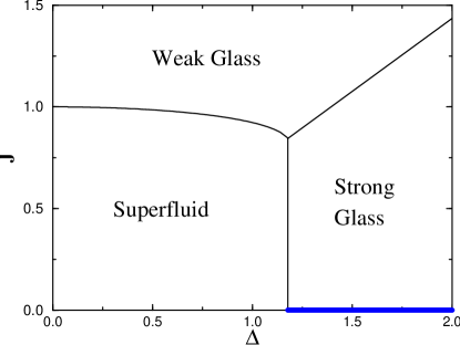
FIG. 1.: The $r=2$ phase diagram at T=0; parameters in units of $J_{0}$. The heavy line on the $\Delta$ axis is the Bose Glass.

As the superfluid state remains separated from the glassy continuum by a gap, just as in the clean case, it is obvious that the transition into it stays mean field like as well[10]. Therefore in the rest of the paper we set $J_{0}=0$ (also allowing to set $J=1$) and concentrate on the different spin-glass transitions. We explore the difference between these two glassy regimes by calculating the participation ratio $P$[10] of the Weak Glass state with the help of the cavity method[12]. In this approach a single site $i$ is isolated, then the magnetization $m_{j}$ at some other site $j$ is given as the magnetization of the site in the absence of site $i$, $m_{j}^{i}$, plus the effective field from $i$ times the local susceptibility $\sigma_{j}$: $m_{j}~{}=~{}m_{j}^{i}+\sigma_{j}~{}J_{ji}~{}m_{i}~{}~{}.$ Using this form in the eigenvalue equation for $H$, the magnetization is obtained self-consistently. We obtain for $P^{-1}=\sum_{i}m_{i}^{4}~{}$: $~{}(N/P)=\langle({\tilde{\omega}}_{WG}-h-\sigma({\tilde{\omega}}_{WG}))^{-4}\rangle_{h}$. The participation ratio for $r=2$, as plotted in the insert of Fig.2. clearly exhibits an extended Weak Glass state for weak disorder, which gets localized at the same $\Delta_{c}$ at which the Weak Glass state is absorbed into the continuum.

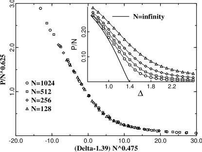
FIG. 2.: Scaling plot of the participation ratio.

The localization of the edge state of the continuum has a dramatic effect on the critical behaviour of the non-linear susceptibility: $\chi_{nl}^{-1}\sim 1-\langle\sigma_{i}^{2}\rangle_{h}$ [13]. As seen from Eq.(4), for the Weak Glass state $1-\langle\sigma_{i}^{2}\rangle_{h}=0$, i.e. $\chi_{nl}$ appropriately diverges when $\mu$ approaches the edge of the band at $\omega_{WG}$ (in fact with a $1/2$ exponent)[14]. For the Strong Glass state Eq.(4) does not hold anymore, leading to the striking result that $\chi_{nl}$ is finite at this glass transition.

We can also compute the ground state eigenvector of $H$ numerically. Treating the participation ratio as a generalized susceptibility suggests the scaling form: $P=N^{1-\eta}f\bigl{(}(\Delta-\Delta_{c})N^{1/{\tilde{\nu}}}\bigr{)}$, where $f(x)$ is a universal scaling function for a fixed $r$. The collapse of the curves for several system sizes in Fig.2. is a reliable verification of this scaling assumption. In the fitting procedure we used the theoretical value of $\Delta_{c}=[27/4\ln(4/3)]^{1/2}=1.393$. The exponents were then determined as: $\eta=0.37\pm 0.01$ and ${\tilde{\nu}}=2.10\pm 0.10$. Both exponents describe the scaling of spatial correlations with the finite system size. As our analytic technique was conceived for $N=\infty$, presently the determination of their value is beyond the scope of this work. The one combination which can be contrasted with our calculation is their product, appearing in the form: $P/N\sim(\Delta_{c}-\Delta)^{\eta{\tilde{\nu}}}$. The numerical procedure gives $\eta{\tilde{\nu}}=0.79$, whereas analytically we get an $\sim x/\ln~{}x$ asymptotics, which are numerically indistinguishable.

So far we considered the limit of vanishing concentration of holes in the Mott phase. Upon decreasing the chemical potential $\mu$ a finite concentration of holes appears and a genuinely many-body treatment becomes necessary. The usual replica trick is employed, leading to the free energy $F=lim_{n\rightarrow 0}f_{n}/n$, where:

$$f_{n} = {1\over 2}Tr~{}{\bf Q}^{2}-{1\over N}\sum_{i}~{}\ln~{}\Phi_{i}$$ (5)

$$\Phi_{i} = Tr~{}e^{-\beta H_{i}^{0}}T_{\tau}\exp[{\bf a^{\dagger}Qa}]$$ (6)

Here the elements of the vector of annihilation operators ${\bf a}$ are indexed as $a_{\alpha}(\tau)$, and that of the matrix ${\bf Q}$ as $Q_{\alpha\beta}(\tau,\tau^{\prime})$. The matrix product implies a summation over the replica indices and an integration over the time variables. Also, $H_{i}^{0}=-\mu_{i}\sum_{\alpha}a_{\alpha}^{\dagger}a_{\alpha}$ and $T_{\tau}$ denotes the time ordering operator. In these equations ${\bf Q}$ satisfies the saddle-point condition:

$$Q_{\alpha\beta}(\tau,\tau^{\prime})={1\over N}\sum_{i}\bigl{\langle}T_{\tau}a_{\alpha}^{\dagger}(\tau)a_{\beta}(\tau^{\prime})\bigr{\rangle}_{\Phi_{i}}~{},$$ (7)

where ${\langle\cdots\rangle}_{\Phi_{i}}$ indicates averaging with respect to ${\Phi_{i}}$.

Here we introduce the key technical step of our work: a coherent path integral representation for the boson operators as follows:

$$e^{{\bf a^{\dagger}Qa}}=\int{D{\bf\varphi}^{*}D{\bf\varphi}\over Det{\bf Q}}\exp[-{\bf\varphi^{*}Q^{-1}\varphi+\varphi a^{\dagger}+\varphi^{*}a}]$$ (8)

With the help of these new field operators the self-consistent equation for $Q$ transforms into:

$${\bf Q}(i\omega_{n}) = {1\over N}\sum_{i}\Bigl{[}{\bf E_{i}}(i\omega_{n})-{\bf Q}(i\omega_{n})\Bigr{]}^{-1}$$ (9)

$${\bf E_{i}}(i\omega_{n}) = [{\bf g^{o}_{i}}(i\omega_{n})-{\bf\Sigma}_{i}(i\omega_{n})]^{-1}~{}~{}~{}$$ (10)

As the Fourier transforms of all matrices are diagonal in frequency, from now on these remain matrices in the replica space only. Here ${\bf[g^{o}_{i}}]^{-1}(i\omega_{n})=(i\omega_{n}+\mu_{i})\delta_{\alpha\beta}$ is the on-site hole Green’s function at site $i$. ${\bf\Sigma}_{i}(i\omega_{n})$ is the self energy of the Green’s function: $G_{i}(i\omega_{n})_{\alpha\beta}=\langle\varphi^{*}_{\alpha}(i\omega_{n})\varphi_{\beta}(i\omega_{n})\rangle_{S_{i}}$, with the local action:

$$S_{i}=-{\bf\varphi^{*}Q^{-1}\varphi}+\ln Tre^{-\beta H_{i}^{0}}T_{\tau}e^{\bf\varphi a^{\dagger}+\varphi^{*}a}~{}~{}.$$ (11)

We expand the action $S_{i}$ up to fourth order, generating an effective $\varphi^{4}$ theory. Using this form one can construct a perturbative expansion for the Green’s function in order to determine the self energy ${\bf\Sigma}_{i}(i\omega_{n})$. For now we stop at the level of the fully dressed Hartree diagram, which yields a replica diagonal self-energy. In the absence of off-diagonal elements in the self energy it is reasonable to proceed with a replica symmetric form for ${\bf Q}$: $Q_{\alpha\beta}(i\omega_{n})=\delta_{\alpha\beta}\sigma(i\omega_{n})+\delta(i\omega_{n})\beta q$. Substituting this form for ${\bf Q}$ in Eq.(9) determines the parameters as:

$$\sigma(i\omega_{n}) = {1\over N}\sum_{i}{1\over E_{i}(i\omega_{n})-\sigma(i\omega_{n})}$$ (12)

$$q = {q\over N}\sum_{i}{1\over(E_{i}(0)-\sigma(0))^{2}}$$ (13)

We summarize the solutions of these equations at $T=0$. In the disordered phase, characterized by $q=0$, the self energy ${\bf\Sigma_{i}}(i\omega_{n})$ vanishes exponentially with T because of the presence of the gap. In the dilute limit, after appropriate transformations, these equations are identical with Eq.(2).

The Weak Glass phase is easiest understood by noticing that all formulae can in fact be expanded in the on-site disorder strength around $\Delta=0$. In this case one finds $E=2,~{}~{}\sigma(0)=1$ and $\Sigma(0)\sim q\sim(\mu_{c}-\mu)$. Concerning the spectrum, at low frequencies $E(i\omega_{n})=2+const.\times(i\omega_{n})$, reproducing the frequency dependence of Eq.(2); i.e. the spectrum again starts with a square root form at low energies, just as at the critical point, as determined in the one-particle picture. Thus the Mott-to-Weak Glass transition is completely mean-field in character. In other words, the global order parameter $q$ in Eq.(13) is generated by comparable contributions from all sites, indicating that the transition is driven by long range spatial correlations.

The physics of the Strong Glass transition is profoundly different. As the chemical potential is lowered, on the right hand side (rhs.) of Eq.(13), a few sites develop singular contributions. These local instabilities have to be regulated by generating a non-zero value for $q$. Obviously it is impossible to expand the rhs. around these singular points. This non-analyticity is well demonstrated in the rather non-traditional scenario for the transition: even at the transition the coefficient of $q$ on the rhs. of Eq.(13) is less than one (since here ${\bf E_{i}=\mu_{i}}$, hence it becomes equal to $\langle\sigma_{i}^{2}\rangle_{h}$, which is less than one outside the Weak Glass phase). On the other hand, inside the glass phase (where $q>0$) the coefficient of $q$ must equal unity, therefore it jumps at the transition. This profound non-analyticity signals a genuinely new type of transition, which is driven by local instabilities.

Next we extract the critical behaviour of $q$. There are three types of terms to the denominator $E_{i}(0)-\sigma(0)$ in Eq.(10). Sites with energies larger than $\sigma(0)$ give non-singular contributions $\mu_{i}+const.\times q$ just as for the Weak Glass. Sites with energies sufficiently below $\sigma(0)$ contribute $\sim q^{1/2}$, whereas sites close to $\sigma(0)$ yield $\sim q^{1/3}$. Taking into account the width of these last two integration regions gives $q\sim(\mu_{c}-\mu)^{4}$, with the subleading contribution $\sim(\mu_{c}-\mu)^{6}$. The spectrum is computed by expanding the denominator for small frequencies. One gets $Im\sigma\sim\omega^{1/2}$. The spectrum is quadratic in the Mott phase and even at the transition, i.e. the discontinuity in $q$’s coefficient in Eq. (13) translates into a jump in the spectrum exponent, but the behaviour of $q$ remains continuous, see Fig.3. Again, the exponents of the Strong Glass criticality depend on $r$.

FIG. 3.: The DOS in the Strong Glass region ($\Delta=2.0$, for which $\mu_{c}=2.589$).

The following “phase diagram” emerges from these considerations. The transitions into the Weak and Strong Glass regions from the Mott phase are characterized by different exponents. The same is true approaching these boundaries from inside the glassy phases, however these two glasses do not possess different order parameters, hence they are not distinct phases in the thermodynamic sense. The spin glass order parameter $q$ is non-zero in both, and the spectrum starts with a square root form in both as well.

When crossing from the Weak to the Strong Glass, the magnitude of $q$ is a reliable indicator, as its value drops by orders of magnitude (see Fig.3). This is so because its asymptotic exponent of four is strongly different from the mean field value of one. This gives rise to an anomalously large critical region - the Strong Glass -, which is dominated by the local fluctuations, severely suppressing the value of $q$. When approaching from the Mott phase, the non-linear susceptibility does not diverge, neither does $q$ develop an appreciable magnitude. Here the best indicator is the low frequency spectrum. The Mott gap shrinks to zero at the transition. Entering the Strong Glass the decreasing chemical potential shifts the spectral weight further down. To accomodate this weight at low positive frequencies, the spectrum has to bulge up, taking a square root form: $\sim(\mu_{c}-\mu)\times\omega^{1/2}$, giving way to a shifted quadratic form only at higher frequencies (Fig.3). Thus measuring the DOS at a low fixed frequency exhibits a gap in the Mott phase, and a roughly linearly increasing value inside the Strong Glass.

Lastly we comment on the issue of replica symmetry breaking. By explicit construction we can show that the replica symmetric solution is self-consistent in the Hartree approximation. Inspection of the structure of the higher order diagrams reveals that if the replica symmetry is broken, the degree of this is at most proportional to the temperature, thus vanishing at $T=0$.

In sum, we developed a theory for the quantum vortex glass, closely related to XY magnets and bosons in disodered media. We included disorder both for the coupling strengths and for the site energies. Utilizing one particle, many body and numerical methods we determined the phase diagram and the critical behaviour. We found a superfluid phase and Weak and Strong Glass regions, the physics of which is dominated by long range and local fluctuations, respectively. It was possible to go beyond previous approaches in the strongly disordered regime by introducing a coherent field representation for the hard core bosons. The most accessible experimental manifestation of the Strong Glass transition is the lack of divergence in the corresponding non-linear susceptibility. Analogous experimental findings have been reported in quantum spin-glass and vortex systems.

We acknowledge useful discussions with S. Sachdev. This work has been supported by NSF-DMR-95-28535.

REFERENCES

- [1] D.S. Fisher, Phys. Rev. Lett. 69, 534 (1993).
- [2] A.J. Bray and M.A. Moore, J. Phys. C 13, L655 (1980); Y.Y. Goldschmidt and P.Y. Lai, Phys. Rev. Lett. 64, 2567 (1990).
- [3] J. Miller and D. Huse, Phys. Rev. Lett. 70, 3147 (1993).
- [4] J. Ye, S. Sachdev and N. Read, Phys. Rev. Lett. 70, 4011 (1993); Phys. Rev. B. 52, 384 (1995).
- [5] M.P.A. Fisher, P.B. Weichman, G. Grinstein, and D.S. Fisher, Phys. Rev. B 40, 546 (1989).
- [6] W. Wu, D. Bitko, T.F. Rosenbaum and G. Aeppli, Phys. Rev. Lett. 71, 1919 (1993)
- [7] M. Guo, R.N. Bhatt and D.A. Huse, Phys. Rev. Lett. 72, 4137 (1994); H. Rieger and A.P. Young, ibid. 72, 4141 (1994).
- [8] C. Ebner and D. Stroud, Phys. Rev. B 31, 165 (1985).
- [9] T. Giamarchi and P. Le Doussal, Phys. Rev. Lett. 72, 1530 (1994).
- [10] F. Pázmándi, G.T. Zimanyi and R.T. Scalettar, Phys. Rev. Lett. 75, 1356 (1995).
- [11] E. Wigner Ann. Math. 65, 203 (1957).
- [12] M. Mezard, G. Parisi and M. Virasoro, Spin glass theory and beyond, World Scientific, Singapore, p.65 (1987).
- [13] T. Yamamoto and H. Ishii, J. Phys. C 20, 6053 (1987).
- [14] F. Pázmándi and Z. Domański, Phys. Rev. Lett. 74, 2363 (1995).