Long-range correlations and generic scale invariance in classical fluids
and disordered electron systems

Abstract

Long-ranged, or power-law, behavior of correlation functions in both space and time is discussed for classical systems and for quantum systems at finite temperature, and is compared with the corresponding behavior in quantum systems at zero temperature. The origin of the long-ranged correlations is explained in terms of soft modes. In general, correlations at zero temperature are of longer range than their finite temperature or classical counterparts. This phenomenon is due to additional soft modes that exist at zero temperature.

]

I Introduction

Homogeneous functions, or power laws, of space and time do not contain any intrinsic length or time scales, in contrast to, e.g., exponentials. This so-called scale invariance is well known to occur at critical points, where the critical modes become soft, which leads to power-law correlation functions.[1] Critical points are exceptional points in the phase diagrams of materials, and reaching them requires the fine tuning of parameter values. What is less well appreciated is the fact that many systems display what is now known as generic scale invariance (GSI), that is, power-law correlation functions in large regions of parameter space, with no fine tuning required at all to see them. GSI is due to soft modes that are not related to critical phenomena, but rather are due to conservation laws, or are otherwise inherent to the system. In recent years there has been a lot of attention paid to GSI, and the phenomenon has been discussed in a wide variety of systems, ranging from classical fluids and liquid crystals to disordered electrons and sandpiles. For recent reviews see Refs. [2].

In this paper we compare and contrast GSI and related phenomena in classical fluids and Lorentz gases with what we will call quantum GSI (QGSI), a similar but in general stronger effect that occurs in quantum systems at zero temperature. We will discuss four closely related topics: (1) The non-existence of virial expansions for the transport coefficients, (2) long-time tails, i.e. power-law decays of equilibrium time correlation functions that determine the transport coefficients, (3) long-range, or power-law, spatial correlations in non-equilibrium steady states, and (4) power-law spatial correlations in quantum mechanical systems in and out of equilibrium.

In Sec. II of this paper we review the occurrence of the above phenomena in classical fluids and Lorentz gases. In Sec. III we discuss the analogous effects in a quantum system, namely disordered electrons. In general, QGSI is characterized by correlations of longer range in space and/or time than those characteristic of the classical GSI. Reasons for this are discussed. In Sec. IV we conclude with a summary and a few remarks.

II Review of Classical Systems

A Density expansion of the transport coefficients

The first indications for long-ranged dynamical correlations in classical fluids appeared in the 1960’s, when problems were encountered in attempts to theoretically establish the density dependence of the transport coefficients of moderately dense gases. Up to that time it had been assumed that, in analogy with the virial expansion for the thermodynamic quantities[3] such as, e.g., the pressure, an analytic density expansion existed for an arbitrary transport coefficient, $\eta$, of the form,

$$\eta/\eta_{B}=1+a_{1,\eta}\,n^{*}+a_{2,\eta}\,(n^{*})^{2}+O\left((n^{*})^{3}\right)\quad.$$ (1)

Here $\eta_{B}$ is the Boltzmann value for $\eta$, which is exact in the limit of vanishing fluid density, $n\rightarrow 0$. $n^{*}=n\sigma^{d}$ is the reduced density, with $\sigma$ a molecular length scale and $d$ the spatial dimensionality of the system. The numbers $a_{l,\eta}$ are the coefficients in the virial expansion of $\eta$.

A density expansion of the form of Eq. (1) was predicted by Bogoliubov’s theory,[4] an extension and generalization of Boltzmann’s kinetic theory to higher densities. This theory was generally accepted at the time, and it gave the coefficients $a_{l,\eta}$ in terms of formally exact integrals. It came as a big surprise when a detailed analysis of these integrals showed that $a_{l,\eta}$ diverges for $l\geq 1$ in two-dimensional ($2$-$d$) systems, and for $l\geq 2$ in $3$-$d$ systems.[5] Shortly after this discovery, exact calculations for a model fluid, the classical Lorentz gas, confirmed these results.[6] A Lorentz gas consists of noninteracting particles that move in an array of randomly positioned, static hard disk ($d=2$) or hard sphere ($d=3$) scatterers.[7] The moving particles can be either classical or quantum in nature. The only relevant transport coefficient is the diffusion coefficient, or, equivalently, the particle mobility or conductivity. The important point was that the exact explicit calculations for classical Lorentz gases showed that the coefficients $a_{l,D}$ in the virial expansion, Eq. (1), for the diffusion coefficient are indeed divergent for $l\geq l^{*}$, and that the value of $l^{*}$ displays the dimensionality dependence suggested by the estimates for real gases. For later reference, we mention that the quantum version of the Lorentz gas is essentially the standard Edwards model for systems of disordered, noninteracting electrons.[8]

These divergencies in the virial coefficients are a clear indication of the presence of long-ranged dynamical correlations in both Lorentz gases and real gases. They have the following origin: In making a virial expansion, one assumes that the $l$-th term in Eq. (1) is determined by the dynamics of a cluster of $l+2$ particles moving in the infinite system. Because the cluster is considered in isolation, the $l+2$ particles can travel over arbitrarily large distances between collisions. However, this can occur neither in a real gas nor in a Lorentz gas, since the presence of the other particles that are not members of the cluster under consideration means that a particle cannot travel farther than a distance on the order of a mean-free path before it collides with another particle. This is a collective many-particle effect that was missed in Bogoliubov’s cluster expansion. Its existence precludes a virial expansion for transport coefficients. Mathematically, this physical effect leads to a nonanalytic density dependence of the transport coefficients, i.e. the virial coefficients are not simply numbers, but nonanalytic functions of the density. The leading nonanalyticity turns out to be logarithmic,[9] in agreement with the logarithmic divergence found in the early work. Equation (1) then takes the form, in $d=3$,

$$\eta/\eta_{B}=1+a_{1,\eta}\,n^{*}+{a^{\prime}}_{2,\eta}\,(n^{*})^{2}\log n^{*}+a_{2,\eta}\,(n^{*})^{2}$$ (2)

$$+\ o\left((n^{*})^{2}\right)\quad.$$ (3)

Here $o\left((n^{*})^{2}\right)$ denotes a term that for $n^{*}\rightarrow 0$ vanishes faster than $(n^{*})^{2}$. For real gases, only estimates of the coefficient ${a^{\prime}}_{2,\eta}$ are known.[10] For the classical Lorentz gas, ${a^{\prime}}_{2,D}$ is known exactly.[6]

B Long-time tails

Up until the late 1960’s it was also thought that the equilibrium time correlation functions that determine the transport coefficients decay exponentially with time for long times. This belief was based again on Bogoliubov’s kinetic theory, which predicted such an exponential decay. Actually, the separation of time scales that is present only with exponentially decaying time correlations was an important presumption in that theory. This appeared to be very plausible since the Boltzmann equation, which becomes exact in the limit of dilute gases, also yields an exponential decay of time correlations, which seemed to guarantee an exponential decay at least for dilute gases. It was therefore a further completely unexpected development when Alder and Wainwright,[11] in a computer study of self-diffusion in systems of hard disks and hard spheres, discovered that the equilibrium velocity autocorrelation function, $\langle{\bf v}(0)\cdot{\bf v}(t)\rangle_{\rm eq}$, whose time integral determines the diffusion coefficient, $D$, via

$$D={1\over d}\int_{0}^{\infty}dt\ \langle{\bf v}(0)\cdot{\bf v}(t)\rangle_{\rm eq}\quad,$$ (4)

decays only algebraically with time, namely,

$$\langle{\bf v}(0)\cdot{\bf v}(t)\rangle_{\rm eq}\approx c\,(t_{0}/t)^{d/2}\quad({\rm for}\quad t>>t_{0})\quad,$$ (5)

where $t_{0}$ is the mean-free time between collisions. Here $<\ldots>_{\rm eq}$ denotes an equilibrium thermal average. This slow decay of correlation functions is known as a long-time tail (LTT). The constant $c$ is positive, which implies that the LTT contribution to the autocorrelation function increases the diffusion rate compared to the Boltzmann result. Note that Eqs. (4) and (5) imply that the diffusion coefficient $D$ does not exist for $d\leq 2$, and that for low frequencies, the frequency dependent diffusion coefficient, $D(\omega)$, behaves as,

$$D(\omega)/D_{0}=1-c^{\prime}\,(i\omega)^{(d-2)/2}+\ldots\quad(d>2)\quad,$$ (7)

$$D(\omega)/D_{0}=1-c^{\prime\prime}\,\log(i\omega)+\ldots\quad(d=2)\quad,$$ (8)

with $D_{0}$ the static or zero-frequency diffusion coefficient, and $c^{\prime}$ and $c^{\prime\prime}$ positive constants.

Equation (5) was later derived theoretically by Ernst, Hauge, and van Leeuwen,[12] and by Dorfman and Cohen.[13] The basic physical idea behind the explanation of the LTT phenomena is that it is the hydrodynamic processes that determine the long-time behavior of all correlation functions. Of particular importance are recollision processes, where after a collision, the two involved particles diffuse away and then come back and recollide. We can see this in Eq. (5), the right-hand side of which is proportional to the probability that a diffusing particle returns at time $t$ to the point it started out from at $t=0$. This concept is a very general one, and it turns out that all of the transport coefficients in a classical fluid have LTT like those shown in Eqs. (5) and (5). That is, if $\eta(\omega)$ is a general frequency dependent transport coefficient, then

$$\eta(\omega)/{\eta}_{0}=1-c_{\eta}^{\prime}\,(i\omega)^{(d-2)/2}+\ldots\quad(d>2)\quad,$$ (10)

$$\eta(\omega)/{\eta}_{0}=1-c_{\eta}^{\prime\prime}\,\log(i\omega)+\ldots\quad(d=2)\quad.$$ (11)

The existence of LTT even for arbitrarily dilute fluids is not in contradiction with the Boltzmann equation becoming exact in the dilute limit. The point is that the Boltzmann equation becomes exact for fixed time in the limit of vanishing density, but not for fixed density, no matter how small, in the limit of long times. The way the dilute limit is reached is that with decreasing density, one has to go to longer and longer times in order to see the LTT, and the preasymptotic decay is well described by the Boltzmann equation.

It was pointed out above that the LTT in a fluid are related to the probability of a diffusing particle to return at time $t$ to the point where it was at time $t=0$. Although the recollision events that are responsible for this return probability always occur, this does not necessarily imply that all correlation functions in a given system (other than a real classical fluid) decay as $t^{-d/2}$. Rather, it just suggests the possibility that they do, and whether or not a particular correlation function actually does so, depends on whether the corresponding observable couples sufficiently strongly to the hydrodynamic processes in the system under consideration. It is plausible to assume that, for any given observable, coupling to the diffusion process is more likely the more hydrodynamic or soft modes there are in the system. For example, in a $d$-dimensional real fluid there are $d+2$ soft modes due to the $d+2$ conservation laws for particle number, energy, and momentum. In contrast, in a Lorentz gas only particle number (and, trivially, energy) is conserved. This smaller number of hydrodynamic modes suggests, according to the above argument, that the LTT might be weaker in a Lorentz gas than in a real fluid. Indeed, the velocity autocorrelation function in a Lorentz gas decays as,[14]

$$\langle{\bf v}(0)\cdot{\bf v}(t)\rangle_{\rm eq}\approx-c\,(t_{0}/t)^{(d+2)/2}\quad({\rm for}\quad t>>t_{0})\quad,$$ (12)

and the frequency dependent diffusion coefficient is given by

$$D(\omega)/D_{0}=1+a\,i\omega+b\,(i\omega)^{d/2}+\ldots\quad(d>2)\quad,$$ (14)

$$D(\omega)/D_{0}=1+b^{\prime}\,i\omega\,\log(i\omega)+\ldots\quad(d=2)\quad.$$ (15)

The coefficients $c$, $b$, and $b^{\prime}$ in Eqs. (12) and (12) are positive. This sign occurs because in a Lorentz gas, in contrast to a real fluid, any recollision process decreases the diffusion rate. This is a consequence of the missing dynamics of the scatterers.

C Long-range correlations in nonequilibrium steady states

In contrast to the slow time decay of equilibrium time correlation functions for classical fluids discussed in the last subsection, the spatial correlations decay exponentially in such systems, except at isolated critical points. This asymmetry between space and time correlations is related to the detailed balance relation that is valid in equilibrium, and it is not generic. In more general states, e.g. in nonequilibrium steady states, where detailed balance is absent and where there is spatial anisotropy, long-range correlations occur in both space and time.[15]

From a general point of view the existence of long-ranged spatial correlations is not surprising. Thermal fluctuations constantly appear in a fluid, and then decay. Their behavior at long distances is determined by the soft dynamical modes that are singular in the long-wavelength limit. For example, in the static or zero-frequency limit, the diffusion equation becomes Laplace’s equation whose solution exhibits a power-law decay in space.

The best studied system, both theoretically and experimentally, is a simple fluid subject to a stationary temperature gradient.[15, 16] Using light scattering, the Fourier transform of the density autocorrelation function,

$$S({\bf x},{\bf x}^{\prime})=\langle\delta n({\bf x})\ \delta n({\bf x}^{\prime})\rangle\quad,$$ (16)

can be measured. Here $\delta n({\bf x})$ is a density fluctuation at point ${\bf x}$, and the angular brackets denote a nonequilibrium ensemble average. Theoretically, both microscopic many-body techniques and more phenomenological approaches yield,[17]

$$S({\bf k})=S_{0}\,\left[1+\left({{\hat{\bf k}}_{\perp}\cdot\nabla T\over{\bf k}^{2}}\right)^{2}\ {c_{p}\over T\,D_{T}(\nu+D_{T})}\right]\quad.$$ (17)

Here ${\bf k}$ is the wavevector, $c_{p}$ is the specific heat at constant pressure, $D_{T}$ is the thermal diffusion coefficient, $\nu$ is the kinematic viscosity, ${\hat{\bf k}}_{\perp}$ is a unit vector perpendicular to ${\bf k}$, and $S_{0}$ is the equilibrium static structure factor that is $k$-independent in the long wavelength limit. Equation (17) for $S({\bf k})$ is well confirmed experimentally. For the implications of Eq. (17) in real space, see Ref. [18].

Theoretically, long-range correlations in a nonequilibrium Lorentz gas have also been studied. The system considered is a Lorentz gas in the presence of a chemical potential gradient, $\nabla\mu$. As mentioned earlier, the only soft mode in this model is the diffusive number density. Because the diffusing particles in a Lorentz model do not interact, correlations can only occur between the moving particles and the scatterers. Denoting the density fluctuations of the former by $\delta n({\bf x})$, and the scatterer density for a given configuration by $N({\bf x})$, a measure of this correlation is the particle-scatterer density correlation,

$$S({\bf x},{\bf x}^{\prime})=\langle\delta n({\bf x})\,N({\bf x}^{\prime})\rangle\quad.$$ (18)

In Fourier space, a kinetic theory calculation yields,[19]

$$S({\bf k})={i{\bf k}\cdot\nabla\mu\over 2\pi D{\bf k}^{2}}\quad,$$ (19)

with $D$ the diffusion coefficient. In real space, Eq. (19) implies that $S(r)$ decays like $r^{1-d}$. Again, the correlations are stronger in the real fluid than in the Lorentz gas.

III Disordered Electrons at Zero Temperature

A Density expansion of the electron mobility

In disordered electronic systems, there are two length scales that can be used to construct a dimensionless small parameter from the scatterer density $n$, namely the scattering length $\sigma$ and the Fermi wavelength $\lambda_{F}=2\pi/k_{F}$. We can thus form the dimensionless densities (for $d=3$) $n\lambda_{F}^{3}$, $n\lambda_{F}^{2}\sigma$, $n\lambda_{F}\sigma^{2}$, and $n\sigma^{3}$. The first two do not appear in the standard perturbation theory that expands in powers of $n$.[8] The third one is usually written as $1/k_{F}l\equiv\epsilon$, with $l\sim 1/n\sigma^{2}$ the mean-free path. The fourth one is the quantity $n^{*}=n\sigma^{3}$ that also has a classical meaning. Now consider a dilute electron system in the sense that $\lambda_{F}>>\sigma$. In that case we have $n^{*}\sim\sigma/l<<\epsilon$, and hence $n^{*}$ can be neglected compared to $\epsilon$. Notice that in the quantum Lorentz gas, the dilute limit needs to be considered even for noninteracting quantum particles, since the Pauli principle establishes correlations, and hence an effective interaction, between the particles.

For dimensions $d>2$, the system is diffusive as long as $\epsilon<\epsilon^{*}$, with $\epsilon^{*}=O(1)$ for $d=3$. At $\epsilon=\epsilon^{*}$ a metal-insulator transition called the Anderson transition takes place.[20] For dilute systems in the above sense, $n^{*}<<1$ even at the Anderson transition, and the latter is well separated from the percolation transition that would occur at $n^{*}\approx 1$.

Considering the generalized virial expansion given by Eq. (3) it is natural to ask whether or not a similar expression holds for a quantum Lorentz gas with the parameter $\epsilon$ defined above replacing the classical reduced density $n^{*}$. This question was first asked, and answered affirmatively, as early as 1966.[21] More recently, all of the terms in the expansion up to and including those of $O(\epsilon^{2})$ have been computed exactly.[22] In order to compare the resulting expression with real experimental data, the electron mobility, $\mu$, of electrons injected into Helium gas at low temperatures has been considered. Because the Helium atoms are very massive compared to the electrons, the quantum Lorentz gas constitutes an excellent model for this system. Furthermore, there is experimental control over the density of the injected electrons, which means that the abovementioned diluteness condition can be fulfilled to an extremely high degree. This also means that Coulomb interaction effects can be made negligible. In order to model the actual experimental situation, one needs to consider a nondegenerate gas of electrons at temperature $T$ with the thermal de Broglie wavelength, $\lambda_{T}=2\pi/k_{T}=(2\pi/mk_{B}T)^{1/2}$, replacing $\lambda_{F}$ in $\epsilon$. Defining $\chi=2/k_{T}l$, an exact calculation gives,[22]

$$\mu/\mu_{\rm cl}=1+\mu_{1}\,\chi+{\mu}^{\prime}_{2}\,\chi^{2}\log\chi+\mu_{2}\,\chi^{2}+o\left(\chi^{2}\right)\quad,$$ (21)

with

$$\mu_{1}=-\pi^{3/2}/6\quad\quad,$$ (22)

$${\mu}^{\prime}_{2}=\left(\pi^{2}-4\right)/32\quad,$$ (23)

$$\mu_{2}=0.236\ldots\quad\quad,$$ (24)

and $\mu_{\rm cl}$ the classical or Boltzmann value for the mobility.

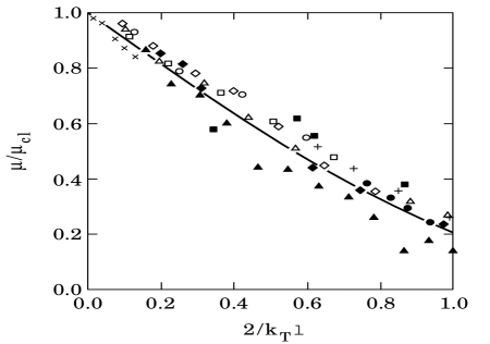
FIG. 1.: Mobility $\mu$ of electrons in dense gases, normalized to the Boltzmann value $\mu_{\rm cl}$, as a function of $\chi$. The symbols represent experimental data, the solid line is the theoretical result, Eq. (21). After Ref. [23].

In Figs. 1 and 2 this theoretical result is compared with experimental data. Of particular interest is the question whether this kind of analysis can be used to experimentally confirm the existence of the logarithmic term in Eq. (21). In classical systems the corresponding logarithmic term in Eq. (3) has never been convincingly observed,[10] mostly due to the fact that the coefficients in the density expansion are not known exactly for any realistic classical system. The fact that the quantum Lorentz gas is such a good model for electrons in Helium gas makes this system a very promising one for attempts to finally observe the logarithm. As a measure of the logarithmic term, one defines,[22]

$$f(\chi)\equiv\left[\ \mu/\mu_{\rm cl}-1-\mu_{1}\,\chi\ \right]/\chi^{2}\quad.$$ (26)

The theoretical prediction for this quantity is,

$$f(\chi)={\mu}^{\prime}_{2}\,\log\chi+\mu_{2}\pm\mu_{2}\,2\sqrt{\pi}\chi\quad.$$ (27)

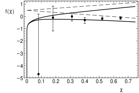
FIG. 2.: The reduced mobility $f$, as defined in Eq. (26), vs. the density parameter $\chi=2/k_{T}l$. The theoretical prediction is for $f$ to lie between the two solid lines. The experimental data are from Fig. 9 of Ref. [24] with error bars estimated as described in Ref. [22]. The broken lines show what the theoretical prediction would be in the absence of the logarithmic term in the density expansion. From Ref. [22].

The last term in Eq. (27) is an estimate of the effect of all higher order terms. At $T=4.2{\rm K}$, a Helium gas density of $n=10^{21}{\rm cm}^{-3}$ corresponds to $\chi=1$, and data were obtained for $\chi$ as small as $0.08$. Fig. 2 shows the theoretical prediction, Eq. (27), for $0<\chi<0.7$ together with data by Schwarz. We conclude that the existing experimental data are consistent with the theoretical result. However, for a convincing demonstration of the existence of the logarithmic term an improvement in the experimental accuracy by about a factor of ten over Schwarz’s experiment would be necessary.

B Long-time tails, a.k.a. weak localization effects

The results discussed in the previous subsection seems to suggest that there is no conceptual difference between transport in classical and dilute quantum Lorentz gases: The forms of the density or disorder expansions, Eqs. (3) and (III A), are identical, even though the dimensionless expansion parameters are different. This conclusion is fallacious, however, as can be seen by considering the LTT in the time correlation functions, or in the low frequency expansions of the transport coefficients for the two models. Here we first quote the quantum result, and then we discuss the reason for it being qualitatively different from its classical counterpart.

Any of a variety of theoretical methods leads to a frequency dependent electrical conductivity for a quantum Lorentz gas whose real part is of the form,[25, 26]

$$\sigma(\omega)/\sigma_{0}=1+c\,\omega^{(d-2)/2}+\ldots\quad({\rm for}\quad d>2)\quad,$$ (29)

$$\sigma(\omega)/\sigma_{0}=1+c^{\prime}\,\log\omega+\ldots\quad({\rm for}\quad d=2)\quad.$$ (30)

Equations (29), (30) imply that the current-current correlation function that is defined as the Fourier transform of the real part of the conductivity has a LTT,

$$\sigma(t)\approx-c\,(t_{0}/t)^{d/2}\quad({\rm for}\quad t>>t_{0})\quad.$$ (31)

The coefficient $c$ in Eq. (31) is positive. For $d=2$, and more generally for $d\leq 2$, the low frequency expansion of $\sigma(\omega)$ breaks down, and the static conductivity or the static diffusion coefficient is actually zero. That is, for $d\leq 2$ there is no metallic phase at zero temperature.[27, 20] At finite temperature and zero frequency, the temperature dependence of $\sigma$ is obtained by replacing the frequency in Eqs. (29) and (30) by the temperature $T$. For $T>0$ and $\omega\rightarrow 0$ the leading frequency dependences are given by Eqs. (12), i.e., the classical result is recovered. Figure 3 shows an example of the temperature dependent resistivity of a thin metallic film, which is logarithmic for low temperatures in agreement with the above remarks.

FIG. 3.: Resistance, $R$, normalized to $R_{0}=R(T=1K)$, of a thin PdAu film plotted versus $\log T$. After Ref. [28].

Let us now discuss the interesting difference between the frequency dependencies in Eqs. (12) and (III B). Equations (12) can be derived not only from a classical microscopic many-body approach, but also from a more general phenomenological approach that appears to be independent of whether or not the underlying description is classical or quantum mechanical.[29] The crucial assumption is that the only slow mode in the problem is due to particle number conservation. Remarkably, it is this assumption that breaks down in the quantum case, and this is what leads to the differences between Eqs. (12) and (III B). To understand this important point, let us consider a field theoretic description of a disordered fermion system,[30] that we assume to be noninteracting for simplicity. The partition function is,

$$Z=\int_{\psi(0)=-\psi(1/k_{B}T)}D[\bar{\psi},\psi]\ \exp\left(S[\bar{\psi},\psi]\right)\quad,$$ (33)

with the action $S$ given by,

$$S[\bar{\psi},\psi]=-\int dx\ \bar{\psi}(x)\,{\partial\over\partial\tau}\,\psi(x)+$$ (34)

$$+\int dx\ \bar{\psi}(x)\,\left[{\Delta\over 2m}+\mu-u({\bf x})\right]\,\psi(x)\quad.$$ (35)

Here we have used a four-vector notation, $x\equiv({\bf x},\tau)$, $\int dx\equiv\int d{\bf x}\,\int_{0}^{1/T}d\tau$, with $\tau$ denoting imaginary time. $m$ is the fermion mass, $\mu$ is the chemical potential, $u({\bf x})$ is a random potential, and for notational simplicity we have suppressed the spin labels. Since we are considering fermions, the fields $\bar{\psi}$ and $\psi$ are Grassmann valued and $D[\bar{\psi},\psi]$ is a Grassmannian functional integration measure, but for the following arguments this will not be crucial. By changing from imaginary time representation to a frequency representation,

$$\psi(x)=T^{1/2}\sum_{n}e^{-i\omega_{n}\tau}\,\psi_{n}({\bf x})\quad,$$ (37)

with Matsubara frequencies

$$\omega_{n}=2\pi T(n+1/2)\quad,\quad(n=0,\pm 1,\ldots)\quad,$$ (38)

the action can be written,

$$S=\sum_{n}\int d{\bf x}\ \bar{\psi}_{n}({\bf x})\,\left[{1\over 2m}\Delta+\mu-u({\bf x})-i\omega_{n}\right]\,\psi_{n}({\bf x})\quad.$$ (39)

The crucial point is that for $\omega_{n}=0$, or $T=0$, the action given by Eq. (39) is invariant under a unitary transformation of the fields in frequency space, $\psi_{n}\rightarrow\sum_{m}U_{nm}\psi_{m}$. In fact, $S$ is invariant under a larger symplectic group that also includes a time reversal symmetry, but we ignore this technical point here. We further note that the ‘order parameter’,

$$Q=\lim_{\omega_{n}\rightarrow 0+}\langle\bar{\psi}_{n}({\bf x})\,\psi_{n}({\bf x})\rangle-\lim_{\omega_{n}\rightarrow 0-}\langle\bar{\psi}_{n}({\bf x})\,\psi_{n}({\bf x})\rangle\quad,$$ (40)

is the single-particle spectral function, or the difference between the retarded and advanced Green functions. Because these functions have poles on opposite sides of the real axis, $Q$ is nonzero as long as the density of states at the Fermi surface is nonzero.

To use a magnetic analogy, having a nonzero $Q$ in Eq. (40) is similar to having a nonvanishing magnetization in the limit of a zero external field, and the abovementioned unitary symmetry is analogous to the rotational symmetry in spin space. This analogy implies that in the zero temperature fermion system there is a spontaneously broken continuous symmetry. This was first noticed in the context of the Anderson transition mentioned in Sec. III A.[31, 32] Goldstone’s theorem then implies that there are soft modes, namely particle-hole excitations, in addition to the ones implied by the conservation laws. Detailed calculations confirm that it is these additional soft modes that lead to the stronger LTT effects in Eqs. (III B) as compared to the classical LTT in Eqs. (12).

C Long-ranged spatial correlations in equilibrium

A characteristic feature of quantum statistical mechanics, as opposed to the classical theory, is the coupling of statics and dynamics. This can be seen in Eqs. (3), where the basic statistical field $\psi$ is a function of both space and imaginary time. As a result, one does not expect any qualitative differences between static and dynamic correlations even in equilibrium, in contrast to the asymmetry between these two types of correlations that is observed in classical systems and was discussed in Sec. II C above.

Indeed, a calculation of the wavenumber dependent static spin susceptibility, $\chi_{s}({\bf k})$, in a disordered system of interacting electrons yields the following behavior for small wavenumbers,[33, 34]

$$\chi_{s}({\bf k})=c_{0}-c_{d-2}\,|{\bf k}|^{d-2}-c_{2}\,{\bf k}^{2}+\ldots\quad,$$ (41)

where the $c_{i}$ are positive constants. In real space, the nonanalytic term proportional to $|{\bf k}|^{d-2}$, which for $d<4$ is the leading ${\bf k}$-dependence of $\chi_{s}$, corresponds to a long-range interaction between the electronic spin density fluctuations that falls off like $r^{2-2d}$. This has recently been shown to have interesting consequences for the ferromagnetic quantum phase transition that occurs in an itinerant electron system at zero temperature as a function of the exchange interaction.[34]

The origin of this long-range correlation can be traced back to the same Goldstone modes that were discussed in the last subsection, and that also lead to the LTT. In a disordered system, the Goldstone modes are diffusive, and give a contribution to the spin susceptibility that can be schematically represented by

$$\chi_{s}({\bf k})\sim\int_{k}^{\Lambda}dp\ p^{d-1}\int_{0}^{\infty}d\omega\ {\omega\over(D\,p^{2}+\omega)^{3}}\quad,$$ (42)

with $\Lambda$ an ultraviolet cutoff, and $D$ the spin diffusion coefficient. Equation (42) demonstrates the coupling of statics and dynamics that was mentioned above, and doing the integrals yields Eq. (41). The fact that this coupling is really a quantum effect can be seen by considering the corresponding expression at finite temperature. In this case one has to perform a frequency sum rather than an integral, and the net effect is that the term $|{\bf k}|^{d-2}$ in Eq. (41) is replaced by $({\bf k}^{2}+T)^{(d-2)/2}$. Hence, for $T>0$ an analytic expansion about ${\bf k}=0$ exists, and there are no long-ranged correlations.

D Long-ranged spatial correlations in nonequilibrium steady states

Very recently, spatial correlations of density fluctuations have been studied in noninteracting disordered electronic system that are not in equilibrium.[35] For the model defined by Eqs. (3) or (39) the correlation function analogous to Eq. (18) for the classical Lorentz gas is,

$$S_{1}({\bf x},{\bf x}^{\prime})=\left\{\langle\delta n({\bf x})\rangle\,u({\bf x}^{\prime})\right\}_{\rm dis}\quad,$$ (43)

where $\{\ldots\}_{\rm dis}$ denotes the disorder average, and $<\ldots>$ denotes a nonequilibrium thermal average as in Sec. II C. A direct many-body calculation shows that the Fourier transform of Eq. (43), $S_{1}({\bf k})$, behaves just like its classical counterpart, Eq. (19).

Because the moving particles are fermions, they effectively interact due to statistical correlations. As a measure of these correlations we consider the structure factor,

$$S_{2}({\bf x},{\bf x}^{\prime})=\left\{\langle\delta n({\bf x})\,\delta n({\bf x}^{\prime})\rangle\right\}_{\rm dis}\quad.$$ (44)

Let us consider the nonequilibrium part of $S_{2}$. For a classical, interacting, Lorentz gas one finds,

$$S_{2}({\bf k})\sim(\nabla\mu)^{2}/{\bf k}^{2}\quad.$$ (45)

Naively, one might anticipate a similar result for the disordered electron system at $T=0$. However, because of the additional soft modes that were discussed in the preceding section, the correlations here are much stronger, and the decay is much slower in space. A direct many-body calculation yields in the limit of small wavenumbers,

$$S_{2}({\bf k})={N_{F}\mu\tau\over 6d\pi(D{\bf k}^{2})^{2}}\,\left[25(\nabla\mu)^{2}-12({\hat{\bf k}}\cdot\nabla\mu)^{2}\right]\quad,$$ (46)

with $N_{f}$ the electronic density of states at the Fermi level, and $\tau$ the electronic mean-free time between collisions. In real space, Eq. (46) corresponds to a linear decay of $S_{2}(r)$ with distance.

IV Conclusion

In this paper we have reviewed classical and quantum versions of what one might call generalized long-time tail effects, that is long-range correlations in both space and time. We have seen that these effects are due to the hydrodynamic or soft modes in the system, which couple via mode-mode coupling effects to all other modes unless some symmetry prohibits such a coupling. Generally, the quantum or zero temperature versions of these effects are stronger, that is of longer range, than their classical counterparts, because of additional soft modes that exist at zero temperature. These additional soft modes are Goldstone modes that result from a broken symmetry in Matsubara frequency space, and are not related to conservation laws. Another additional effect in quantum systems is the coupling of statics and dynamics, which leads to both static and dynamic equilibrium correlations in general to be of long range, whereas in classical systems one has to consider nonequilibrium states in order to get long-ranged static correlations.

A phenomenon similar to the enhanced long-time tail effects in the quantum case is also known in certain classical systems with soft modes that are unrelated to conservation laws. For example, in the smectic-A phase of liquid crystals there are soft modes due to the conservation laws, and additional soft modes due to spontaneously broken symmetries and Goldstone’s theorem. The combination of these soft modes produce stronger long-time tail effects than are present in a simple classical fluid with no Goldstone modes.[36]

Finally, we mention that the effects in electronic systems discussed in Sec. III do not qualitatively hinge on the system being disordered. As can be seen from Eq. (39) and the related discussion, the broken symmetry argument still holds for clean electron fluids, with the only difference being that the Goldstone modes have a ballistic dispersion in that case, rather than a diffusive one. Consequently, the effects discussed in this paper qualitatively survive, only the various exponents change compared to the disordered system. These LTT effects in clean fermion systems can be related to known features of Fermi-liquid theory. This demonstrates the generality and unifying properties of the general physical approach taken in this paper.

- [1] See, e.g., S. K. Ma, Modern Theory of Critical Phenomena, (Benjamin, Reading, MA 1976); K. G. Wilson and J. Kogut, Phys. Rep. 12, 75 (1974).
- [2] See, e.g., B. M. Law and J. C. Nieuwoudt, Phys. Rev. A 40, 3880 (1989); J. R. Dorfman, T. R. Kirkpatrick, and J. V. Sengers, Ann. Rev. Phys. Chem. 45, 213 (1994); S. Nagel, Rev. Mod. Phys. 64, 321 (1992).
- [3] See, e.g., T. L. Hill, Statistical Mechanics, (Dover, New York 1987).
- [4] N. N. Bogoliubov, in Studies in Statistical Mechanics, Vol.I, eds. G. E. Uhlenbeck and J. de Boer (North-Holland, Amsterdam 1961), p.1.
- [5] J. R. Dorfman and E. G. D. Cohen, Phys. Lett. 16, 124 (1965); J. Math. Phys. 8, 282 (1967); J. Weinstock, Phys. Rev. 140A, 460 (1965). For further references see, e.g., J. R. Dorfman and H. van Beijeren in Statistical Mechanics, part B, edited by B. J. Berne, Plenum (New York 1977), p.65.
- [6] J. M. J. van Leeuwen and A. Weijland, Physica 36, 457 (1967); 38, 35 (1968).
- [7] For a discussion of Lorentz models, see, E. H. Hauge, in Transport Phenomena, Lecture Notes in Physics No. 31, edited by G. Kirczenow and J. Marro, Springer (New York 1974), p.337.
- [8] See, e.g., A. A. Abrikosov, L. P. Gorkov, and I. E. Dzyaloshinskii, Methods of Quantum Field Theory in Statistical Physics Prentice Hall (Englewood Cliffs, 1969), ch. 39; or G. D. Mahan Many-Particle Physics (Plenum Press, New York and London, 1981), ch. 7.
- [9] J. V. Sengers, Phys. Rev. Lett. 15,515 (1965); K. Kawasaki and I. Oppenheim, Phys. Rev. 139A, 1763 (1965); see also E. G. D. Cohen in Statistical Mechanics at the Turn of the Century, edited by E. G. D. Cohen, Marcel Dekker (New York 1971), p.33.
- [10] See, e.g., B. M. Law and J. V. Sengers, J. Stat. Phys. 57, 531 (1989).
- [11] B. J. Alder and T. E. Wainwright, Phys. Rev. Lett. 18, 988 (1967); J. Phys. Soc. Japan Suppl. 26, 267 (1968); Phys. Rev. A 1, 18 (1970).
- [12] M. H. Ernst, E. H. Hauge, and J. M. J. van Leeuwen, Phys. Rev. Lett. 25, 1254 (1970).
- [13] J. R. Dorfman and E. G. D. Cohen, Phys. Rev. Lett. 25, 1257 (1970).
- [14] M. H. Ernst and A. Weijland, Phys. Lett. 34A, 39 (1971).
- [15] See, e.g., J. R. Dorfman, T. R. Kirkpatrick, and J. V. Sengers, Ref. [2]
- [16] J. Weinstock, Phys. Rev. 140A, 460 (1965).
- [17] T. R. Kirkpatrick, E. G. D. Cohen, and J. R. Dorfman Phys. Rev. A 26, 995 (1982).
- [18] R. Schmitz, Phys. Rep. 171, 1 (1988).
- [19] M. Yoshimura and T. R. Kirkpatrick, Phys. Rev. E 52, 2676 (1995).
- [20] See, e.g., P. A. Lee and T. V. Ramakrishnan, Rev. Mod. Phys. 57, 287 (1985).
- [21] J. S. Langer and T. Neal, Phys. Rev. Lett. 16, 984 (1966); J. Weinstock, Phys. Rev. Lett. 17, 130 (1966); see also P. Resibois and M. G. Velarde, Physica 51, 541 (1971).
- [22] K. I. Wysokinski, W. Park, D. Belitz, and T. R. Kirkpatrick, Phys. Rev. Lett. 73, 2571 (1994); Phys. Rev. E 52, 612 (1995).
- [23] P. W. Adams, D. A. Browne, and M. A. Paalanen, Phys. Rev. B 45, 8837 (1992).
- [24] K. Schwarz, Phys. Rev. B 21, 5125 (1980).
- [25] L. P. Gorkov, A. I. Larkin, and D. E. Khmelnitskii, Pis’ma Zh. Teor. Eksp. Fiz. 30, 248 (1979) [JETP Lett. 30, 228 (1979)].
- [26] T. R. Kirkpatrick and J. R. Dorfman, Phys. Rev. A 28, 1022 (1983); J. Stat. Phys. 30, 67 (1983).
- [27] E. Abrahams, P. W. Anderson, D. C. Licciardello, and T. V. Ramakrishnan, Phys. Rev. Lett. 42, 673 (1979).
- [28] G. J. Dolan and D. D. Osheroff, Phys. Rev. Lett. 43, 721 (1979).
- [29] M. H. Ernst, J. Machta, H. van Beijeren, and J. R. Dorfman, J. Stat. Phys. 34, 477 (1984).
- [30] See, e.g., J. W. Negele and H. Orland, Quantum Many-Particle Systems (Addison-Wesley, New York 1988).
- [31] F. Wegner, Z. Phys. B 35, 207 (1979).
- [32] A. J. McKane and M. Stone, Ann. Phys. (NY) 131, 36 (1981).
- [33] T. R. Kirkpatrick and D. Belitz, Phys. Rev. B 41, 11082 (1990).
- [34] T. R. Kirkpatrick and D. Belitz, preprint (cond-mat/9601008).
- [35] M. Yoshimura and T. R. Kirkpatrick, preprint (cond-mat/96xxxxx).
- [36] G. F. Mazenko, S. Ramaswamy, and J. Toner, Phys. Rev. A 28, 1618 (1983).