Novel Symmetry Classes in Mesoscopic Normalconducting-Superconducting Hybrid Structures

Abstract

Normal-conducting mesoscopic systems in contact with a superconductor are classified by the symmetry operations of time reversal and rotation of the electron’s spin. Four symmetry classes are identified, which correspond to Cartan’s symmetric spaces of type $C$, $C$I, $D$, and $D$III. A detailed study is made of the systems where the phase shift due to Andreev reflection averages to zero along a typical semiclassical single-electron trajectory. Such systems are particularly interesting because they do not have a genuine excitation gap but support quasiparticle states close to the chemical potential. Disorder or dynamically generated chaos mixes the states and produces novel forms of universal level statistics. For two of the four universality classes, the $n$-level correlation functions are calculated by the mapping on a free 1D Fermi gas with a boundary. The remaining two classes are related to the Laguerre orthogonal and symplectic random-matrix ensembles. For a quantum dot with an NS-geometry, the weak localization correction to the conductance is calculated as a function of sticking probability and two perturbations breaking time-reversal symmetry and spin-rotation invariance. The universal conductance fluctuations are computed from a maximum-entropy $S$-matrix ensemble. They are larger by a factor of two than what is naively expected from the analogy with normal-conducting systems. This enhancement is explained by the doubling of the number of slow modes: owing to the coupling of particles and holes by the proximity to the superconductor, every cooperon and diffuson mode in the advanced-retarded channel entails a corresponding mode in the advanced-advanced (or retarded-retarded) channel.

74.80.Fp, 05.45.+b, 74.50.+r, 72.10.Bg

I Introduction

Following the early work of Wigner[1], Dyson in his classic 1962 paper[2] classified complex many-body systems such as atomic nuclei according to their fundamental symmetries. Arguing on mathematical grounds, he proposed the existence of three symmetry classes, which are distinguished by their behavior under reversal of the time direction and by their spin. The statistical properties of these classes are described by three random-matrix models, called the Gaussian Orthogonal, Unitary and Symplectic Ensembles (GOE, GUE, GSE). Dyson’s classification scheme has since proved very far reaching. Although atomic nuclei display only GOE statistics, physical realizations of the other two classes were later found in chaotic and disordered single-electron systems subject to a magnetic field (GUE) or to spin-orbit scattering (GSE).

By standard arguments, Wigner-Dyson statistics applies to the ergodic limit, i.e. to times long enough for the degrees of freedom to equilibrate and fill the available phase space uniformly. More specifically, in the context of disordered mesoscopic systems the ergodic limit is reached for times larger than the diffusion time $L^{2}/D$, where $D$ is the diffusion constant and $L$ the linear extension of the system. By the uncertainty relation, the ergodic limit corresponds to the energy range below the Thouless energy $\hbar D/L^{2}$.

One may ask whether the level statistics of disordered or chaotic single-particle systems in the ergodic limit must always be Wigner-Dyson or whether different statistics is possible. The answer is that Wigner-Dyson statistics is generic and universal as long as the statistics is required to be stationary under shifts of the energy. (This can be understood from the mapping on a nonlinear $\sigma$ model[3].) However, if the stationarity condition is relaxed and additional symmetries are imposed, new universality classes may arise. This happens, for instance, when a massless Dirac particle is placed in a random gauge field. Because the Dirac operator $D$ anticommutes with $\gamma_{5}$ in the chiral (or massless) limit, its matrix is block off-diagonal in the eigenbasis of $\gamma_{5}$. As a result, the eigenvalues of $D$ are either zero or come in pairs $(\lambda,-\lambda)$. The average spectral density of $D$ close to zero is nonstationary but universal and is of relevance for the physics of QCD at low energies. It is determined by one of three so-called chiral Gaussian ensembles, where different ensembles correspond to different choices of the gauge group and the number of flavors[4]. These ensembles have appeared in the context of disordered single-electron systems, too[5].

In the present paper we introduce and analyse four additional Gaussian random-matrix ensembles, which share many striking similarities with the chiral ones but are demonstrably distinct. The universality classes they describe are realized in mesoscopic NS-systems, i.e. in microstructures composed of a metallic part in contact with one or several superconducting regions. Just as in the classic Wigner-Dyson case, the universality classes are distinguished by their behavior under time reversal and rotation of the (electron’s) spin. The four new classes together with the six known ones add up to a grand total of ten. We have reasons to believe that this exhausts the number of possible universality classes in disordered single-particle systems and none else will be found. (More precisely speaking, by universality classes we here mean infrared RG fixed points describing an ergodic limit.) Some of our ideas were anticipated in [6, 7].

The prototype of the kind of system we are going to study is depicted in Fig. 1. A metallic (i.e. normal-conducting) quantum dot is put in contact, via potential barriers, with two superconducting regions. Several leads are attached for the purpose of making current and voltage measurements. The metallic quantum dot may or may not be disordered. In the latter case we assume its geometric shape to be such that the classical motion of a single electron inside it is chaotic. The quantum dot may be pierced by a magnetic flux of the order of one or several flux quanta, and there may exist some impurity atoms causing spin-orbit scattering. The temperature is so low that the electron’s phase coherence length exceeds the size of the quantum dot by far.

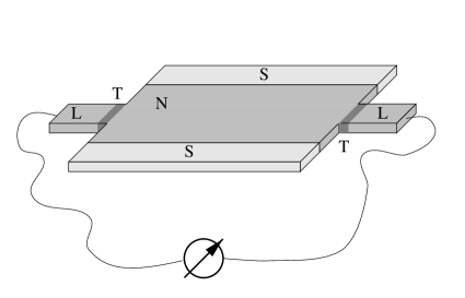
FIG. 1.: Metallic quantum dot (N) in contact with two superconducting regions (S). The dot is separated from the leads (L) by a tunnel barrier (T).

The characteristic feature that distinguishes the above kind of quantum dot from more conventional mesoscopic systems, is the possibility for two electrons to tunnel through the potential barrier at the NS-interface, thereby adding a Cooper pair to (or removing it from) the superconducting condensate. An equivalent statement in single-particle language is that an electron incident on the NS-interface may be retroreflected as a hole (and vice versa). This process of particle-hole conversion, which conserves energy, momentum and spin but violates charge, is called Andreev reflection. In the semiclassical limit, Andreev reflections give rise to numerous almost-periodic orbits whose action does not grow but remains of order $\hbar$ as the length of the orbit increases[9]. The existence of these orbits modifies the mean density of states (Weyl term) of the quantum dot without leads: in general, an excitation gap opens and we arrive at the “boring” situation where the vicinity of the chemical potential is devoid of single-particle states. However, by tuning the phase difference of the order parameters of the two superconducting regions to the special value $\pi$, we can make the gap close. More generally, we expect quasiparticle excitations to exist right at the chemical potential whenever the phase shift incurred during Andreev reflection vanishes on average over the NS-interfacial region. Disorder or dynamically generated chaos mixes the states and creates a universal spectral region close to the chemical potential. Its width is determined by the energy uncertainty which is caused by the coupling of particles and holes by Andreev reflection. It is this very region and its consequences for the transport properties that we are going to study in the present paper.

The organization of the paper is as follows. Mesoscopic independent-quasiparticle systems are classified according to their behavior under time reversal and spin rotations in Sec. II. Having specified the required dynamical input in Sec. III we formulate the appropriate random-matrix ensembles in Sec. IV. In Sec. V we discuss the spectral statistics of an isolated system, using first the Dyson-Mehta orthogonal polynomial method and then diagrammatic perturbation theory. The latter method easily extends to the calculation of the transport properties of an open system. In Sec. VII we work out the weak localization correction to the average conductance and in Sec. VIII the universal conductance fluctuations. Our conclusions are presented in Sec. IX.

II Symmetry Classification

The treatment of this paper is based on the BCS Hamiltonian in the Hartree-Fock-Boboliubov mean-field approximation:

$$\hat{H} = \int d^{d}x\left(\sum_{\sigma,\tau=\uparrow,\downarrow}\psi_{\sigma}^{\dagger}h_{\sigma\tau}\psi_{\tau}+\Delta\psi_{\uparrow}^{\dagger}\psi_{\downarrow}^{\dagger}+\Delta^{*}\psi_{\downarrow}\psi_{\uparrow}\right),$$ (1)

$$h = ({\bf p}-e{\bf A})^{2}/2m+V+{\bf U}_{\rm SO}\cdot\mbox{\boldmath$\sigma$}\times({\bf p}-e{\bf A})-\mu.$$ (2)

Here $V(x)$ is a scalar potential which may have a random component, and $\Delta(x)$ is the pairing field. The presence of a magnetic vector potential ${\bf A}(x)$ breaks time reversal symmetry while the spin-orbit field ${\bf U}_{\rm SO}(x)$ breaks invariance under rotations of the electron’s spin. $\mu$ is the chemical potential.

The second-quantized Hamiltonian $\hat{H}$ can be rewritten in an equivalent first-quantized form by the Boboliubov-deGennes (BdG) formalism. For our purposes it is convenient to introduce some generic orthonormal basis of single-electron states $|\alpha\rangle$, where $\alpha$ is a multi-index that combines the orbital and spin quantum numbers of the electron. If $N$ is the number of orbital states used, $\alpha$ runs from $1$ to $2N$. Let $c_{\alpha}^{\dagger}$ and $c_{\beta}$ be the usual creation and annihilation operators obeying the canonical anticommutation relations $c_{\alpha}^{\dagger}c_{\beta}^{\vphantom{\dagger}}+c_{\beta}^{\vphantom{\dagger}}c_{\alpha}^{\dagger}=\delta_{\alpha\beta}$. The Hamiltonian $\hat{H}$ can be written

$\displaystyle\hat{H}=\sum_{\alpha\beta}\left(h_{\alpha\beta}c_{\alpha}^{\dagger}c_{\beta}^{\vphantom{\dagger}}+{\textstyle{1\over 2}}\Delta_{\alpha\beta}c_{\alpha}^{\dagger}c_{\beta}^{\dagger}+{\textstyle{1\over 2}}\Delta_{\alpha\beta}^{*}c_{\beta}c_{\alpha}\right).$

Hermiticity requires $h_{\alpha\beta}=h_{\beta\alpha}^{*}$, and the matrix elements $\Delta_{\alpha\beta}$ must be antisymmetric by Fermi statistics: $\Delta_{\alpha\beta}=-\Delta_{\beta\alpha}$. Now we write $\hat{H}$ in the form “row multiplies matrix multiplies column”:

$$\hat{H}={1\over 2}\left({\bf c}^{\dagger}\quad{\bf c}\right)\pmatrix{h&\Delta\cr-\Delta^{*}&-h^{\rm T}\cr}\pmatrix{{\bf c}\cr{\bf c}^{\dagger}\cr}+{\rm const}.$$ (3)

In this way every Hamiltonian $\hat{H}$ is uniquely assigned to a $4N\times 4N$-matrix ${\cal H}$,

$${\cal H}=\pmatrix{h&\Delta\cr-\Delta^{*}&-h^{\rm T}\cr}.$$ (4)

The eigenvalue problem for ${\cal H}$ is known as the Bogoliubov-deGennes equations. We refer to ${\cal H}$ as the “BdG-Hamiltonian” for short.

The first-quantized Hamiltonian ${\cal H}$ acts in an enlarged space, namely the tensor product of the physical space ${\bf C}^{2N}$ (orbitals and spin) with an extra degree of freedom ${\bf C}^{2}$, which we call the “particle-hole space”. Note however that the “particles” and “holes” of the BdG-formalism are not the particle and hole states of a degenerate Fermi gas. Indeed, the matrix $h$ already acts on all of the single-electron states, which have energies either above or below the chemical potential. The BdG-hole states acted upon by $-h^{\rm T}$ are identical (and in this sense redundant, or unphysical) copies of the BdG-particle states acted upon by $h$. They are introduced for the convenience of treating the pairing field within the formalism of first quantization.

The aim of the current section is to classify systems according to their symmetries. Using the BdG-formalism we will show that the presence or absence of time-reversal and/or spin-rotation invariance leads to four distinct symmetry classes. The situation thus is different from the well-known Wigner-Dyson scenario where only three distinct classes exist.

The discussion of Secs. II A-II D uses some basic facts from the theory of Lie algebras and symmetric spaces and is somewhat technical. The casual reader may wish to skip these subsections and proceed directly to Table 1 given at the end of Sec. II D. A brief summary of the symmetries of ${\cal H}$ for each class is provided also at the beginning of Sec. IV.

A Symmetry Class $D$

We start by considering systems with the least degree of symmetry, i.e. systems with neither time-reversal symmetry nor spin-rotation invariance. In this case the matrices $h$ and $\Delta$ in general have no symmetry properties beyond those stated above, namely hermiticity of $h$ and skew-symmetry of $\Delta$. Because the set of hermitian matrices does not close under commutation whereas the antihermitian ones do, we prefer to work with $X:=i{\cal H}$ rather than ${\cal H}$ in the current section. In terms of $X$, the conditions $h=h^{\dagger}$, $\Delta=-\Delta^{\rm T}$ can be presented summarily in the form

$$-X^{\dagger} = X=-\Sigma_{x}X^{\rm T}\Sigma_{x},$$ (5)

$$\Sigma_{x} = \pmatrix{0&{\bf 1}_{2N}\cr{\bf 1}_{2N}&0\cr}=\sigma_{x}\otimes{\bf 1}_{2N}.$$ (6)

If two matrices $X,Y$ satisfy these equations, then so does their commutator $[X,Y]$. Hence, we may view $X$ as an element of some Lie algebra. To identify this Lie algebra we conjugate by $X\mapsto\tilde{X}=U_{0}XU_{0}^{-1}$ where $U_{0}={\textstyle{1\over\sqrt{2}}}\left(\begin{array}[]{cc}1&1\\ i&i\end{array}\right)\otimes{\bf 1}_{2N}$. Equations (5) then take the form $-\tilde{X}^{\dagger}=\tilde{X}=-\tilde{X}^{\rm T}$ or, equivalently, $\tilde{X}=\tilde{X}^{*}=-\tilde{X}^{\rm T}$. This shows that (5) fixes a ${\rm so}(4N)$-algebra, i.e. a Lie algebra isomorphic to the real antisymmetric $4N\times 4N$-matrices. Since ${\rm so}(4N)\equiv D_{2N}$ in Cartan’s notation, we denote the present symmetry class by the symbol “$D$”.

Being a Lie algebra element, $X$ can be brought into diagonal form by $X\mapsto\Omega=gXg^{-1}$ where $g$ is an element of the corresponding Lie group which is isomorphic to ${\rm SO}(4N)$ and is defined by

$${g^{-1}}^{\dagger}=g=\Sigma_{x}{g^{-1}}^{\rm T}\Sigma_{x}.$$ (7)

The conditions (5) imply $\Omega={\rm diag}\;\left(i\omega,-i\omega\right)=\sigma_{z}\otimes i\omega$ where $\omega={\rm diag}(\omega_{1},\omega_{2},...,\omega_{2N})$ with real $\omega_{i}$. The conditions for the canonical anticommutation relations to be invariant under a transformation

$\displaystyle\pmatrix{{\bf c}^{\vphantom{\dagger}}\cr{\bf c}^{\dagger}\cr}\mapsto g\pmatrix{{\bf c}^{\vphantom{\dagger}}\cr{\bf c}^{\dagger}\cr}=:\pmatrix{\mbox{\boldmath$\gamma$}^{\vphantom{\dagger}}\cr\mbox{\boldmath$\gamma$}^{\dagger}\cr}$

can be shown[10] to coincide with (7). Thus, inserting $X=g^{-1}\Omega g$ into (3) we obtain

$\displaystyle\hat{H}={1\over 2}\sum_{\lambda}\omega_{\lambda}\left(\gamma_{\lambda}^{\dagger}\gamma_{\lambda}^{\vphantom{\dagger}}-\gamma_{\lambda}^{\vphantom{\dagger}}\gamma_{\lambda}^{\dagger}\right)$

with $\gamma_{\alpha}^{\dagger}\gamma_{\beta}^{\vphantom{\dagger}}+\gamma_{\beta}^{\vphantom{\dagger}}\gamma_{\alpha}^{\dagger}=\delta_{\alpha\beta}$. The frequencies $\omega_{\lambda}$ may be positive or negative. The BCS ground state is defined by demanding $\gamma_{\lambda}|{\rm BCS}\rangle=0$ for $\omega_{\lambda}>0$ and $\gamma_{\lambda}^{\dagger}|{\rm BCS}\rangle=0$ for $\omega_{\lambda}<0$. The normal-ordered Hamiltonian

$\displaystyle:\hat{H}:\ =\sum_{\omega_{\lambda}>0}|\omega_{\lambda}|\gamma_{\lambda}^{\dagger}\gamma_{\lambda}^{\vphantom{\dagger}}+\sum_{\omega_{\lambda}<0}|\omega_{\lambda}|\gamma_{\lambda}^{\vphantom{\dagger}}\gamma_{\lambda}^{\dagger}$

is always positive.

B Symmetry Class $C$

We now consider systems without time-reversal symmetry but with spin-rotation invariance. We again use the unique representation of a second-quantized BCS mean-field Hamiltonian $\hat{H}$ by ($i$ times) a BdG-Hamiltonian $X=i{\cal H}$.

We write the particle-hole decomposition of $X$ as $X=\left(\begin{array}[]{cc}A&B\\ C&D\end{array}\right)$ or, in tensor-product notation,

$\displaystyle X=E_{\rm pp}\otimes A+E_{\rm ph}\otimes B+E_{\rm hp}\otimes C+E_{\rm hh}\otimes D.$

The condition $X=-\Sigma_{x}X^{\rm T}\Sigma_{x}$ means $B=-B^{\rm T}$, $C=-C^{\rm T}$ and $D=-A^{\rm T}$. Antihermiticity requires $A=-A^{\dagger}$ and $C=-B^{\dagger}$.

The generators of spin rotations, $J_{k}$ $(k=x,y,z)$, are represented on particle-hole space by $J_{k}=(E_{\rm pp}\otimes\sigma_{k}-E_{\rm hh}\otimes\sigma_{k}^{\rm T})\otimes{\bf 1}_{N}$. Spin-rotation invariance of the Hamiltonian requires that $X$ and $J_{k}$ commute. This condition is easily seen to constrain $A,B,C$ to be of the form $A={\bf 1}_{2}\otimes a$, $B=i\sigma_{y}\otimes b$ and $C=-i\sigma_{y}\otimes c$ or, in matrix presentation,

$\displaystyle X=\pmatrix{a&0&0&b\cr 0&a&-b&0\cr 0&-c&-a^{\rm T}&0\cr c&0&0&-a^{\rm T}\cr}.$

We see that $X$ decomposes into two commuting subblocks. One corresponds to spin-up particles and spin-down holes, and the other to spin-down particles and spin-up holes. Because the subblocks are related by an algebra homomorphism ($b\mapsto-b$, $c\mapsto-c$) it is sufficient to focus on one of them, say

$\displaystyle X_{\uparrow}=\pmatrix{a&b\cr c&-a^{\rm T}\cr}$

and account for spin degeneracy by inserting factors of two whenever needed. We drop the subscript and write $X$ for $X_{\uparrow}$.

Since $B=-B^{\rm T}$, the equation $B=i\sigma_{y}\otimes b$ implies $b=+b^{\rm T}$. Similarly, we deduce $c=+c^{\rm T}$. Antihermiticity requires $a=-a^{\dagger}$ and $c=-b^{\dagger}$. All these conditions are summarized by

$$-X^{\dagger}=X=-\Sigma_{y}X^{\rm T}\Sigma_{y},\quad\Sigma_{y}=\sigma_{y}\otimes{\bf 1}_{N}.$$ (8)

This is the defining equation of the symplectic Lie algebra ${\rm sp}(2N)$. Thus $X=i{\cal H}$ is an element of ${\rm sp}(2N)$. Since ${\rm sp}(2N)\equiv C_{N}$ in Cartan’s notation, we denote the present symmetry class by “$C$”.

The second-quantized Hamiltonian associated with $X=X_{\uparrow}=\left(\begin{array}[]{cc}a&b\\ c&-a^{\rm T}\end{array}\right)$ is

$\displaystyle\hat{H}_{\uparrow}=-{i\over 2}\sum_{m,n}(c_{m\uparrow}^{\dagger}\quad c_{m\downarrow})\pmatrix{a_{mn}&b_{mn}\cr c_{mn}&-a_{nm}\cr}\pmatrix{c_{n\uparrow}\cr c_{n\downarrow}^{\dagger}}.$

As before, we can diagonalize $X$ by $X=g^{-1}\Omega g$ where $\Omega=\sigma_{z}\otimes i\omega$ and $\omega={\rm diag}(\omega_{1},...,\omega_{M})$, and $g$ now satisfies ${g^{-1}}^{\dagger}=g=\Sigma_{y}{g^{-1}}^{\rm T}\Sigma_{y}$, i.e. $g\in{\rm Sp}(2N)$. The transformation

$\displaystyle\pmatrix{{\bf c}_{\uparrow}\cr{\bf c}_{\downarrow}^{\dagger}\cr}\mapsto g\pmatrix{{\bf c}_{\uparrow}\cr{\bf c}_{\downarrow}^{\dagger}\cr}=:\pmatrix{\mbox{\boldmath$\gamma$}_{\uparrow}\cr\mbox{\boldmath$\gamma$}_{\downarrow}^{\dagger}\cr}$

diagonalizes the Hamiltonian:

$$\hat{H} = \hat{H}_{\uparrow}+\hat{H}_{\downarrow}$$ (9)

$$= {1\over 2}\sum_{\lambda}\omega_{\lambda}\left(\gamma_{\lambda\uparrow}^{\dagger}\gamma_{\lambda\uparrow}^{\vphantom{\dagger}}+\gamma_{\lambda\downarrow}^{\dagger}\gamma_{\lambda\downarrow}^{\vphantom{\dagger}}-\gamma_{\lambda\uparrow}^{\vphantom{\dagger}}\gamma_{\lambda\uparrow}^{\dagger}-\gamma_{\lambda\downarrow}^{\vphantom{\dagger}}\gamma_{\lambda\downarrow}^{\dagger}\right).$$ (10)

Because $g\in{\rm Sp}(2N)\subset{\rm U}(2N)$ is a unitary matrix, the canonical anticommutation relations are preserved by the transformation from $({\bf c},{\bf c}^{\dagger})$ to $(\mbox{\boldmath$\gamma$},\mbox{\boldmath$\gamma$}^{\dagger})$. Every quasiparticle level has a trivial degeneracy due to spin.

C Symmetry Class $D$III

We next consider systems with time-reversal symmetry but without spin-rotation invariance. Recall that the conditions for symmetry class $D$, $-X^{\dagger}=X=-\Sigma_{x}X^{\rm T}\Sigma_{x}$ with $\Sigma_{x}=\sigma_{x}\otimes{\bf 1}_{2}\otimes{\bf 1}_{N}$, fix a ${\rm so}(4N)$-algebra. The time-reversal operator ${\cal T}$ acts on the BdG-Hamiltonian by

$\displaystyle{\cal T}:{\cal H}\mapsto\tau{\cal H}^{*}\tau^{-1}$

where $\tau={\bf 1}_{2}\otimes i\sigma_{y}\otimes{\bf 1}_{N}$. Using $X=i{\cal H}$ and $X^{*}=-X^{\rm T}$ we get the action of ${\cal T}$ on $X$, ${\cal T}:X\mapsto\tau X^{\rm T}\tau^{-1}$. Thus, for a time-reversal invariant system, $X$ is subject to the additional constraint $X=+\tau X^{\rm T}\tau^{-1}$. We denote the set of solutions in ${\rm so}(4N)$ of this condition by ${\cal P}$. While ${\cal P}$ does not close under commutation and therefore does not form a subalgebra of ${\rm so}(4N)$, the solution set, ${\cal K}$, of the complementary condition $Y=-\tau Y^{\rm T}\tau^{-1}$ does. Therefore, we may describe ${\cal P}$ as the complement of a subalgebra ${\cal K}$ in ${\rm so}(4N)$. In formulas, ${\rm so}(4N)={\cal K}+{\cal P}$. We are now going to identify ${\cal K}$.

The equations for ${\cal K}$ can be rewritten

$\displaystyle-Y^{\dagger}=Y=-\Sigma_{x}Y^{\rm T}\Sigma_{x}=-(\Sigma_{x}\tau)Y(\Sigma_{x}\tau)^{-1}.$

Let $U_{0}$ be the unitary matrix given in particle-hole and spin decomposition by

$\displaystyle U_{0}={1\over\sqrt{2}}\pmatrix{{\bf 1}_{2}&i\sigma_{y}\cr\sigma_{y}&-i{\bf 1}_{2}\cr}\otimes{\bf 1}_{N}.$

Conjugation by $U_{0}$, $Y\mapsto\tilde{Y}=U_{0}^{-1}YU_{0}$, takes the equations for ${\cal K}$ into

$\displaystyle-{\tilde{Y}}^{\dagger}=\tilde{Y}=-\Sigma_{x}{\tilde{Y}}^{\rm T}\Sigma_{x}=-\Sigma_{z}{\tilde{Y}}\Sigma_{z}.$

The solutions of the latter are of the form $\tilde{Y}={\rm diag}\;\left(Z,-Z^{\rm T}\right)$ with $Z$ an antihermitian $2N\times 2N$-matrix. We now recognize ${\cal K}$ as being isomorphic to the Lie algebra of antihermitian $2N\times 2N$-matrices, or ${\cal K}\simeq{\rm u}(2N)$. Thus, the space ${\cal P}$ of BdG-Hamiltonians $X=i{\cal H}$ is obtained from ${\rm so}(4N)$ by removing a ${\rm u}(2N)$-subalgebra. Because ${\cal P}$ is the difference of two Lie algebras ${\rm so}(4N)$ and ${\rm u}(2N)$, it can be interpreted as the tangent space of the quotient ${\rm SO}(4N)/{\rm U}(2N)$ of the corresponding Lie groups, which is a symmetric space of type $D$III in Cartan’s notation; hence the name $D$III for the present symmetry class.

From the general theory of symmetric spaces[11] we know that an element $X\in{\cal P}$ can be diagonalized by a transformation $X\mapsto k^{-1}Xk$ with $k\in\exp{\cal K}={\rm U}(2N)$. Time-reversal symmetry causes every eigenvalue to be doubly degenerate by Kramers’ theorem.

D Symmetry Class $C$I

Finally, we turn to systems with both time-reversal symmetry and spin-rotation invariance. Recall that spin-rotation invariance causes the BdG-Hamiltonian $X=i{\cal H}_{\uparrow}$ to obey the relations $-X^{\dagger}=X=-\Sigma_{y}X^{\rm T}\Sigma_{y}$, which define the symplectic Lie algebra ${\rm sp}(2N)$. Because of the restriction to a single spin sector, the action of the time reversal operator simplifies to ${\cal T}:X\mapsto X^{\rm T}$. Thus, time-reversal symmetry constrains $X$ to be symmetric. Let ${\cal K}$ now denote the subalgebra of antisymmetric matrices in ${\rm sp}(2N)$. Then $X$, being symmetric, lies in the complementary set ${\cal P}$ defined by ${\rm sp}(2N)={\cal K}+{\cal P}$. We claim that ${\cal K}$ is isomorphic to the unitary Lie algebra ${\rm u}(N)$. To prove this, we observe that the solutions $Y\in{\cal K}$ of $-Y^{\dagger}=Y=-\Sigma_{y}Y^{\rm T}\Sigma_{y}=Y^{\rm T}$ have the form ${\bf 1}_{2}\otimes{\rm Re}A+i\sigma_{y}\otimes{\rm Im}A$ where $A$ is an arbitrary antihermitian $N\times N$-matrix, i.e. $A\in{\rm u}(N)$. The embedding ${\rm u}(N)\mapsto{\rm sp}(2N)$ by $A\mapsto{\bf 1}_{2}\otimes{\rm Re}A+i\sigma_{y}\otimes{\rm Im}A$ is easily seen to be a homomorphism of Lie algebras. Therefore ${\cal K}\simeq{\rm u}(N)$ as claimed. The linear complement ${\cal P}$ of ${\rm u}(N)$ in ${\rm sp}(2N)$ can be regarded as the tangent space of ${\rm Sp}(2N)/{\rm U}(N)$, which is a compact symmetric space of type $C$I according to Cartan’s list.

For the benefit of the casual reader the various symmetry classes and the names by which they are referred to in the present paper, are summarized in Table 1.

Class	time-rev.	spin-rot.	sym. space
$D$	no	no	SO(4$N$)
$C$	no	yes	Sp(2$N$)
$D$III	yes	no	SO(4$N$)/U(2$N$)
$C$I	yes	yes	Sp(2$N$)/U($N$)

Table 1

E Is the symmetry (5) wiped out by Coulomb effects?

The symmetry (5) is central to our approach. Just how robust is it?

The relations (5) follow from the well-known mathematical fact[10] that the set of all bilinear combinations of the fermion creation and annilihation operators is isomorphic to an orthogonal Lie algebra. Put differently, the symmetry (5) requires no more than the fermionic nature of the electron and the use of the Hartree-Fock-Bogoliubov mean-field approximation, allowing us to express the Hamiltonian in terms of bilinears of the creation and annihilation operators. Alternatively, we could say that (5) is an exact symmetry whenever the system can be described in terms of independent Boboliubov quasiparticles.

What happens when we add a Coulomb charging energy to the Hamiltonian? The relative minus sign between the particle-particle and hole-hole blocks of ${\cal H}$, Eq. (4), tells us that, if the creation of an electron in a given state costs a certain amount of energy, then the creation of a hole (removal of an electron) in this state should release exactly the same amount. The Coulomb interaction, however, does not conform to that principle. When a charge is added to a charge-neutral system, say, it makes no difference whether this charge is a particle or a hole, the electrostatic energy cost is positive in both cases. Therefore, the Coulomb charging energy (as well as other perturbations that do not fit into the independent-quasiparticle framework) violates the symmetry (5). More precisely speaking, we expect the independent-quasiparticle approximation to be adequate for describing the short-time physics, but at sufficiently long times Coulomb effects must become visible and, in particular, they will cut off the particle-hole modes we are going to study in the present paper. Whether the cutoff time can be long enough for the consequences of the symmetry (5) to be observable, is a tough quantitative question for theory, which cannot be answered without an understanding of screening in open and finite metallic systems. Fortunately, the question has already been answered in the affirmative by experiment. Over the last years a number of novel mesoscopic NS-phenomena has been observed, the most prominent of which is the dramatic enhancement[12] of the differential conductance at zero bias in NS-geometries with a high potential barrier separating the normal-conducting and superconducting regions. This phenomenon has been explained[13] by a mechanism called “coherent Andreev reflection” or “reflectionless tunneling”[14], which is the result of constructive interference between semiclassical paths with one Andreev reflection and a variable number of normal reflections. In order for such an interference to take place, the dynamical phases of a particle and a hole traversing the same path in opposite directions must cancel each other. It is precisely the symmetry (5) in combination with the extra symmetries defining class $C$I, that guarantee the necessary phase relation between particles and holes to hold. We conclude that there exists convincing experimental evidence that the symmetry (5) is not wiped out by the Coulomb interaction but leads to observable consequences. In the remainder of this paper we are going to ignore Coulomb effects.

III Dynamical Input

The classification of Sec. II refers only to symmetry and thus is very general. To go further, we make two dynamical assumptions.

When an electron is retroreflected from the NS-interface as a hole, its wavefunction acquires a phase shift which is determined by the phase of the superconducting order parameter. Our first assumption is that this phase shift, here called the “Andreev phase shift” for short, vanishes on average over the NS-interfacial region. To appreciate what such an assumption implies, let us look at a few examples. Consider first an SNS-system consisting of an infinite slab of normal metal sandwiched between two superconducting slabs $S_{1}$ and $S_{2}$. The pairing interaction causes the existence of an excitation gap in each of the superconducting regions. We now ask how the presence of the normal-conducting slab affects the excitation spectrum of the combined SNS-system at the chemical potential. The answer to this question was first given in[15, 16] and it is essentially as follows. In the clean limit, the BdG-Hamiltonian is separable and we can get a qualitative understanding of the quantal energy spectrum by the method of semiclassical quantization. For simplicity we assume that all reflections at the NS-interface are Andreev. Every periodic classical motion then is some multiple of a primitive periodic orbit where an electron moves back and forth between the superconducting regions and is Andreev reflected at each interface. If $k_{\rm p}$ ($k_{\rm h}$) are the wave numbers of the particle (hole) normal to the slabs and $L$ is the thickness of the normal-conducting region, the Bohr-Sommerfeld quantization rule applied to this periodic motion reads

$$\pm(k_{\rm p}-k_{\rm h})L+\pi+\varphi_{1}-\varphi_{2}=2\pi n\qquad(n\in{\bf Z}).$$ (11)

Here $\pi+\varphi_{1}-\varphi_{2}$ is the phase accumulated by the two Andreev reflections if $\varphi_{1}$ and $\varphi_{2}$ are the phases of the superconducting order parameter in the regions $S_{1}$ and $S_{2}$. For an electron with energy equal to the Fermi energy, $k_{\rm p}$ equals $k_{\rm h}$, so the first term on the left-hand side vanishes. From the resulting equation $\varphi_{1}-\varphi_{2}=(2n-1)\pi$ we see that the quantization condition can be fulfilled only when $\varphi_{1}$ and $\varphi_{2}$ differ by an odd multiple of $\pi$. In other words, for $\cos(\varphi_{1}-\varphi_{2})\not=-1$, which includes the homogeneous case $\varphi_{1}=\varphi_{2}$, we expect a gap in the excitation spectrum not only in the superconductor but also in the combined SNS-system. On the other hand, for $\cos(\varphi_{1}-\varphi_{2})\to-1$ the gap closes and quasiparticle excitations exist all the way down to zero energy. The latter situation is special in that the Andreev phase shift vanishes on average over the two NS-interfaces in that case.

The above argument applies to the extreme limit of a clean system which clearly is unrealistic. What can we say about the effects of disorder? A generic random potential destroys separability and makes Bohr-Sommerfeld quantization inapplicable. The general case therefore needs to be studied with the help of a computer, or by using the random-matrix theory that will be developed in the remainder of our paper. What is easy to treat analytically is the case of a slowly varying random potential depending only on the coordinate, $z$, of the direction perpendicular to the slabs. In this case the quantization rule (11) remains valid if we replace the expression $(k_{\rm p}-k_{\rm h})L$ by the integral $\int_{0}^{L}\Bigl{(}k_{\rm p}(z)-k_{\rm h}(z)\Bigr{)}dz$ where $k_{\rm p}(z)=[2m(\mu+\varepsilon-V(z)]^{1/2}$, $k_{\rm h}(z)=[2m(\mu-\varepsilon-V(z)]^{1/2}$, and $E=\mu+\varepsilon$ is the total energy of the electron. Since $k_{\rm p}(z)=k_{\rm h}(z)$ for $\varepsilon=0$, our conclusions are the same as before: there is a gap for $\cos(\varphi_{1}-\varphi_{2})\not=-1$, and the gap closes as $\cos(\varphi_{1}-\varphi_{2})\to-1$.

Another instructive example is provided by the vortex solution for a clean type-II superconductor. The phase of the superconducting order parameter uniformly winds once around the unit circle as we go once around the vortex core. For this reason, the pairing field experienced by normal excitations bound to the vortex core vanishes on average over the vortex. Because the vortex solution breaks translational symmetry, there must exist some RPA (or vibrational) zero modes of the vortex. These zero modes are the Goldstone modes associated with the spontaneous breaking of translational symmetry by the localized vortex solution. It follows that, if the RPA correlation energy vanishes (is small), i.e. if the excitation energies are given by (are approximately given by) sums of two quasiparticle energies, there must exist quasiparticle excitations with vanishing (small) energy. In contrast, for a piece of cylindrically shaped normal metal immersed in a superconducting environment (“columnar defect”) there is no general reason why we should expect quasiparticle excitations with low energy.

These two examples, the SNS slab geometry and the vortex, lend support to the plausible expectation that a pairing field which is locally nonzero but whose mean phase $\langle e^{i\phi}\rangle$ vanishes in a suitably defined sense, is ineffective at creating a genuine gap in the density of states near the chemical potential. This then is the motivation behind the above requirement that the Andreev phase shift should vanish on average over the NS-interfacial region: it ensures that the gap closes and quasiparticles can exist right at the chemical potential.

Our second main input is the assumption that the classical dynamics in the normal-conducting (N-) region be chaotic. The presence of a sufficient amount of disorder will always guarantee this assumption to be justified. For a ballistic system, chaotic dynamics is achieved by choosing for the boundary of the N-region some surface that causes a typical classical trajectory to be unstable. Chaoticity of the classical motion means that the long-time behavior of the system is unpredictable; in particular, the phase shifts acquired by Andreev reflection along a typical semiclassical trajectory form a random sequence. This randomness will allow us to model the pairing field by a stochastic variable. Note that the spatial constancy of the magnitude of the pairing field in the bulk of the superconductor is an irrelevant feature for our purposes. If we switch from coordinate representation to a generic basis of single-particle states, say the eigenbases of $h$ and $-h^{\rm T}$, both the phase and the magnitude of $\Delta$ will fluctuate and be distributed around zero.

Consider now an isolated finite system, so that the Boboliubov quasiparticle spectrum is discrete. According to our above arguments, we expect the existence of levels close to the chemical potential in the pure system under the conditions described. The effect of dynamically generated chaos and/or disorder will be to cause mixing of these levels. For the conventional N-system, such mixing is known to lead to universal level statistics, depending only on symmetry. (More precisely, the level correlations are universal in the low-frequency regime corresponding to the long-time or ergodic limit.) For the case of disordered metallic granules, the level correlations were calculated by Efetov[3]. His results show that the level statistics is Wigner-Dyson, i.e. identical to that of an ensemble of random matrices with uncorrelated Gaussian distributed matrix elements. In the NS-systems considered in the present paper, new features appear at low excitation energy, owing to the coupling of particles and holes by the process of Andreev reflection at the NS-interface. As was shown in Sec. II, the presence of the pairing field $\Delta$ leads to novel symmetries. We therefore expect new types of universal level statistics to emerge in such systems. The new type of correlation will extend over an energy range set by the energy uncertainty due to the action of the pairing field (or Andreev reflection). The goal of our paper is to give a quantitative description of precisely these correlations and their effect on the transport properties. To reach this goal we may follow two different routes. The first and more comprehensive one is to generalize Efetov’s analysis, i.e. to construct an effective field theory of the nonlinear $\sigma$ model type and solve the field theory in the zero-dimensional limit corresponding to the universal regime. Such an approach yields not only the universal behavior but also the crossover to the short-time regimes. Since our interest is in the universal limit, there exists also another option. Armed by the experience gained from the study of the N-system, we may replace the BdG-Hamiltonian (4) by an ensemble of random matrices with maximum entropy, paying attention only to the symmetries under time reversal and spin rotation. While the field-theoretic method is more versatile, the random-matrix or maximum-entropy approach has the great advantage of being much simpler technically. For this reason we have chosen to follow the latter in the present paper.

To maximize the entropy of the random-matrix ensemble we will take the matrix elements of the BdG-Hamiltonian to be normally distributed and statistically independent. All matrix elements will be chosen to have zero mean. For the off-diagonal blocks of the BdG-Hamiltonian, this choice corresponds to our assumption that the spatial average of the Andreev phase shift vanishes on average. In general, we would need to distinguish between the strength of fluctuation of $h$ and $\Delta$. However, at low energy, i.e. within the energy window defined by the uncertainty due to Andreev reflection, this distinction turns out to be irrelevant and we may take the strengths to be equal. The resulting random-matrix ensemble depends on two parameters only. These are the strengths of the perturbations that break time-reversal and spin-rotation invariance and are responsible for the crossover between universality classes.

To finish off this orientational section, we mention another realm of application of the above random-matrix ideas. Consider an array of superconducting grains or islands embedded in a metallic (non-superconducting) host. The grains are disordered and/or of irregular shape, and they are mutually coupled by Josephson tunnelling. The array is exposed to a subcritical magnetic field which penetrates the host but is ejected from the grains. By tuning the strength of the field we can frustrate the coupling between the grains and drive the system into a spin-glass type of phase where superconducting order exists locally but not globally. Such a system has been called a superconducting glass[6]. Its prime characteristic is that the pairing field, or superconducting order parameter, continues to be nonzero on each grain but vanishes on average over large scales. The low-energy quasiparticle excitations of such a system are predicted to be described by the random-matrix model formulated below. Because of the breaking of time-reversal symmetry by the magnetic field, the relevant symmetry class is $C$. The presence of spin-orbit interactions causes crossover to $D$.

IV Random-Matrix Ensembles

To prepare the formulation of the random-matrix ensembles, we summarize the discussion of Sec. II by presenting the symmetries of the BdG-Hamiltonian ${\cal H}$ for each symmetry class explicitly.

For systems where all symmetries are broken (class $D$) ${\cal H}$ satisfies ${\cal H}=-\Sigma_{x}{\cal H}^{\rm T}\Sigma_{x}$ with $\Sigma_{x}=\sigma_{x}\otimes{\bf 1}_{2}\otimes{\bf 1}_{N}$. The block decomposition

$\displaystyle{\cal H}=\pmatrix{A&B\cr B^{\dagger}&-A^{\rm T}\cr}$

expresses the particle-hole structure of ${\cal H}$. The off-diagonal block $B$ is antisymmetric by Fermi statistics. Hermiticity of the Hamiltonian requires $A=A^{\dagger}$.

Class $D$III consists of the systems where time reversal is the only good symmetry. For such systems ${\cal H}$ obeys the additional relation ${\cal H}=\tau{\cal H}^{\rm T}\tau^{-1}$ with $\tau={\bf 1}_{2}\otimes i\sigma_{y}\otimes{\bf 1}_{N}$. The decomposition of ${\cal H}$ according to particles and holes (outer block structure) and spin (inner block structure) has the form

$\displaystyle{\cal H}=\pmatrix{a_{\uparrow\uparrow}&a_{\uparrow\downarrow}&b_{\uparrow\uparrow}&b_{\uparrow\downarrow}\cr a_{\downarrow\uparrow}&a_{\uparrow\uparrow}^{\rm T}&-b_{\uparrow\downarrow}^{\rm T}&b_{\downarrow\downarrow}\cr-b_{\downarrow\downarrow}&-b_{\uparrow\downarrow}^{\rm T}&-a_{\uparrow\uparrow}^{\rm T}&a_{\downarrow\uparrow}\cr b_{\uparrow\downarrow}&-b_{\uparrow\uparrow}&a_{\uparrow\downarrow}&-a_{\uparrow\uparrow}\cr}$

with antisymmetric $a_{\uparrow\downarrow}$, $a_{\downarrow\uparrow}$, $b_{\uparrow\uparrow}$ and $b_{\downarrow\downarrow}$. Hermiticity of ${\cal H}$ requires $a_{\uparrow\uparrow}=a_{\uparrow\uparrow}^{\dagger}$, $b_{\uparrow\downarrow}=b_{\uparrow\downarrow}^{\dagger}$, $a_{\uparrow\downarrow}=a_{\downarrow\uparrow}^{\dagger}$, and $b_{\downarrow\downarrow}=-b_{\uparrow\uparrow}^{\dagger}$.

For class $C$ spin is conserved while time-reversal symmetry is broken. In this case ${\cal H}$ commutes with the spin-rotation generators $J_{k}=(E_{\rm pp}\otimes\sigma_{k}-E_{\rm hh}\otimes\sigma_{k}^{\rm T})\otimes{\bf 1}_{N}$ or, equivalently, ${\cal H}$ obeys ${\cal H}=J_{k}{\cal H}J_{k}$. The particle-hole and spin decomposition of ${\cal H}$ reads

$\displaystyle{\cal H}=\pmatrix{a&0&0&b\cr 0&a&-b&0\cr 0&-b^{\dagger}&-a^{\rm T}&0\cr b^{\dagger}&0&0&-a^{\rm T}\cr}$

with symmetric $b$. Every level has a trivial twofold degeneracy due to spin. Without loss of information we may focus on the spin-up sector with reduced Hamiltonian

$\displaystyle{\cal H}_{\rm r}=\pmatrix{a&b\cr b^{\dagger}&-a^{\rm T}\cr}.$

Hermiticity requires $a=a^{\dagger}$.

In class $C$I both spin rotations and time reversal are good symmetries. The BdG-Hamiltonian satisfies ${\cal H}=\tau{\cal H}^{\rm T}\tau^{-1}=J_{k}{\cal H}J_{k}$, and is constrained by these symmetries to be of the form

$\displaystyle{\cal H}=\pmatrix{a&0&0&b\cr 0&a&-b&0\cr 0&-b&-a^{\rm T}&0\cr b&0&0&-a^{\rm T}\cr}$

with symmetric $a$ and $b$. Hermiticity then implies that $a$ and $b$ are real matrices.

Now recall the dynamical conditions formulated in Sec. III. By assumption, the classical dynamics in the N-system is chaotic and the Andreev phase shift vanishes on average over the NS-interfacial region. We therefore may replace the BdG-Hamiltonian by a random matrix (of the appropriate symmetry) with matrix elements that have zero mean. The principle of least information, or maximum entropy, then leads us to postulate a random-matrix ensemble with a Gaussian probability distribution

$$\exp\left(-{\rm Tr}{\cal H}^{2}/2v^{2}\right)d{\cal H}$$ (12)

for each symmetry class. Here $d{\cal H}$ denotes a Euclidean measure on the linear space of BdG-Hamiltonians with metric ${\rm Tr}(d{\cal H})^{2}$.

More generally, we can formulate a two-parameter family of Gaussian random-matrix ensembles which interpolates between all four symmetry classes. Because a Gaussian distribution (with zero mean) is completely specified by its second moment, it is sufficient to describe the correlation function $\langle{\rm Tr}{\cal AH}\times{\rm Tr}{\cal BH}\rangle$ for two arbitrary sources ${\cal A}$ and ${\cal B}$. The correlation law we choose is

$$\langle{\rm Tr}{\cal AH}\times{\rm Tr}{\cal BH}\rangle/v^{2}$$ (13)

$$= {\rm Tr}({\cal A}-\Sigma_{x}{\cal A}^{\rm T}\Sigma_{x})\Bigl{[}{\cal B}+(1-\epsilon_{t})\tau{\cal B}^{\rm T}\tau^{-1}$$ (16)

$$\hskip 99.58464pt+(1-\epsilon_{s})\sum_{k}J_{k}{\cal B}J_{k}$$

$$\hskip 42.67912pt+(1-\epsilon_{s})(1-\epsilon_{t})\sum_{k}J_{k}\tau B^{\rm T}\tau^{-1}J_{k}\Bigr{]}.$$

For $\epsilon_{s}=\epsilon_{t}=0$ the correlation law is invariant under both reversal of time and rotation of spin. This is the symmetry class $C$I. A nonzero value of $\epsilon_{t}$ breaks time-reversal symmetry. Therefore, by increasing $\epsilon_{t}$ we cross over to class $C$. A nonzero value of $\epsilon_{s}$ breaks spin-rotation invariance, so by increasing $\epsilon_{s}$ we cross over to class $D$III. By increasing both $\epsilon_{s}$ and $\epsilon_{t}$ we break all symmetries and cross over to class $D$. We call a symmetry “maximally broken” when its symmetry-breaking parameter ($\epsilon_{s}$ or $\epsilon_{t}$) equals unity. Whenever a symmetry is either unbroken or maximally broken, the probability distribution of the Gaussian ensemble can be presented in the simple form (12), with the corresponding symmetry constraints imposed on ${\cal H}$.

All information about the level statistics is contained in the joint probability distribution for the eigenvalues, $P(\{\omega\})$. This distribution is a complicated function in general, but it takes a simple form for each universality class. By diagonalizing the BdG-Hamiltonian

$\displaystyle{\cal H}=U\pmatrix{\omega&0\cr 0&-\omega\cr}U^{-1},\quad\omega={\rm diag}(\omega_{1},\omega_{2},...)$

and computing the Jacobian of the transformation to diagonal form, we obtain the formula

$$P(\{\omega\})d\{\omega\}=\prod_{i<j}|\omega_{i}^{2}-\omega_{j}^{2}|^{\beta}\prod_{k}|\omega_{k}|^{\alpha}e^{-\omega_{k}^{2}/v^{2}}d\omega_{k}$$ (17)

where, for the individual cases,

$${\rm class\ }D:\quad\beta=2,\quad\alpha=0;$$ (18)

$${\rm class\ }C:\quad\beta=2,\quad\alpha=2;$$ (19)

$${\rm class\ }D{\rm III}:\quad\beta=4,\quad\alpha=1;$$ (20)

$${\rm class\ }C{\rm I}:\quad\beta=1,\quad\alpha=1.$$ (21)

These expressions for $P(\{\omega\})$ can be derived by elementary means. A particularly elegant derivation uses the interpretation of ${\cal H}$ as being tangent to the symmetric space of type $D$, $D$III, $C$, or $C$I. The Jacobian can then be read off immediately from the tabulated root systems of these spaces.

The formula for $P(\{\omega\})$ permits some immediate conclusions to be drawn. Clearly, the significance of the parameter $\alpha$ is that it governs the level repulsion from the origin $\omega=0$, while $\beta$ gives the mutual repulsion between levels. For the following it is useful to view the factor $|\omega_{k}|^{\alpha}$ as being due to the interaction of the $k^{\rm th}$ level with its “image” at $-\omega_{k}$. Similarly we view the factor $\omega_{i}+\omega_{j}$ in $\omega_{i}^{2}-\omega_{j}^{2}$ as resulting from the interaction of the $i^{\rm th}$ level with the image of the $j^{\rm th}$ level. At energies $\omega$ much greater than the mean level spacing, the interaction of levels with their distant images at negative energies is expected to be irrelevant. Therefore the level statistics derived from (17) will reduce, in that limit, to the usual Wigner-Dyson statistics as determined by the parameter $\beta$. On the other hand, in the opposite limit of energies of order unity on the scale set by the level spacing, the level statistics will be different from Wigner-Dyson. In particular, by the definition of $P(\{\omega\})$ as a joint probability density we immediately conclude that the mean density of levels near zero behaves as

$$\langle\rho(\omega)\rangle=\langle{\rm Tr}\delta(\omega-{\cal H})\rangle\sim|\omega|^{\alpha}\quad(\omega\to 0).$$ (22)

Note that for the systems where our random-matrix description applies, the exponent $\alpha$ is predicted to be universal, dependent only on symmetry. The value of $\alpha$ for the symmetry classes $C$I and $C$ is easily understood from the fact that the repulsion of a level from its own image is caused by the pairing field $\Delta$. For class $C$ pairing matrix elements are complex, whereas for class $C$I all pairing matrix elements can be chosen to be real. By a standard power counting argument this results in $\alpha=2$ and $\alpha=1$ respectively. To understand why $\alpha$ is zero for class $D$, note that in this case a level and its own image are not really physically distinct but are copies of the same single-electron state. (In contrast, for the classes $C$ and $C$I the hole level has its spin flipped relative to the particle level.) The pairing matrix element between identical states vanishes by the Pauli principle – or put differently, the matrix $\Delta$ in (4) is antisymmetric and therefore has zeroes on its diagonal –, which results in $\alpha=0$.

V Spectral Statistics

A Exact Results

Our interest here is in the level correlations for a large matrix dimension $2N$. These are easy to compute when the symmetry class is $C$ or $D$. Consider first class $C$. For this symmetry class we can interpret $P(\{\omega\})$ as the joint probability density of a Gaussian Unitary Ensemble (GUE) of $2N$ levels $\omega_{1},\omega_{\bar{1}},...,\omega_{N},\omega_{\bar{N}}$ subject to the mirror constraint $\omega_{\bar{k}}=-\omega_{k}$. The GUE joint probability density, in turn, can be interpreted as the square of the ground state wavefunction for a system of spinless nonrelativistic noninteracting 1D fermions confined by a harmonic well[17]. This correspondence of levels and Fermi particles turns the $n$-level correlation functions of the GUE into the $n$-point static density correlation functions of the Fermi system. In the large-$N$ limit, the spatial variation of the harmonic confining potential becomes (locally) negligible and the gas of fermions can be treated as locally free. The mirror constraint means that whenever a fermion approaches zero, then so does its mirror image. Because the Pauli principle makes the wavefunction vanish as two fermions approach each other, this amounts to hard wall (or Dirichlet) boundary conditions at $\omega=0$. Hence we can compute the level density and its correlations as the particle density and its correlations for a free 1D Fermi gas with Dirichlet boundary conditions at the origin. The free-fermion wavefunctions that vanish at $\omega=0$ are $\sin(\omega\tau)$, where $\tau$ plays the role of a “wavenumber”. By summing over the Fermi sea of states occupied in the ground state, we obtain for the mean density of levels

$$\langle\rho(\omega)\rangle={2\over\pi}\int_{0}^{\pi}\sin^{2}(\omega\tau)d\tau=1-{\sin 2\pi\omega\over 2\pi\omega}.$$ (23)

Here and throughout this subsection we follow the convention of measuring $\omega$ in units of the mean spacing between neighboring particles (i.e. of the level spacing) at a distance of many spacings from zero. Note that $\langle\rho(\omega)\rangle$ for $\omega\to 0$ has the behavior expected from (22) (recall $\alpha=2$ for class $C$). A similar calculation of the density-density correlator of the Fermi gas yields the two-level cluster function:

$$\langle\rho(\omega_{1})\rho(\omega_{2})\rangle-\langle\rho(\omega_{1})\rangle\langle\rho(\omega_{2})\rangle$$ (25)

$$-\big{[}\delta(\omega_{1}-\omega_{2})+\delta(\omega_{1}+\omega_{2})\big{]}\langle\rho(\omega_{1})\rangle$$

$$= -\left[{\sin\pi(\omega_{1}-\omega_{2})\over\pi(\omega_{1}-\omega_{2})}-{\sin\pi(\omega_{1}+\omega_{2})\over\pi(\omega_{1}+\omega_{2})}\right]^{2}.$$ (26)

Keeping $r=\omega_{1}-\omega_{2}\not=0$ fixed and letting $\omega_{1}+\omega_{2}$ tend to infinity, we recover the familiar GUE two-level cluster function $-\sin^{2}(\pi r)/(\pi r)^{2}$. Similarly, all $n$-level functions $R_{n}(\omega_{1},...,\omega_{n})=\langle\rho(\omega_{1})...\rho(\omega_{n})\rangle$ can be calculated. On subtracting the level self-correlations, which amounts to normal ordering in the particle-gas formulation, we obtain the result

$$R_{n}(\omega_{1},...,\omega_{n}) = {\rm Det}\left[\Psi_{C}(\omega_{i},\omega_{j})\right]_{i,j=1,...,n}\ ,$$ (27)

$$\Psi_{C}(\omega_{i},\omega_{j}) = {2\over\pi}\int_{0}^{\pi}\sin(\omega_{i}\tau)\sin(\omega_{j}\tau)d\tau,$$ (28)

by simply using Wick’s theorem for the free Fermi gas.

We turn to the symmetry class $D$. It is convenient again to use the interpretation of the joint probability density as a Gaussian Unitary Ensemble of $2N$ levels with a mirror constraint. The only change from before is that the repulsion of a level from its own mirror image is now absent ($\alpha=0$). Correspondingly the single-fermion wavefunctions of the Fermi gas no longer vanish on approaching the origin. Instead, what we need to demand is that they be even functions of $\omega$, which is the same as imposing vanishing derivative (or Neumann) boundary conditions at $\omega=0$. Thus the level $\leftrightarrow$ particle correspondence now leads to the free Fermi gas with Neumann boundary conditions at the origin. Doing the same kind of calculation as before we find

$$\langle\rho(\omega)\rangle={2\over\pi}\int_{0}^{\pi}\cos^{2}(\omega\tau)d\tau=1+{\sin(2\pi\omega)\over 2\pi\omega},$$ (29)

and the result (27) remains valid if we replace $\Psi_{C}$ by $\Psi_{D}$,

$\displaystyle\Psi_{D}(\omega_{i},\omega_{j})={2\over\pi}\int_{0}^{\pi}\cos(\omega_{i}\tau)\cos(\omega_{j}\tau)d\tau.$

From (29) we see that for a metallic quantum dot with spin-orbit scattering (class $D$), the proximity of a superconductor with $\langle e^{i\phi}\rangle=0$ enhances the level density at the chemical potential! While this effect may seem physically surprising, it is very natural in the Fermi-gas picture of the levels. The pressure of the gas pushes particles (or levels) against the “wall” at $\omega=0$. Because it is the current rather than the density that is required to vanish by the Neumann boundary condition, an excess particle density forms at the wall such that the extra statistical force balances the pressure.

More effort is required by the symmetry classes $C$I and $D$III, where $\beta=1$ and $\beta=4$. It is still possible in these cases to map the level statistics problem on a model of particles moving on a half line, but progress is slowed down by the fact that the particles now interact with each other. By a standard transformation[18] one can show that their motion is governed by the Hamiltonian of the Calogero-Sutherland model (CSM) associated with the symmetric spaces of type $C$I and $D$III. For the case of the CSMs corresponding to the Wigner-Dyson Ensembles, it was recently found[19] that the CSM particles behave as a gas of free anyons, i.e. particles with fractional charge and statistics. Although we have some preliminary results indicating that the free anyon gas picture can be adapted to the present situation, the details have not been worked out yet.

A quick way to get the infrared (or large-$\omega$) asymptotics of the level density for $C$I and $D$III is to bosonize[20] the CSM. This procedure has been argued[21] to yield the $c=1$ conformal field theory of a free boson with compactification radius $R=\sqrt{\beta/2}$. The expression for the CSM particle density $\bar{\psi}\psi$ in terms of the boson field $\varphi$ is[22]

$$\bar{\psi}\psi=\partial_{\omega}\varphi+{\rm const}\times\cos(\sqrt{4\pi}\varphi/R+k_{F}\omega).$$ (30)

(Recall that by the level $\leftrightarrow$ particle correspondence $\omega$ is to be interpreted as a space coordinate here.) The mirror constraint of the CSM for $C$I and $D$III translates into a boundary condition on $\varphi$ at $\omega=0$. Since the vertex operator $\exp(\sqrt{4\pi}i\varphi/R)$ has the scaling dimension $1/R^{2}=2/\beta$, we expect

$$\langle\rho(\omega)\rangle=1+\omega^{-2/\beta}A_{\beta}(\omega)+...$$ (31)

where $A_{\beta}(\omega)$ is a function that oscillates with a period determined by the mean spacing. Note that (31) is consistent with the $\beta=2$ results (23) and (29). Note also that the first term on the right-hand side of (30) gives a vanishing contribution to the average density, although it does contribute to the CSM density-density correlator. This is because the current $\partial_{\omega}\varphi$, being linear in the boson field $\varphi$, has a vanishing expectation value even when there is a boundary.

The validity of bosonization and conformal field theory arguments is restricted to the infrared regime. To obtain expressions that are valid in the entire range of frequencies $\omega$, we turn to the orthogonal polynomial method of Dyson and Mehta[23]. The substitution $x_{k}=\omega_{k}^{2}$ turns (17) for $\alpha=1$ into

$\displaystyle p(\{x\})d\{x\}={\rm const}\times\prod_{i<j}|x_{i}-x_{j}|^{\beta}\prod_{k}e^{-x_{k}/v^{2}}dx_{k},$

which defines what has been called[24] the Laguerre Orthogonal Ensemble (LOE) for $\beta=1$, and the Laguerre Symplectic Ensemble (LSE) for $\beta=4$. Note that this nomenclature is rather unfortunate in the present context. As we saw, the LOE relates to the symmetric space ${\rm Sp}(2N)/{\rm U}(N)$, while the LSE relates to the symmetric space ${\rm SO}(4N)/{\rm U}(2N)$. In both cases the invariance group is a unitary group, ${\rm U}(N)$ or ${\rm U}(2N)$. Closed expressions for the $n$-level correlation functions of these ensembles have recently been published by Nagao and Slevin[24]. By using some identities for Bessel functions and returning to the variable $\omega=x^{2}$, we can cast their results for the mean density in the form

$$C{\rm I}:\quad\langle\rho(\omega)\rangle = F(\pi\omega),$$ (32)

$$D{\rm III}:\quad\langle\rho(\omega)\rangle = F(2\pi\omega)+\pi J_{1}(2\pi\omega)/2,$$ (33)

$$F(z) = {\pi\over 2}\int_{0}^{z}dt\ J_{0}(t)J_{1}(t)/t,$$ (34)

where $J_{k}$ is the Bessel function of order $k$. (Remember that we are taking the level spacing at large $\omega$ for our energy unit. The levels are counted without multiplicity.) From this we read off the small-$\omega$ expansions:

$\displaystyle\langle\rho(\omega)\rangle=\beta\pi^{2}\omega/4+{\cal O}(\omega^{3})\qquad(C{\rm I}\ {\rm and}\ D{\rm III}).$

Knowing the mean density, we can construct the full one-point function $\langle g(\omega)\rangle=\langle{\rm Tr}(\omega+i\delta-{\cal H})^{-1}\rangle$ by causality, i.e. by using the dispersion relation that connects the real and imaginary parts of a holomorphic function on the upper complex half-plane. The results can be presented in the form

$$C{\rm I}:\quad \langle g(\omega)\rangle$$ (35)

$$= -i\pi+i\int_{1}^{\infty}du\int_{-1}^{+1}dv\ {\sqrt{1-v^{2}}\over\sqrt{u^{2}-1}}{e^{i\pi\omega(u-v)}\over u-v},$$ (36)

$$D{\rm III}:\quad \langle g(\omega)\rangle=-i\pi+i\pi\int_{1}^{\infty}du\ {u\over\sqrt{u^{2}-1}}e^{2i\pi\omega u}$$ (38)

$$-i\int_{1}^{\infty}du\int_{-1}^{+1}dv\ {\sqrt{u^{2}-1}\over\sqrt{1-v^{2}}}{e^{2i\pi\omega(u-v)}\over u-v}.$$

Although it is hard work to construct these expressions directly, they can easily be verified. For that we simply differentiate the result for $\langle g(\omega)\rangle$ with respect to $\omega$, thereby cancelling the factor $u-v$ in the denominator of the double integrals. The integrals over $u$ and $v$ then separate, and on taking the imaginary part each integral produces a Bessel function. By using standard recursion relations for these functions and then undoing the $\omega$-differentiation by integration, we immediately retrieve the expressions for $\langle\rho(\omega)\rangle$ given earlier.

The double integrals for $C$I ($\beta=1$) and $D$III ($\beta=4$) are seen to be related by a duality transformation that exchanges the compact ($v$) and noncompact ($u$) degrees of freedom. A similar duality relation holds for the conventional Wigner-Dyson ensembles with $\beta=1$ and $\beta=4$[3]. In the limit of large $\omega$ we get the following asymptotic expansions for the one-point function:

$$C{\rm I}:\quad\langle g(\omega)\rangle = -i\pi-{1\over 2\omega}+{1\over 4\pi\omega^{2}}e^{2\pi i\omega}+...$$ (39)

$$D{\rm III}:\quad\langle g(\omega)\rangle = -i\pi+{1\over 4\omega}+{i\pi\over 2\sqrt{\omega}}e^{2\pi i\omega+i\pi/4}+...$$ (40)

For completeness, the one-point functions for the symmetry classes $C$ and $D$ ($\beta=2$), as determined from (23) and (29) by causality, are

$\displaystyle\langle g(\omega)\rangle=-i\pi+(1-\alpha){1-e^{2\pi i\omega}\over 2\omega}\quad(C\ {\rm and}\ D).$

By comparing with (31) we see that the oscillatory correction to the stationary asymptotic limit $\langle g(\omega)\rangle\to-i\pi$ agrees with what is expected from the conformal limit of the Calogero-Sutherland model, in all cases. The smooth ($1/\omega$) part of the correction is purely real and does not enter into the asymptotic expression for the density of states.

The authors of Ref.[24] subjected the $n$-level correlation functions for $n>1$ to a renormalization or unfolding procedure in the low-frequency regime they call “nonuniversal” (meaning different from standard Wigner-Dyson). We wish to emphasize that such a procedure is neither necessary nor appropriate here. Both the mean density and the level correlation functions are universal as they stand – the restriction to the class of system we have delineated being understood, of course – and are not to be corrupted by any kind of unfolding.

B Diagrammatic Perturbation Theory for the One-Point Function

As we have seen, $\langle g(\omega)\rangle$ tends to a constant for frequencies much larger than the level spacing. The leading smooth (i.e. nonoscillatory) correction is of order $1/\omega$ in all cases. More precisely, on restoring the physical units and taking into account the multiplicity of levels, we have $\langle g(\omega)\rangle=-i\pi\nu+c/\omega+{\cal O}(1/\omega^{2})$, where $c=-1$ for $C$ and $C$I, and $c=+1/2$ for $D$ and $D$III. $\nu$ is the asymptotic (i.e. large-$\omega$) density of states. We are now going to show how to obtain this result by a variant of the impurity diagram technique, a method which has the attractive feature of generalizing easily to the calculation of transport properties of an open system. It also has the great virtue of lending itself to semiclassical interpretation, which will help improve our understanding of the physics involved.

The impurity diagram technique in its present version starts from the usual idea of expanding $(\omega+i\delta-{\cal H})^{-1}$ in a geometric series with respect to ${\cal H}$ and then taking the ensemble average. Because ${\cal H}$ is Gaussian distributed, the ensemble average is evaluated by forming all products of pairwise contractions $\langle{\cal H}{\cal H}\rangle$, which are determined by the basic law (16). To resum the relevant contributions, we use standard diagrammatic techniques. On multiplying the factors on the right-hand side of (16) we generate eight terms. In explicit index notation these are given by

$$\left(\Pi_{A}^{{\rm d}0}\right)_{\alpha\gamma,\beta\delta} = \delta_{\alpha\delta}\delta_{\gamma\beta},$$ (41)

$$\left(\Pi_{A}^{{\rm d}1}\right)_{\alpha\gamma,\beta\delta} = \sum_{k}(J_{k})_{\alpha\delta}(J_{k})_{\gamma\beta},$$ (42)

$$\left(\Pi_{A}^{{\rm c}0}\right)_{\alpha\gamma,\beta\delta} = \tau_{\alpha\gamma}(\tau^{-1})_{\delta\beta},$$ (43)

$$\left(\Pi_{A}^{{\rm c}1}\right)_{\alpha\gamma,\beta\delta} = \sum_{k}(J_{k}\tau)_{\alpha\gamma}(\tau^{-1}J_{k})_{\delta\beta},$$ (44)

$$\left(\Pi_{D}^{{\rm c}0}\right)_{\alpha\gamma,\beta\delta} = -(\Sigma_{x})_{\gamma\alpha}(\Sigma_{x})_{\beta\delta},$$ (45)

$$\left(\Pi_{D}^{{\rm c}1}\right)_{\alpha\gamma,\beta\delta} = -\sum_{k}(J_{k}\Sigma_{x})_{\gamma\alpha}(\Sigma_{x}J_{k})_{\beta\delta},$$ (46)

$$\left(\Pi_{D}^{{\rm d}0}\right)_{\alpha\gamma,\beta\delta} = -(\Sigma_{x}\tau)_{\beta\gamma}(\tau^{-1}\Sigma_{x})_{\delta\alpha},$$ (47)

$$\left(\Pi_{D}^{{\rm d}1}\right)_{\alpha\gamma,\beta\delta} = -\sum_{k}(\Sigma_{x}J_{k}\tau)_{\beta\gamma}(\tau^{-1}J_{k}\Sigma_{x})_{\delta\alpha}.$$ (48)

It is characteristic of the contractions indexed by the letter “c” that the initial states $\beta,\delta$ bear a definite relation to each other, and so do the final states $\alpha,\gamma$. This situation is reminiscent of the cooperon channel of disordered mesoscopic systems where a pair of particles with initial momenta $p$ and $-p$ are scattered to final momenta $p^{\prime}$ and $-p^{\prime}$. Similarly, the contractions indexed by “d” correspond to the diffuson channel where a pair with momenta $p,p^{\prime}$ is scattered to a pair with momenta $p^{\prime},p$. The contractions with subscript “$D$” owe their existence to the operation of particle-hole conjugation $X\mapsto-\Sigma_{x}X^{\rm T}\Sigma_{x}$, whose fixed point set is the orthogonal algebra $D_{2N}\equiv{\rm so}(4N)$. The name of the “$A$”-type contractions is motivated by the fact that they determine the second moments of the conventional Wigner-Dyson ensembles describing N-systems (without any coupling of particles and holes), which derive from the unitary algebra $A_{k-1}\equiv{\rm su}(k)$. The numerals 0 and 1 distinguish between spin-singlet and spin-triplet contractions. Using the conventions (45) we can write the correlation law (16) in the form

$$\langle{\cal H}_{\alpha\beta}{\cal H}_{\gamma\delta}\rangle =v^{2}\Pi_{\alpha\gamma,\beta\delta},$$ (49)

$$\Pi =\Pi_{A}^{{\rm d}0}+\Pi_{D}^{{\rm c}0}$$ (53)

$$+(1-\epsilon_{t})(\Pi_{A}^{{\rm c}0}+\Pi_{D}^{{\rm d}0})$$

$$+(1-\epsilon_{s})(\Pi_{A}^{{\rm d}1}+\Pi_{D}^{{\rm c}1})$$

$$+(1-\epsilon_{s})(1-\epsilon_{t})(\Pi_{A}^{{\rm c}1}+\Pi_{D}^{{\rm d}1}).$$

Our goal is to find the large-$\omega$ behavior of $\langle g(\omega)\rangle$. What are the dominant diagrams in this limit? From what has been said, the $A$-type contractions give rise to Wigner-Dyson statistics, whereas the $D$-type contractions are responsible for the corrections to it. Since our systems are Wigner-Dyson in the limit of large $\omega$, the $D$-type contractions must become irrelevant in that limit. Moreover, in the Wigner-Dyson regime the average Green’s function is known to be featureless and independent of the symmetry-breaking perturbations $\epsilon_{s}$ and $\epsilon_{t}$. We therefore conclude that $\langle g(\omega)\rangle$ is completely determined by $\Pi_{A}^{{\rm d}0}$-contractions for $\omega\to\infty$ (and large $N$). By summing all nested $\Pi_{A}^{{\rm d}0}$ self-energy graphs, we get Pastur’s approximation $G^{0}$ to $G\equiv\langle(\omega+i\delta-{\cal H})^{-1}\rangle$:

$$G^{0}=(\omega+i\delta-v^{2}{\rm Tr}G^{0})^{-1}.$$ (54)

This equation is exact for $N\to\infty$ and large $\omega$. Its solution yields Wigner’s semicircle law for the density of states. Putting $v^{2}=\lambda^{2}/4N$ and focusing on the central region of the semicircle, we obtain

$\displaystyle{\rm Tr}G^{0}=-i\pi\nu+(\pi\nu)^{2}\omega/8N+{\cal O}(\omega^{2}/N^{2})$

where $\nu=4N/\pi\lambda$ is identified as the asymptotic density of states. What we need to do to probe the local structure of the spectrum, is to keep the product $\nu\omega$ fixed while sending $N$ to infinity. The corrections to ${\rm Tr}G^{0}=-i\pi\nu$ from Pastur’s equation are seen to become negligible in this limit. However, we know that corrections to the stationary asymptotic behavior ${\rm Tr}G^{0}=-i\pi\nu$ do appear as we approach zero frequency. These must be due to the contractions of type $D$. The leading correction is depicted in Fig. 2, where the light-shaded regions represent ladder diagrams built either from $\Pi_{D}^{{\rm c}0}$-contractions or from $\Pi_{D}^{{\rm c}1}$-contractions.

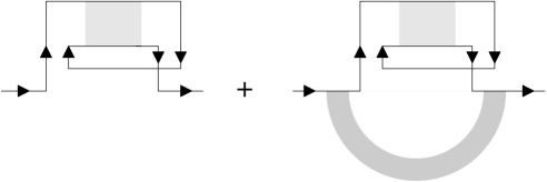
FIG. 2.: Diagrams contributing to the average single-particle Green’s function. The light-shaded regions represent a $D$-type cooperon mode, the dark-shaded one a nonsingular $\Pi_{A}^{{\rm d}0}$-ladder.

The sum of the former diagrams, which we call the $D$-type spin-singlet cooperon mode and denote by $S_{\alpha\gamma,\beta\delta}^{0}$, has the expression

$\displaystyle S^{0}=v^{2}\Pi_{0}/(1-v^{2}K\Pi_{0})$

with $K_{\alpha\gamma,\beta\delta}=\delta_{\alpha\beta}\delta_{\gamma\delta}G_{\alpha\alpha}^{0}G_{\gamma\gamma}^{0}$ and $\Pi_{0}\equiv\Pi_{D}^{{\rm c}0}$. Its large-$N$ limit is

$$S^{0}={\lambda^{2}\Pi_{0}\over-i\pi\nu\omega}+{\cal O}(1/N).$$ (55)

Similarly, the sum of all ladder diagrams built from $\Pi_{D}^{{\rm c}1}$-contractions, the $D$-type spin-triplet cooperon, is evaluated as

$$S^{1} = (1-\epsilon_{s})v^{2}\Pi_{1}/[1-(1-\epsilon_{s})v^{2}K\Pi_{1}]$$ (56)

$$= {\lambda^{2}\Pi_{1}\over\eta_{s}-i\pi\nu\omega}+{\cal O}(1/N)$$ (57)

where $\eta_{s}=4N\epsilon_{s}$ and $\Pi_{1}\equiv\Pi_{D}^{{\rm c}1}$. The dependence of $S^{1}$ on the parameter $\epsilon_{s}$ through the product $N\epsilon_{s}$ means that the breaking of spin-rotation invariance takes place on scales $\epsilon_{s}\sim 1/N$ and thus is very fast. This rapid crossover happens because the crossover scale is determined by the typical size of a symmetry-breaking matrix element in relation to the level spacing, which is $\nu^{-1}=\lambda\pi/4N$ for our choice of normalization.

Note that the expressions (55) and (57) are singular at $\omega=0=\eta_{s}$ even though the sums of ladder diagrams they represent are built from retarded Green’s functions only ($G^{+}G^{+}$ channel). This is a novel feature which does not occur for the standard Wigner-Dyson ensembles, where singular ladders exist only in the advanced-retarded (or $G^{-}G^{+}$) channel. The singularity in the present case comes about because the minus sign from $K_{\alpha\gamma,\alpha\gamma}=-1/\lambda^{2}$ is cancelled by a minus sign appearing in the definition of the contractions of type $D$, thereby turning an alternating (conditionally convergent) series into a divergent one.

The dark-shaded region appearing in the second diagram of Fig. 2 represents a $\Pi_{A}^{{\rm d}0}$-ladder. According to (45), the contractions of type $A$ come with an overall plus sign, so the minus signs now do not cancel, and the ladder sum is always finite. Computing the sum we find that this nonsingular $\Pi_{A}^{{\rm d}0}$-ladder renormalizes the first diagram in Fig. 2 by a factor of $1-(1-1+1-...)=1/(1+1)=1/2$. (We mention in passing that nonsingular ladders of this kind are the random-matrix analog of the single-impurity lines that appear in the context of the impurity diagram technique.)

To evaluate the first diagram of Fig. 2 we need the following sums:

$$\sum_{\beta}\left(\Pi_{D}^{{\rm c}0}\right)_{\alpha\beta,\beta\alpha}=-\sum_{\beta}\left(\Sigma_{x}\right)_{\beta\alpha}\left(\Sigma_{x}\right)_{\beta\alpha}=-1,$$ (58)

$$\sum_{\beta}\left(\Pi_{D}^{{\rm c}1}\right)_{\alpha\beta,\beta\alpha}=-\sum_{\beta}\left(\Sigma_{x}J_{k}\right)_{\beta\alpha}\left(J_{k}\Sigma_{x}\right)_{\beta\alpha}=+3.$$ (59)

We then obtain

$\displaystyle\langle g(\omega)\rangle=-i\pi\nu+i\pi\nu\left({3/2\over\eta_{s}-\pi i\nu\omega}-{1/2\over-\pi i\nu\omega}\right)+...,$

which agrees with the result stated at the beginning of the current subsection for $\eta_{s}=0$ (classes $C$ and $C$I) and $\eta_{s}\to\infty$ (classes $D$ and $D$III). For the classes $C$ and $D$, smooth corrections of higher order in $1/\omega$ are completely absent from the exact result of Sec. V A. This implies that all diagrams of higher order than the ones considered here must cancel each other, in these two cases. (The oscillatory correction $\sim A_{\beta}\omega^{-2/\beta}$ is nonanalytic in the expansion parameter $1/\omega$ and therefore remains invisible to all orders of perturbation theory.)

VI Slow Modes

In all previous Green’s function treatments of NS-systems the diagrams were enumerated by the number of Andreev reflections. Unfortunately, when the perturbation expansion is organized in that way, the vast number of possibilities to insert Andreev reflections into the diagrams generates a flood of terms which is hard to control, and as a result it is very easy to miss important contributions. The technical innovation made in the present paper is not to single out Andreev reflections but treat them on exactly the same footing as the processes of impurity scattering. This is possible by our dynamical assumptions ensuring that the quantum mechanical phase acquired during Andreev reflection, can be regarded as a random variable with zero mean. Our key technical step is the decomposition (53) which leads to an organization of the perturbation-theory diagrams by symmetry. In the preceding subsection we discussed how the contractions $\Pi_{D}^{{\rm c}0}$ and $\Pi_{D}^{{\rm c}1}$ generate singular geometric series of ladder diagrams. In the same way, every one of the other contractions gives rise to one singular ladder. These singular modes can be visualized as follows:

(60)

$$A{\rm-type}\;{\rm cooperon,}$$ (61)

(62)

$$A{\rm-type}\;{\rm diffuson,}$$ (63)

(64)

$$D{\rm-type}\;{\rm cooperon,}$$ (65)

(66)

$$D{\rm-type}\;{\rm diffuson.}$$ (67)

The dotted vertical lines represent both impurity scatterings and Andreev reflections, and they denote any one of the eight contractions $\Pi_{X}^{\rm xS}$ ($X=A,D$; ${\rm x}={\rm c,d}$; ${\rm S}=0,1$). The type of contraction is invariant within one ladder. The $A$-type modes are built from states of identical charge (two BdG-particles or two BdG-holes) propagating on opposite segments of the ladder, whereas the $D$-type modes are built from charge-reversed states (one particle and one hole). The former are singular in the $G^{+}G^{-}$ channel, the latter in the $G^{+}G^{+}$ (or $G^{-}G^{-}$) channel. The arrows on the Green’s function lines indicate the order in which single-particle states are visited. For the cooperon modes the order on both lines is the same, while for the diffuson modes it is reversed. In the limit $\omega=\eta_{s}=\eta_{t}=0$ (with $\eta_{t}=4N\epsilon_{t}$) all modes are singular, or massless. The $D$-type modes are made massive by frequency (or voltage) $\omega$ while the $A$-type modes are insensitive to such a perturbation. The $A$-type cooperon and the $D$-type diffuson are made massive by the breaking of time-reversal symmetry. Since a Green’s function line carries spin 1/2, the modes decompose into spin-singlet and spin-triplet ones. The spin-triplet modes are sensitive to spin-orbit scattering while the spin-singlet modes are not.

We wish to mention that there is some redundancy in our classification of modes, as the basic particle-hole symmetry (5) causes the existence of certain relations among the matrix elements of the Gorkov Green’s function $G^{\pm}(\omega)=(\omega\pm i\varepsilon-{\cal H})^{-1}$. In particular, the particle-particle and hole-hole matrix elements are related by

$$G_{\rm pp}^{\pm}(\omega)=-G_{\rm hh}^{\mp}(-\omega)^{\rm T}.$$ (68)

Similarly, $G_{\rm ph}^{\pm}(\omega)=-G_{\rm hp}^{\mp}(-\omega)^{\rm T}$. These identities transcribe into relations connecting the singular modes. For example, by using (68) on one of the Green’s function lines of the $D$-type cooperon, we can make this mode look like the $A$-type diffuson, at the expense of having to change the sign of one frequency $(\omega\to-\omega)$. In a similar way, the $D$-type diffuson is related to the $A$-type cooperon (again with a sign change in one of the frequencies). In spite of that, we prefer to treat the $A$- and $D$-type modes as separate entities. The main reason for doing so is that they respond differently to translations of the energy: while the $D$-type modes are made massive by shifting the energy, the $A$-type modes are not.

In the present paper we restrict our considerations to the ergodic (or zero-dimensional) limit. To go beyond, we should associate with each $A$-type and $D$-type mode a small momentum variable (“slow modes”) and sum over momenta. In this way, it will not be difficult to generalize our results beyond the ergodic limit.

VII Weak Localization

Having made a thorough analysis of the isolated Andreev quantum dot, we now turn to the discussion of the associated open system and its transport properties. To open up the dot in the simplest possible way, we couple it to a single lead with $2M$ open channels (the factor of 2 accounts for the spin degree of freedom), see Fig. 3.

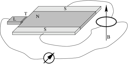
FIG. 3.: Andreev quantum dot (N) coupled to a single lead (L) via a tunnelling barrier (T). The flux loop on the right is introduced to adjust the difference of the order parameter phases of the superconducting regions (S) to the value $\phi_{1}-\phi_{2}=\pi$ (cf. the discussion of Sec. III).

The transmission of charge excitations from the lead to the interior of the dot is modelled by a set of (spin-independent) real hopping matrix elements $W_{\mu a}$, where the index $a=1,\dots,M$ ($\mu=1,\dots,N$) enumerates the channels carried by the lead (the sites of the dot). We assume $N\gg M\gg 1$. Let $g$ denote the conductance measured in units of $e^{2}/h$. To calculate $g$, we employ the Landauer-Büttiker formula as generalized to NS-systems by Takane and Ebisawa[25],

$$g=2\sum_{\tilde{a},\tilde{b}}|S_{\tilde{b}\tilde{a}}^{\rm hp}|^{2},$$ (69)

where the composite label $\tilde{a}=(a,s_{a})$ comprises the spin $s_{a}=\pm 1/2$ and the index $a$ of an open channel in the lead, and $S_{\tilde{b}\tilde{a}}^{\rm hp}$ denotes the scattering amplitude connecting a particle coming in in channel $\tilde{a}$ with a hole going out in channel $\tilde{b}$. The $S$-matrix is given by

$$S_{\tilde{b}\tilde{a}}^{\rm hp}=-2iW^{\rm T}_{\;\;b\mu}G_{(\mu,s_{b},{\rm h}),(\nu,s_{a},{\rm p})}W_{\nu a},$$ (70)

where

$\displaystyle G=(i\delta-{\cal H}+iWW^{\rm T})^{-1}$

is the Gorkov Green’s function evaluated at the chemical potential. Without loss of generality, we may assume the matrices $W=\{W_{\mu a}\}$ to be of the form

$$W_{\mu a}=\gamma^{1/2}\delta_{\mu a}\ (\mu=1,\dots,N;a=1,\dots,M).$$ (71)

The unitary transformation necessary to transform $W$ to the form (71) can be absorbed in the Hamiltonian $\cal{H}$ by the invariance properties of the random-matrix ensemble (16). Combining Eqs. (70) and (69) and making use of (71) we obtain

$$g=8\sum_{\mu s\mu^{\prime}s^{\prime}}\Gamma_{\mu}\left|G_{(\mu,s,{\rm h}),(\mu^{\prime},s^{\prime},{\rm p})}\right|^{2}\Gamma_{\mu^{\prime}},$$ (72)

where

$\displaystyle\Gamma_{\mu}=\left\{\begin{array}[]{ll}\gamma&\ {\rm for}\ \mu\leq M,\\ 0&\ {\rm else.}\end{array}\right.$

We are going to calculate this expression to leading order in the small parameters $1/N$, $M/N$ and next-to-leading order in $1/M$[26]. Owing to the presence of the BdG particle-hole degree of freedom, an analysis of Eq. (72) within the framework of plain diagrammatic perturbation theory turns out to involve a sizable number of diagrams. It is more efficient to pre-analyze (72) by means of a set of exact identities (Ward identities) before turning to diagrammatic methods. This calculation is detailed in Appendix A. Here we restrict ourselves to a presentation of the results and their interpretation in terms of semiclassical trajectories.

Schematically, the conductance can be represented as:

$$g=\begin{minipage}{199.16928pt} \psfig{height=22.76228pt} \end{minipage}$$ (73)

where the wavy lines stand for the quantities $\{\Gamma_{\mu}\}$, the shaded region denotes the singular $A$-type diffuson mode introduced in Sec. VI,

$\displaystyle\psfig{height=17.07182pt},$

and a summation over indices is understood. The WL-building block represents a quantum interference correction (the NS-analog of the well-known weak localization correction for normal metals) to the classical conductance. In contrast with the pure N-case, however, two qualitatively different processes contribute to the weak localization correction for the Andreev dot:

.

Here the $A$($D$)-block is due to the presence of singular $A$($D$)-type modes. Whereas the $A$-type contribution resembles the standard weak localization correction known from normal metals, the $D$-term does not have any analog in pure N-systems and is of a different nature. In the following we discuss separately the classical conductance (the first diagram in (73)), the $A$-type correction, and the $D$-type correction.

Classical conductance: Qualitatively speaking, the conductance is given by

$$g=\left|\sum_{i}A_{i}\right|^{2},$$ (74)

where $A_{i}$ is the amplitude to traverse a certain scattering sequence (indexed by $i$) connecting an incoming particle channel with an outgoing hole channel. The classical value of the conductance, $g_{0}$, is obtained by evaluating the incoherent sum

$\displaystyle g_{0}=\sum_{i}\left|A_{i}\right|^{2}.$

Quantitatively, we obtain

$\displaystyle g_{0}=2MT,$

where the transmission coefficient $T$ is the probability for an electron incident from the lead to enter the dot instead of being reflected back into the lead[27]. This result is easy to understand. By the ergodicity of our system, an electron leaves the dot with equal ($1/2$) probability as a particle or as a hole. In the latter case, two elementary charges are transferred across the entire system. Thus the dimensionless conductance per channel is $2\times 1/2\times T=T$. Multiplying by the number of channels we get $g_{0}=2MT$.

$A$-type corrections: Weak localization corrections to the classical conductance originate from the phase-coherent contributions of nonidentical paths to the sum of amplitudes (74). In the case of the $A$-type correction, such contributions are due to pairs of paths that differ by a sequence of scattering events traversed in opposite directions as is indicated in Fig. 4.

FIG. 4.: Pair of semiclassical paths contributing to the $A$-type weak localization process.

The sum of these “maximally crossed” segments of pairs of paths is represented by the building block $A$ in (73). More specifically,

$\displaystyle\begin{minipage}{227.62204pt} \psfig{height=45.52458pt} \end{minipage}+\dots,$

where the shaded region represents an $A$-type cooperon, the subscript ‘t’ means that the external arrows are shown merely for the sake of clarity but do not contribute to the $A$-block as such, and the dots stand for diagrams of a more complex structure that have to be taken into account to obtain a result consistent with unitarity. It is the presence of these unitarity-preserving contributions that renders the calculation of the $A$-block within plain diagrammatic perturbation theory lengthy. The alternative computational scheme presented in Appendix A yields

$\displaystyle\delta g^{A}=\frac{M}{2}T^{2}\left(\frac{1}{MT+\eta_{t}}-\frac{3}{MT+\eta_{s}+\eta_{t}}\right),$

where the parameters $\eta_{s}=4N\epsilon_{s}$ and $\eta_{t}=4N\epsilon_{t}$ are the scaled symmetry-breaking parameters of our model.

$D$-type corrections: A pair of paths contributing to the $D$-type weak localization process is shown in Fig. 5.

FIG. 5.: Pair of semiclassical paths contributing to the $D$-type weak localization process. The triangles represent Andreev reflections.

Note that the self-intersecting loop must contain a nonvanishing even number of Andreev reflections (the figure displays the simplest possible case of just two Andreev events). We note in passing that the $A$-type loop shown in Fig. 4 may contain Andreev reflections, too (for this reason we said that the NS $A$-type correction is analogous to, though not identical with, the normal weak localization correction), their presence is just not imperative like in the $D$-case. Clearly, the $D$-type correction does not have any analog in normal metals. Note also that the closed loop in Fig. 5 involves only one of the two paths. This shows that the existence of the $D$-type process is essentially due to the nontrivial behavior of the single-particle Green’s function. The same mechanism of quantum coherence at the single-particle level was responsible for the correction to the single-particle density of states discussed in Sec. V B.

In diagrammatic language, the loop insertion in Fig. 5 is represented by

$\displaystyle\begin{minipage}{227.62204pt} \psfig{height=71.13188pt} \end{minipage}+\dots,$

where the shaded region now represents a $D$-type cooperon mode and the dots stand for a set of unitarity-preserving counter diagrams. The quantitative analysis yields

$\displaystyle\delta g^{D}=(1-T)\left(1-\frac{3MT}{MT+\eta_{s}}\right).$

A striking feature of this expression is its insensitivity to the breaking of time-reversal symmetry: the $D$-type weak localization correction for NS-systems survives the application of external magnetic fields[28]. Collecting terms we obtain the final result

$$\langle g\rangle=2MT+(1-T)\left(1-\frac{3MT}{MT+\eta_{s}}\right)$$ (75)

$$\hskip 14.22636pt+\frac{M}{2}T^{2}\left(\frac{1}{MT+\eta_{t}}-\frac{3}{MT+\eta_{s}+\eta_{t}}\right)$$ (76)

$$\hskip 113.81102pt+{\cal O}(1/M,M/N)$$ (77)

for the dimensionless mean conductance of our system at zero bias. We see that the $D$-type correction is zero for $T=1$, while the $A$-type correction vanishes in the limit $T\to 0$, with $MT$ held fixed. From what has been said about the $D$-type modes, we expect the $D$-type correction to disappear at finite bias. Detailed analysis shows that the crossover scale for this to happen is determined by $\nu\omega\sim MT$.

VIII Universal Conductance Fluctuations

The conductance fluctuations of normal-conducting systems[29] have been studied extensively. They are independent of system size and strength of the disorder and depend only on symmetry. The latter dependence can be summarized by saying that ${\rm var}(g)$ is proportional to the number of massless modes for a given universality class. When all symmetries are broken, the $A$-type spin-singlet diffuson is the only mode which is massless. As we switch off the spin-orbit interaction, the $A$-type spin-triplet diffuson modes become massless, too, which increases ${\rm var}(g)$ by a factor of four. If in addition time reversal is a good symmetry, the cooperon modes become massless, thereby increasing ${\rm var}(g)$ by yet another factor of two.

The NS-systems considered in the present paper are expected[30] to show conductance fluctuations that are qualitatively similar to those of N-systems. To calculate the variance, we may use an extension of the diagrammatic method described in the previous section or, alternatively, we may map our random-matrix model on a zero-dimensional field theory of the nonlinear $\sigma$ model type. In the present paper neither of these methods will be used. Instead, we will turn to another approach, which is restricted to the strong-coupling limit $T=1$ but has the great advantage of being very simple.

The symmetry properties of the $S$-matrix derive from the symmetries of the Hamiltonian by exponentiation. As before, let $M$ denote the number of channels in the lead, not counting spin and particle-hole degeneracy. By the considerations of Sec. II the $S$-matrix may be regarded as an element of the symmetric space ${\rm SO}(4M)$ for class $D$, ${\rm Sp}(2M)$ for $C$, ${\rm SO}(4M)/{\rm U}(2M)$ for $D$III, and ${\rm Sp}(2M)/{\rm U}(M)$ for $C$I. We will refer to these spaces as “$S$-matrix manifolds” for short. Let $A=(a,s,\sigma)$ $(a=1,...,M;s=\pm 1/2;\sigma={\rm p,h})$ be a composite index. From the definition of the transmission coefficient $T$ as a “sticking probability” [31] we have $T=1-|\langle S_{AA}\rangle|^{2}+{\cal O}(1/MT)$. Therefore $T=1$ implies an $S$-matrix with vanishing ensemble average, which means that $S$ can be taken to be uniformly distributed on its $S$-matrix manifold.

A Class $C$

For the symmetry classes $C$ and $C$I the $S$-matrix operates on the tensor product of channel space and particle-hole space, while spin is accounted for by multiplication of the conductance by a factor of two. Recall the definition of the symplectic group ${\rm Sp}(2M)$ by

$${U^{-1}}^{\dagger}=U={\cal C}{U^{-1}}^{\rm T}{\cal C}^{-1}$$ (78)

where ${\cal C}={\bf 1}_{M}\otimes i\sigma_{y}$. In keeping with the above, we take the $S$-matrix $S\equiv U$ for class $C$ to be uniformly distributed on ${\rm Sp}(2M)$. In other words, ensemble averages $\langle...\rangle$ are computed by integrating with respect to the Haar measure $dU$:

$\displaystyle\langle f(U)\rangle=\int_{{\rm Sp}(2M)}f(U)dU.$

The canonical projection of ${\rm Sp}(2M)$ onto the coset space ${\rm Sp}(2M)/{\rm U}(M)$ by $U\mapsto UU^{\rm T}$ turns the Haar measure of the former into the invariant (or uniform) measure of the latter. Therefore, ensemble averages for class $C$I can be obtained from

$\displaystyle\langle f(S)\rangle_{C{\rm I}}=\langle f(UU^{\rm T})\rangle.$

Because the Haar integral is invariant under left and right translations,

$\displaystyle\int_{{\rm Sp}(2M)}f(U_{L}UU_{R})dU=\int_{{\rm Sp}(2M)}f(U)dU,$

the defining equations for ${\rm Sp}(2M)$ lead to

$$\langle U_{AB}\rangle = 0,$$ (79)

$$\langle U_{AB}^{\vphantom{*}}U_{CD}^{*}\rangle = \delta_{AC}\delta_{BD}/2M,$$ (80)

$$\langle U_{AB}U_{CD}\rangle = {\cal C}_{AC}{\cal C}_{BD}/2M.$$ (81)

To compute the ensemble average of a product of two $U$’s and two ${U^{*}}$’s we note that if $\psi_{A}\in V$ are the components of a vector transforming according to the fundamental representation of ${\rm Sp}(2M)$, there exist only two independent invariants on $V\otimes V^{*}\otimes V\otimes V^{*}$, namely $\sum\psi_{A}^{\vphantom{*}}\psi_{A}^{*}\psi_{B}^{\vphantom{*}}\psi_{B}^{*}$ and $\sum{\cal C}_{AB}{\cal C}_{CD}\psi_{A}\psi_{B}\psi_{C}^{*}\psi_{D}^{*}$. Using this elementary group-theoretical fact we obtain

$$\langle U_{A_{1}B_{1}}^{\vphantom{*}}U_{C_{1}D_{1}}^{*}U_{A_{2}B_{2}}^{\vphantom{*}}U_{C_{2}D_{2}}^{*}\rangle$$ (82)

$$= {2M-1\over 2M(2M+1)(2M-2)}\Bigl{[}\delta_{A_{1}C_{1}}\delta_{A_{2}C_{2}}\delta_{B_{1}D_{1}}\delta_{B_{2}D_{2}}$$ (85)

$$\qquad\qquad\qquad\qquad\qquad+\delta_{A_{1}C_{2}}\delta_{A_{2}C_{1}}\delta_{B_{1}D_{2}}\delta_{B_{2}D_{1}}$$

$$\qquad\qquad\qquad\qquad\qquad+{\cal C}_{A_{1}A_{2}}{\cal C}_{C_{1}C_{2}}{\cal C}_{B_{1}B_{2}}{\cal C}_{D_{1}D_{2}}\Bigr{]}$$

$$- {1\over 2M(2M+1)(2M-2)}\Bigl{[}\delta_{A_{1}C_{1}}\delta_{A_{2}C_{2}}\delta_{B_{1}D_{2}}\delta_{B_{2}D_{1}}$$ (89)

$$\qquad\qquad\qquad\qquad\qquad+\delta_{A_{1}C_{2}}\delta_{A_{2}C_{1}}\delta_{B_{1}D_{1}}\delta_{B_{2}D_{2}}$$

$$\qquad\qquad+(\delta_{A_{1}C_{1}}\delta_{A_{2}C_{2}}-\delta_{A_{1}C_{2}}\delta_{A_{2}C_{1}}){\cal C}_{B_{1}B_{2}}{\cal C}_{D_{1}D_{2}}$$

$$\qquad\qquad+{\cal C}_{A_{1}A_{2}}{\cal C}_{C_{1}C_{2}}(\delta_{B_{1}D_{1}}\delta_{B_{2}D_{2}}-\delta_{B_{1}D_{2}}\delta_{B_{2}D_{1}})\Bigr{]}.$$

The numerical coefficients in this expression are determined by summing over any two pairs of equal indices and then comparing the results to (80) using the relations (78). Equation (89) entails

$\displaystyle\sum_{AB}\langle U_{{\rm p}A}^{\vphantom{*}}U_{{\rm h}A}^{\vphantom{*}}U_{{\rm p}B}^{*}U_{{\rm h}B}^{*}\rangle=(2M+1)^{-1},$

which can be used to compute the weak localization correction for class $C$I. Summing over initial and final (or particle and hole) channels, we get $\langle{\rm Tr}S^{\rm ph}S^{\dagger{\rm hp}}\rangle_{C{\rm I}}=M^{2}/(2M+1)$ which yields $\delta g=-1$ in agreement with (77). To calculate the conductance fluctuations for class $C$, we deduce from (89)

$\displaystyle\langle\left({\rm Tr}S^{\rm ph}S^{\dagger{\rm hp}}\right)^{2}\rangle={M^{2}\over 4}+{1\over 8}+{\cal O}(M^{-1}).$

Subtracting the square of the first moment and multiplying by a factor of $4\times 4$ for charge and spin, we get ${\rm var}(g)=2$.

B Class $D$

The symmetry class $D$ can be treated by direct transcription from class $C$, the only difference being the way the spin enters. The $S$-matrix now operates on the full tensor product of channel space, particle-hole space and spin space. The $S$-matrix manifold for $D$ is isomorphic to the orthogonal group ${\rm SO}(4M)$, and is defined by (78) with ${\cal C}={\bf 1}_{M}\otimes\sigma_{x}\otimes{\bf 1}$. Equations (80) remain formally unchanged except for the replacement $2M\to 4M$. The projection $U\mapsto U\tau U^{\rm T}\tau^{-1}$ with $\tau={\bf 1}_{M}\otimes{\bf 1}\otimes i\sigma_{y}$ takes the Haar measure of ${\rm SO}(4M)$ into the invariant measure of ${\rm SO}(4M)/{\rm U}(2M)$. Ensemble averages are given by

$$\langle f(S)\rangle_{D{\rm III}} = \langle f(U\tau U^{\rm T}\tau^{-1})\rangle,$$ (90)

$$\langle f(U)\rangle = \int_{{\rm SO}(4M)}f(U)dU.$$ (91)

The ensemble average of a product of four $U^{\prime}s$ is

$$\langle U_{A_{1}B_{1}}^{\vphantom{*}}U_{C_{1}D_{1}}^{*}U_{A_{2}B_{2}}^{\vphantom{*}}U_{C_{2}D_{2}}^{*}\rangle$$ (92)

$$= {4M+1\over 4M(4M-1)(4M+2)}\Bigl{[}\delta_{A_{1}C_{1}}\delta_{A_{2}C_{2}}\delta_{B_{1}D_{1}}\delta_{B_{2}D_{2}}$$ (95)

$$\qquad\qquad\qquad\qquad\qquad+\delta_{A_{1}C_{2}}\delta_{A_{2}C_{1}}\delta_{B_{1}D_{2}}\delta_{B_{2}D_{1}}$$

$$\qquad\qquad\qquad\qquad\qquad+{\cal C}_{A_{1}A_{2}}{\cal C}_{C_{1}C_{2}}{\cal C}_{B_{1}B_{2}}{\cal C}_{D_{1}D_{2}}\Bigr{]}$$

$$- {1\over 4M(4M-1)(4M+2)}\Bigl{[}\delta_{A_{1}C_{1}}\delta_{A_{2}C_{2}}\delta_{B_{1}D_{2}}\delta_{B_{2}D_{1}}$$ (99)

$$\qquad\qquad\qquad\qquad\qquad+\delta_{A_{1}C_{2}}\delta_{A_{2}C_{1}}\delta_{B_{1}D_{1}}\delta_{B_{2}D_{2}}$$

$$\qquad\qquad+(\delta_{A_{1}C_{1}}\delta_{A_{2}C_{2}}+\delta_{A_{1}C_{2}}\delta_{A_{2}C_{1}}){\cal C}_{B_{1}B_{2}}{\cal C}_{D_{1}D_{2}}$$

$$\qquad\qquad+{\cal C}_{A_{1}A_{2}}{\cal C}_{C_{1}C_{2}}(\delta_{B_{1}D_{1}}\delta_{B_{2}D_{2}}+\delta_{B_{1}D_{2}}\delta_{B_{2}D_{1}})\Bigr{]}.$$

The remaining calculations are the same as before. We obtain $\delta g=+1/2$ for class $D$III, and ${\rm var}(g)=1/2$ for class $D$.

C Conjecture for $C$I and $D$III

For N-systems the breaking of time-reversal symmetry is known to reduce ${\rm var}(g)$ by a factor of two, while the breaking of spin-rotation invariance causes a reduction by a factor of four. As was said earlier, this pattern is explained by the observation that ${\rm var}(g)$ simply counts the number of massless modes in each universality class. From our experience with diagrammatic perturbation theory of the model (16,70) we expect the same principle to be operative here, i.e. we expect ${\rm var}(g)$ to be still determined by the number of massless modes. Indeed, the conductance fluctuations for the classes $C$ and $D$ are seen to be bigger than the corresponding fluctuations for N-systems by a factor of eight. To understand this, we note that there is a trivial enhancement by a factor of $2^{2}=4$ due to the transfer of two elementary charges in an Andreev reflection. The other factor of two can be interpreted as telling us that the number of massless modes a priori is twice as large: for every $A$-type mode, which is already present in the N-system, there exists an extra $D$-type (or BdG particle-hole) mode in the NS-system, see Sec. VI. By extrapolation we are led to the following conjecture:

$\displaystyle{\rm var}(g)=\left\{\matrix{4&\quad(C{\rm I}),\cr 2&\quad(C),\cr 1&\quad(D{\rm III}),\cr 1/2&\quad(D),\cr}\right.$

which differs from the result of Brouwer and Beenakker[30] who found the size of the conductance fluctuations to depend only weakly on whether time-reversal symmetry is broken or not. Note however that their result applies to a different situation than the one considered here (In their case the superconducting order parameter is homogeneous in space for class $C$I).

IX Conclusions

In this paper we have initiated the study of a special family of NS-systems where the spatial variation of the superconducting order parameter is such that the Andreev phase shift averages to zero along a typical semiclassical single-electron trajectory. We find such systems particularly interesting because the proximity effect is inoperative and quasiparticle states exist right at the chemical potential. Disorder or dynamically generated chaos mixes the states and leads to a novel and universal type of level statistics within an energy window whose size is determined by the frequency of Andreev reflection. By classifying systems according to their symmetries we identified four universality classes, denoted by $C$, $C$I, $D$, and $D$III. Time reversal is a good (broken) symmetry for $C$I and $D$III ($C$ and $D$), while spin is conserved (not conserved) for $C$ and $C$I ($D$ and $D$III). For each universality class the joint probability distribution of the quasiparticle energy levels was given in closed form. The $n$-level correlation functions for the classes $C$ and $D$ were calculated by the mapping onto a free Fermi gas on a half-line with Dirichlet and Neumann boundary conditions at the origin. The joint probability distributions of the levels for $C$I and $D$III were transformed into those of the Laguerre Orthogonal and Laguerre Symplectic Ensembles, whose level statistics has been worked out completely (albeit with a minor computational error) by Nagao and Slevin.

To calculate the transport properties of open systems in the zero-dimensional limit, we formulated a random-matrix model and treated it using a variant of the impurity diagram technique. An important feature we pointed out was the doubling of the number of low-energy modes in comparison with conventional normal-conducting systems. For every $A$-type mode, i.e. for every BdG particle-particle (or hole-hole) spin-singlet or spin-triplet diffuson or cooperon, there exists precisely one corresponding BdG particle-hole or $D$-type mode. The weak localization correction to the average conductance for an NSS-geometry was calculated as a function of the “sticking probability” $T$ and two perturbations breaking time-reversal symmetry and spin-rotation invariance. The technically more involved task of calculating the variance of the fluctuating conductance was carried out only for $T=1$ and the universality classes $C$ and $D$, by using an $S$-matrix formalism á la Mello. We found ${\rm var}(g)$ to be enhanced by a factor of two relative to the rule ${\rm var}(g_{\rm NS})=4{\rm var}(g_{\rm N})$. We attribute this enhancement to the doubling of low-energy modes by the coupling to the superconductor. Let us emphasize that the effects we have studied are universal (in the ergodic limit) and are independent of such microscopic detail as the NS-barrier transmittency.

Clearly, the present paper constitutes only a first step into a new and exciting research area of mesoscopic physics, and much more is yet to be done. Some of the open problems are the following. (i) We have shown how to solve the level statistics problem for each universality class but more generally one might also be interested in the crossover between classes. Here the crossovers $C{\rm I}\to C$ and $D{\rm III}\to D$ look amenable to analytical techniques, since the level statistics for $C$ and $D$ (just as for the Gaussian Unitary Ensemble) maps on a free Fermi gas problem. (ii) Our results for the level statistics are restricted to an energy range proportional to the inverse mean time spent between successive Andreev reflections. To access the short-time or high-energy regime beyond the crossover scale, our maximum-entropy ensembles need to be modified by allowing for different variances of the random pairing and normal matrix elements. (iii) Although we have outlined the semiclassical interpretation of the $D$-type (or particle-hole) modes, a more detailed discussion of their role in semiclassical periodic-orbit theory would certainly be desirable. (iv) We need to extend our results for the universal conductance fluctuations to the classes $C$I and $D$III and to arbitrary $T$. (v) While the zero-dimensional (or ergodic) limit is adequately described by the maximum-entropy ansatz, the diffusive and ballistic regimes necessitate a more detailed modelling. In particular, the nonrandom nature of the magnitude of the pairing field will make itself felt at short times. It is an open technical problem how to deal analytically with the phase randomness of Hamiltonian matrix elements when their magnitude is to be kept fixed. (vi) We have concentrated on an NS-geometry that is particularly easy to treat but future work will have to include other geometries. (vii) Last but not least, we need to address the nontrivial question: how large is the effect of residual Coulomb interactions on the $D$-type modes? There is no doubt that the short-time physics can be adequately described in a simple independent-quasiparticle picture, but at large times the coherence between particles and holes will get cut off by Coulomb blockade and other correlation effects. The question is what is the time scale where this happens.

We shall end on a mathematical note. According to Cartan, there exist eleven large families of symmetric spaces. Those of type II are the compact unitary, orthogonal and symplectic Lie groups $(A,B,C,D)$. The large families of type-I symmetric spaces are denoted by $A$I, $A$II, $A$III, $BD$I, $C$I, $C$II, and $D$III. The standard Wigner-Dyson universality classes derive from $A$ (GUE), $A$I (GOE), and $A$II (GSE), while the universality classes of a massless Dirac particle derive from $A$III (chGUE), $BD$I (chGOE), and $C$II (chGSE). As we have shown, the new universality classes found in mesoscopic NS-systems exhaust the remaining large families of symmetric spaces except for $B$ (the orthogonal group in odd dimensions), which does not occur. Thus, if we group $B$ together with $D$, there is a bijection between the known universality classes of disordered single-particle systems and the large families of symmetric spaces. We consider this to be a strong indication that no other universality classes will be found, since any additional universality class would exceed Cartan’s scheme and therefore would have to be of a different nature.

Acknowledgment. This work was supported in part by the Deutsche Forschungsgemeinschaft, SFB 341.

A Conductance and Ward Identities

In this appendix we elaborate on the calculation of the weak localization correction to the conductance, Eq. (77). Owing to the presence of the BdG particle-hole degree of freedom, this calculation turns out to be much more involved than in pure N-systems. For this reason we prefer to control the diagrammatic expansion by means of exact algebraic relationships. The basic concepts used in this appendix have been introduced in the seminal paper[32].

To begin with, we recapitulate two Ward identities that will play a crucial role in what follows. Let us write the average retarded Green’s function as $\langle G_{\alpha,\alpha^{\prime}}\rangle=\delta_{\alpha,\alpha^{\prime}}(-\Sigma_{\mu}+i\Gamma_{\mu})^{-1}=:\delta_{\alpha,\alpha^{\prime}}G_{\mu}$, where $\alpha=(\mu,s,q)$ is a composite index accounting for the site ($\mu)$, spin ($s$) and particle-hole ($q={\rm p,h}$) degrees of freedom. (After averaging, the Green’s function depends only on the site index.) The first Ward identity is immediate from the definitions and reads

$$G_{\mu}^{\vphantom{*}}G_{\mu}^{*}=-\Delta G_{\mu}\left(-\Delta\Sigma_{\mu}+2i\Gamma_{\mu}\right)^{-1},$$ (A1)

where $G_{\mu}^{*}$ is the average advanced Green’s function, $\Delta G_{\mu}=G_{\mu}-G_{\mu}^{*}$ and $\Delta\Sigma_{\mu}=\Sigma_{\mu}-\Sigma_{\mu}^{*}$. A second and less trivial Ward-identity[32] relates the self energy $\Sigma$ to the so-called irreducible two-particle vertex $U$:

$$\Delta\Sigma_{\mu}=\sum_{\alpha^{\prime}}U_{\alpha,\alpha^{\prime}}\Delta G_{\mu^{\prime}}.$$ (A2)

The irreducible vertex $U$ is defined as the set of all truncated four-point functions that cannot be cut by just cutting two average Green’s functions, i.e.

$\displaystyle U=\begin{minipage}{142.26378pt} \psfig{height=19.91684pt} \end{minipage}.$

In the following we focus on the analysis of the auxiliary quantity

$\displaystyle\Phi_{\alpha}=\sum_{\alpha^{\prime};q^{\prime}={\rm p}}\langle\left|G_{\alpha,\alpha^{\prime}}\right|^{2}\rangle\Gamma_{\mu^{\prime}}.$

¿From this the mean conductance is obtained as (cf. (72))

$$\langle g\rangle=8\sum_{\alpha;q={\rm h}}\Gamma_{\mu}\Phi_{\alpha}.$$ (A3)

We start from the ansatz

$$\Phi_{\alpha}=\Delta G_{\mu}\Big{[}c+c_{s}(-)^{s}+c_{q}(-)^{q}+c_{sq}(-)^{s+q}+$$ (A4)

$$\hskip 28.45274pt+\Gamma_{\mu}\left(d+d_{s}(-)^{s}+d_{q}(-)^{q}+d_{sq}(-)^{s+q}\right)\Big{]}.$$ (A5)

(Although other expressions involving arbitrary functions of $\Gamma_{\mu}$ seem possible, this formula does represent the most general starting point. Equation (71) yields $\sum_{\mu}\Gamma_{\mu}^{n}=\gamma^{n-1}\sum_{\mu}\Gamma_{\mu}$, so it is sufficient to start from an expression that is linear in the coefficients $\Gamma_{\mu}$.) The quantity $\Phi$ satisfies Dyson’s equation[32]

$$\left(\Delta\Sigma_{\mu}-2i\Gamma_{\mu}\right)\Phi_{\alpha}=\Delta G_{\mu}\left(\Gamma_{\mu}\delta_{q{\rm p}}+\sum_{\alpha^{\prime}}U_{\alpha,\alpha^{\prime}}\Phi_{\alpha^{\prime}}\right)\hskip 8.5359pt(*),$$ (A6)

where use of the identity (A1) has been made. To fix the coefficients $c,\dots,d,\dots$ we subject Eq. (A6) to various summation procedures. For example, by taking the sum $\sum_{\alpha}(*)$ and then using the second Ward identity (A2), we obtain

$$c+\gamma d=-1/4i.$$ (A7)

Seven more equations for the remaining coefficients are generated by performing the summations $\sum_{\alpha}(-)^{s}(*)$, $\sum_{\alpha}(-)^{q}(*)$, $\sum_{\alpha}(-)^{s+q}(*)$, $\sum_{\alpha}\Gamma_{\mu}(*)$, $\sum_{\alpha}\Gamma_{\mu}(-)^{s}(*)$, $\sum_{\alpha}\Gamma_{\mu}(-)^{q}(*)$ and $\sum_{\alpha}\Gamma_{\mu}(-)^{s+q}(*)$. The outcome of all this may be cast in the form of a matrix equation

$$\left(\begin{array}[]{cc}A&B\\ C&D\end{array}\right)\left(\begin{array}[]{c}\vec{c}\\ \vec{d}\end{array}\right)=-2a_{1}\left(\begin{array}[]{c}\vec{u}\\ \vec{v}\end{array}\right),$$ (A8)

where $\vec{c}^{\rm T}=(c_{s},c_{q},c_{sq})$, $\vec{d}^{\rm T}=(d,d_{s},d_{q},d_{sq})$, $\vec{u}^{\rm T}=(0,1,0)$, $\vec{v}^{\rm T}=(0,0,\gamma,0)$, and $a_{1}=\sum_{\mu}\Gamma_{\mu}\Delta G_{\mu}$. Fortunately, it is easy to invert the $7\times 7$ matrix appearing in this equation. By construction, the coefficients appearing in the subblock $A(B,C,D)$ involve summations over the index $\alpha$ that do not (do) contain matrix elements $\Gamma_{\mu}$. Since $\sum_{\alpha}\dots\sim{\cal O}(N)$, whereas $\sum_{\alpha}\Gamma_{\mu}\dots\sim{\cal O}(M)$, the coefficients appearing in $A$ exceed those in the remaining subblocks by a large factor of ${\cal O}(N/M)$. We thus conclude

$$\left(\begin{array}[]{cc}A&B\\ C&D\end{array}\right)^{-1}\simeq\left(\begin{array}[]{cc}0&0\\ 0&D^{-1}\end{array}\right)\Rightarrow\vec{c}\simeq 0,\ \vec{d}\simeq D^{-1}\vec{v}.$$ (A9)

The matrix $D$ can easily be inverted as it is already of diagonal form. Combining Eqs. (A3), (A7) and (A9), we obtain

$$\langle g\rangle=16a_{1}\left(-\frac{1}{4i}-\frac{2\gamma^{2}a_{1}}{4\gamma c_{1}-8i\gamma^{2}a_{1}-\overline{U}}\right),$$ (A10)

where $c_{1}=\sum_{\mu}\Gamma_{\mu}\Delta G_{\mu}\Delta\Sigma_{\mu}$ and

$\displaystyle\overline{U}=\sum_{\alpha,\alpha^{\prime}}\Gamma_{\mu}\Delta G_{\mu}(-)^{q}U_{\alpha,\alpha^{\prime}}\Gamma_{\mu^{\prime}}\Delta G_{\mu^{\prime}}(-)^{q^{\prime}}.$

We next decompose the self energy according to $\Sigma_{\mu}=-i/\lambda+\delta\Sigma_{\mu}$ into a leading order contribution plus a correction term $\delta\Sigma_{\mu}$ of ${\cal O}(1/M)$. Anticipating that the terms $\delta\Sigma_{\mu}$ and $\overline{U}$ are of the same order, we obtain the preliminary result

$$\langle g\rangle=2MT+2MT\frac{\lambda-\gamma}{\lambda(\lambda+\gamma)}{\rm Im}\overline{\delta\Sigma}+\frac{1}{2(\lambda+\gamma)^{2}}\overline{U}+$$ (A11)

$$\hskip 14.22636pt+{\cal O}(1/M),$$ (A12)

where $\overline{\delta\Sigma}=(M\gamma)^{-1}\sum_{\mu}\Gamma_{\mu}\delta\Sigma_{\mu}$. We next analyze the building blocks $\overline{\delta\Sigma}$ and $\overline{U}$ by diagrammatic methods. Because Eq. (A12) is based on Ward identities, it automatically incorporates the condition of unitarity. As a consequence, the following calculation is much simpler than a direct diagrammatic analysis of Eq. (72).

To leading order in $M^{-1}$, the self-energy correction $\overline{\delta\Sigma}$ is given by

$$\overline{\delta\Sigma}=\frac{1}{4M\gamma}\sum_{\alpha}\Gamma_{\mu}\begin{minipage}{199.16928pt} \psfig{height=51.21504pt} \end{minipage},$$ (A13)

where the light-(dark-)shaded region represents a $D$–type cooperon mode (a non–singular $\Pi_{A}^{d0}$–ladder). Evaluation of the diagrams yields (cf. the explanation in connection with Fig.2)

$${\rm Im}\overline{\delta\Sigma}={\lambda(\lambda-\gamma)\over 2(\lambda+\gamma)}\left[\frac{1}{MT}-\frac{3}{MT+\eta_{s}}\right].$$ (A14)

The dominant contribution to the vertex correction $\overline{U}$ results from an $A$–type cooperon:

$$\overline{U}=\sum_{\alpha,\alpha^{\prime}}(-)^{q}\Gamma_{\mu}\Delta G_{\mu}\begin{minipage}{71.13188pt} \psfig{height=39.83368pt} \end{minipage}\Delta G_{\mu^{\prime}}\Gamma_{\mu^{\prime}}(-)^{q^{\prime}}=$$ (A15)

$$\hskip 14.22636pt=4\lambda\gamma TM\left(\frac{1}{MT+\eta_{t}}-\frac{3}{MT+\eta_{s}+\eta_{t}}\right).$$ (A16)

(A17)

By combining Eqs. (A12), (A14) and (A17), and using the expression for the transmission coefficient $T=4\lambda\gamma/(\lambda+\gamma)^{2}$, we arrive at the final result given in Sec. VII.

REFERENCES

- [1] E.P. Wigner, Proc. Cambrdg. Phil. Soc. 47, 790 (1951); Ann. Math. 67, 325 (1958).
- [2] F.J. Dyson, J. Math. Phys. 3, 140, 1199 (1962).
- [3] K.B. Efetov, Adv. Phys. 32, 53 (1983).
- [4] J.J.M. Verbaarschot and I. Zahed, Phys. Rev. Lett. 70, 3853 (1993); J.J.M. Verbaarschot, Phys. Rev. Lett. 72, 2531 (1994).
- [5] R. Gade, Nucl. Phys. B398, 499 (1993); T. Nagao and K. Slevin, Phys. Rev. Lett. 70, 635 (1993).
- [6] R. Oppermann, Physica A167, 301 (1990).
- [7] K. Slevin, J.L. Pichard, and P.A. Mello, submitted to Journal de Physique.
- [8] A.F. Andreev, Zh. Eksp. Teor. Fiz. 46, 1823 (1964) [Sov. Phys. JETP 19, 1228 (1964)].
- [9] A. Altland and M.R. Zirnbauer, cond-mat/9508026.
- [10] R. Balian and E. Brézin, Nuov. Cim. 64B, 37 (1969).
- [11] S. Helgason, Differential geometry, Lie groups, and symmetric spaces, Academic Press, New York 1978.
- [12] A. Kastalsky, A.W. Kleinsasser, L.H. Greene, R. Bhat, F.P. Milliken, and J.P. Harbison, Phys. Rev. Lett. 67, 3026 (1991).
- [13] B.J. van Wees, P. de Vries, P. Magnée, and T.M. Klapwijk, Phys. Rev. Lett. 69, 690 (1992).
- [14] C.W.J. Beenakker, in Mesoscopic Quantum Physics, E. Akkermans, G. Montambaux, and J.-L. Pichard, eds., North-Holland, Amsterdam 1996; cond-mat/9406083.
- [15] A.F. Andreev, Zh. Eksp. Teor. Fiz. 49, 655 (1965) [Sov. Phys. JETP 22, 455 (1966)].
- [16] I.O. Kulik, Zh. Eksp. Teor. Fiz. 57, 1745 (1969) [Sov. Phys. JETP 30, 944 (1970)].
- [17] B. Sutherland, J. Math. Phys. 12, 246 (1971); see also B.D. Simons, P.A. Lee and B.L. Altshuler, Phys. Rev. Lett. 72, 64 (1994).
- [18] M.A. Olshanetsky and A.M. Perelomov, Phys. Rep. 94, 313 (1983).
- [19] M.R. Zirnbauer and F.D.M. Haldane, Phys. Rev. B52, 8729 (1995).
- [20] A. Luther and I. Peschel, Phys. Rev. B9, 2911 (1974); S. Coleman, Phys. Rev. D11, 2088 (1975).
- [21] N. Kawakami and S.K. Yang, Phys. Rev. Lett. 67, 2493 (1991).
- [22] S. Mandelstam, Phys. Rev. D11, 3026 (1975); E. Witten, Nucl. Phys. B145, 110 (1978).
- [23] M.L. Mehta, Random Matrices, Academic Press, New York – London, 1991.
- [24] T. Nagao and K. Slevin, J. Math. Phys. 34, 2317 (1993).
- [25] Y. Takane and H. Ebisawa, J. Phys. Soc. Japan 61, 1685 (1992).
- [26] Note that this expansion scheme is analogous to the -expansion ( is the Fermi momentum and the elastic mean free path due to impurity scttering) commonly adopted in mesoscopic physics. For examples, in a sample of extension coupled to leads of comparable width, and .
- [27] To be general, we should consider a set of channel-dependent transmission coefficients . However, since this generalization does not lead to qualitatively different results but only complicates the notation, we put independent of .
- [28] P.W. Brouwer and C.W.J. Beenakker, Phys. Rev. B52, 3868 (1995).
- [29] P.A. Lee, A.D. Stone and H. Fukuyama, Phys. Rev. B35 1039 (1987).
- [30] P.W. Brouwer and C.W.J. Beenakker, condmat/9504046.
- [31] H.A. Weidenmüller, Physica A167, 28 (1990).
- [32] D. Vollhardt and P. Wölfle, Phys. Rev. B22, 4666 (1980).