Dimerization and Incommensurate Spiral Spin Correlations in the Zigzag Spin Chain: Analogies to the Kondo Lattice

Abstract

Using the density matrix renormalization group and a bosonization approach, we study a spin-1/2 antiferromagnetic Heisenberg chain with near-neighbor coupling $J_{1}$ and frustrating second-neighbor coupling $J_{2}$, particularly in the limit $J_{2}>>J_{1}$. This system exhibits both dimerization and incommensurate spiral spin correlations. We argue that this system is closely related to a doped, spin-gapped phase of the one-dimensional Kondo lattice.

I Introduction

Relatively little is known about the behavior of frustrated antiferromagnetic quantum spin systems, in comparison with their unfrustrated counterparts. In general, frustration reduces antiferromagnetic correlations and the tendency towards Néel order. In the presence of sufficiently strong frustration, classical systems often develop non-collinear sublattice magnetizations. The classical antiferromagnetic Heisenberg triangular lattice, for example, has three different sublattices with magnetization directions in a plane at 120^∘ angles. The behavior of the corresponding quantum system is still controversial. Quantum systems may, instead, dimerize in the presence of frustration, as exemplified by the exactly soluble one-dimensional Majumdar-Ghosh model [1] (see below). Yet another possibility is some sort of spin-liquid state, without dimerization or sublattice magnetization, examples being one-dimensional nearest neighbor systems and possibly the Kagomé lattice. For a number of reasons, frustrated systems tend to be difficult to study—for example, quantum Monte Carlo typically cannot be used because the frustration introduces a minus sign problem.

FIG. 1.: The zigzag spin ladder.

In this paper, we study a one-dimensional spin-1/2 Heisenberg system, with near-neighbor couplings $J_{1}$ and frustrating next-neighbor couplings $J_{2}$. This system can also be considered a two-chain lattice with diagonal, or “zigzag” couplings, as shown in Figure 1, and we will refer to the system as the “zigzag” chain. The model is described by the Hamiltonian

$$H=\sum_{i}[J_{2}\vec{S}_{i}\cdot\vec{S}_{i+1}+J_{2}\vec{T}_{i}\cdot\vec{T}_{i+1}+J_{1}\vec{S}_{i}\cdot(\vec{T}_{i}+\vec{T}_{i+1})],$$ (1)

where $\vec{S}_{i}$ and $\vec{T}_{i}$ represent the $s=1/2$ operators on the 2 chains. We are particularly interested in the case where $J_{2}>J_{1}$.

Besides a general interest in understanding frustrated quantum systems, there are several additional motivations for studying this system. As we discuss below, a bosonization treatment of a generalized version of the one-dimensional Kondo lattice shows a close relationship between the spin degrees of freedom of that system when doped, and the zigzag chain. The evidence we present below for a spin gap in the zigzag chain may also indicate a spin-gapped phase in a Kondo chain. Physically, zigzag arrangements of atoms are common and this model is appropriate for real systems such as SrCuO₂, studied in Ref. [2].

FIG. 2.: The spin ladder.

This model exhibits some similarities, but also marked differences from the standard two-chain spin-ladder[3, 4, 5, 6, 7], shown in Figure 2. While inter-chain coupling is relevant in the ladder model, producing a gap which scales linearly (up to logarithmic corrections) for either sign of the coupling, it is marginal for the zigzag chain, producing a gap only for antiferromagnetic sign, which scales exponentially with coupling, $\Delta\propto\exp(-\hbox{ constant }J_{1}/J_{2})$. The marginal nature of the inter-chain coupling in our model, is reminiscent of weakly coupled two-chain Hubbard systems[8, 9]. However, the renormalization group analysis of our model is both simplified by the absence of charge excitations and complicated by the presence of irrelevant intra-chain operators with coupling constants of $O(1)$. Unlike in the spin-ladder model, our numerical results for the spin-spin correlation functions indicate that dimerization is present for all $J_{1}<J_{1c}\approx 4J_{2}$ and incommensurate spiral correlations are present for all $J_{1}<2J_{2}$.

From the numerical point of view, for a 1D or quasi-1D system, this model is quite challenging. As mentioned above, quantum Monte Carlo methods are not useful. Because of the very long correlation lengths, exact diagonalization is not useful for the range of parameters in which we are interested. The model can be studied with the density matrix renormalization group[10] (DMRG), but it is still a difficult system for several reasons. The exceptionally long correlation lengths mean that very long systems must be studied—in some cases we have studied systems with thousands of sites. Furthermore, the system, particularly for large $J_{2}$, has two properties which slow the convergence of DMRG with the number of states kept per block: 1) the correlation length is long, and 2) it is composed of nearly independent chains. The slower convergence of DMRG with nearly independent chains is known from the two-chain spin ladder case. For $J_{2}/J_{1}=2$, for example, it was necessary to keep about 400 states per block for an adequate calculation of the spin-spin correlation function. In contrast, similar accuracy can be obtained in the $S=1$ Heisenberg chain keeping 50 to 80 states. The calculations presented here were only possible because of new developments in the DMRG algorithms, resulting in increased computational capabilities by nearly two orders of magnitude, which will be mentioned here but discussed in more depth elsewhere.

Previous studies of this system include the exact diagonalization work of Tonegawa and Harada[11], the recent work of Bursill, et. al. [12] using DMRG and a coupled cluster method, and the DMRG study of Chitra, et. al. [13], who considered a more general model which included a dimerization term. This work extends and improves upon the previous work in several ways. Particularly for the difficult $J_{2}>J_{1}$ regime, we have been able to obtain improved numerical results, which are consistent with the previous calculations. We have presented the first field theory treatment of the zigzag chain in the $J_{2}>>J_{1}$ regime, as far as we know, and found general agreement with the numerical results. In addition, we point out a potentially important connection between the zigzag chain and the generalized Kondo lattice.

This paper is organized as follows. In Section II, we discuss a bosonization and renormalization group approach for the zigzag chain. In Section III, we discuss the DMRG methods used in the numerical calculations. In Section IV, we present numerical results for a variety of properties. In Section V we discuss the relationship of the spin ladder and the zigzag chain to the half-filled and non-half-filled Kondo lattice, respectively. Section VI contains conclusions.

II Bosonization and Renormalization Group treatment of the Zig-Zag Spin Chain

Quite different field theory treatments of the zigzag spin chain are appropriate depending on the ratio $J_{1}/J_{2}$. For small values of $J_{2}/J_{1}$ it is appropriate to treat the model as a single chain. Extensive discussion of this model may be found in Refs.[14, 15, 16]. The conclusion is that the model is gapless for $J_{2}\leq J_{2c}\approx 0.241167$[17, 18]. We briefly review the conclusions here. The low energy effective theory is a free massless boson with SU(2) symmetry, or equivalently a level k=1 Wess-Zumino-Witten (WZW) non-linear $\sigma$-model. The uniform and staggered components of the spin operators are represented in terms of the left and right-moving density operators $\vec{\rho}_{L,R}$ and the $SU(2)$ matrix field $g$ of the WZW model as:

$$\vec{S}_{j}\approx(\vec{\rho}_{L}+\vec{\rho}_{R})+\hbox{constant}(-1)^{j}\hbox{tr}(\vec{\sigma}g).$$ (2)

As well as the WZW or free boson Hamiltonian, there is an additional marginal interaction controlled by $J_{2}$:

$$H_{\hbox{int}}\propto(J_{2}-J_{2c})\vec{\rho}_{L}\cdot\vec{\rho}_{R}.$$ (3)

This is marginally irrelevant for $J_{2}<J_{2c}$; that is it renormalizes to zero at long length scales but produces logarithmic corrections to the simple scaling behavior of the free boson model. For $J_{2}>J_{2c}$ it is marginally relevant; that is it renormalizes to large values producing an exponentially small gap and inverse correlation length:

$$\Delta=v_{s}/\xi\propto e^{-\hbox{constant}J_{1}/(J_{2}-J_{2c})}.$$ (4)

This massive phase is spontaneously dimerized. The order parameter:

$$d=<\vec{S}_{2i-1}\cdot\vec{S}_{2i}>-<\vec{S}_{2i}\cdot\vec{S}_{2i+1}>\propto<\hbox{tr}g>.$$ (5)

Since tr $g$ has scaling dimension $1/2$ it follows that:

$$d\propto\sqrt{\Delta}$$ (6)

As $J_{2}/J_{1}$ is increased further the correlation length decreases and the field theory description becomes less accurate. At the point $J_{2}/J_{1}=.5$ the exact groundstates become the simple dimer configurations of Figure 3, as first pointed out by Majumdar and Ghosh [1]. Here the correlation length is only one lattice spacing; a rigorous proof of a gap has been given in this case [19].

FIG. 3.: The two dimer groundstates of the Majumdar-Ghosh model.

As $J_{2}/J_{1}$ is increased further, we expect the correlation length to increase again. Eventually, when $J_{2}>>J_{1}$, it is more appropriate to think of two spin chains with a weak zigzag inter-chain coupling, as shown in Figure 1. At $J_{1}=0$, we obtain two decoupled chains with vanishing gap and inverse correlation length. For small $J_{1}/J_{2}$ we expect the gap and inverse correlation length to be small so we may perturb around the point $J_{1}=0$ using a field theory approximation. Only the low energy degrees of freedom of each chain are relevant. We may represent these as in Eq. (2), introducing two sets of fields $g_{i}$, $\vec{\rho}_{L,i}$ and $\vec{\rho}_{R,i}$ where $i=1,2$ labels the two chains. The difference between the ladder and the zigzag chain becomes evident upon bosonizing the inter-chain coupling.

In the ladder model we obtain a coupling of the alternating spin components:

$$H_{\hbox{int}a}\propto J_{2}\hbox{tr}(\vec{\sigma}g_{1})\cdot\hbox{tr}(\vec{\sigma}g_{2}).$$ (7)

This has dimension 1, so we expect it to produce a gap proportional to $J_{2}$ (up to logarithmic corrections associated with the marginal operators). To check explicitly that all degrees of freedom are gapped it is convenient to switch over to abelian bosonization notation. The SU(2) fields $g_{i}$ can be written in terms of the free spin bosons, $\phi_{si}$ as:

$$g_{j}\propto\left(\begin{array}[]{cc}e^{i\sqrt{2\pi}\phi_{sj}}&e^{i\sqrt{2\pi}\tilde{\phi}_{sj}}\\ -e^{i\sqrt{2\pi}\tilde{\phi}_{sj}}&e^{-i\sqrt{2\pi}\phi_{sj}}\end{array}\right).$$ (8)

Here $\tilde{\phi}$ is the field dual to $\phi$ [$\int_{-\infty}^{x}dx^{\prime}\Pi(x^{\prime})$]. [The subscript $s$ for spin is redundant here but we keep it to distinguish these fields from the charge boson that arises in the discussion of the Kondo lattice in Sec. V.] Thus the alternating spin operators are:

$$\hbox{tr}(\vec{\sigma}g_{i})\propto(\sin\sqrt{2\pi}\tilde{\phi}_{si},-\cos\sqrt{2\pi}\tilde{\phi}_{si},\sin\sqrt{2\pi}\phi_{si}).$$ (9)

Introducing the sum and difference spin bosons:

$$\phi_{s,\pm}\equiv{\phi_{s1}\pm\phi_{s2}\over\sqrt{2}},$$ (10)

$H_{\hbox{int}a}$ becomes:

$$H_{\hbox{int}a}\propto-\cos(\sqrt{4\pi}\phi_{s+})+\cos(\sqrt{4\pi}\phi_{s-})+(1/2)\cos(\sqrt{4\pi}\tilde{\phi}_{s-}).$$ (11)

Thus we obtain decoupled Hamiltonians for the two fields $\phi_{s\pm}$. The interactions are expected to produce gaps for both bosons for either sign of $J_{2}$, proportional to $|J_{2}|$.[20, 21, 22]

In the zigzag model the coupling of alternating spin components cancels, and we are left only with the marginal coupling of uniform components:

$$H_{\hbox{int}u}=2J_{1}(\vec{\rho}_{L1}+\vec{\rho}_{R1})\cdot(\vec{\rho}_{L2}+\vec{\rho}_{R2}).$$ (12)

The term $(\vec{\rho}_{L1}\cdot\vec{\rho}_{L2}+\vec{\rho}_{R1}\cdot\vec{\rho}_{R2})$ does not renormalize to lowest order; we will assume it can be ignored, apart from a small velocity renormalization. The remaining Hamiltonian is Lorentz invariant. Note that the unperturbed spin Hamiltonian separates into 4 terms for left and right moving spin bosons of type 1 and 2. Thus we may interchange $\vec{\rho}_{R1}$ with $\vec{\rho}_{R2}$, so that the interaction becomes diagonal in the index i, labeling the two species of spin bosons. This interaction is then precisely two copies of the one which occurs for a single s=1/2 chain, Eq. (3). [This decoupling is spoiled by irrelevant operators.] Thus we conclude that, for ferromagnetic zigzag coupling, the interaction renormalizes logarithmically to zero and there is no gap. For antiferromagnetic coupling there is an exponentially small gap:

$$\Delta=v_{s}/\xi\propto e^{-\hbox{constant}J_{2}/J_{1}}.$$ (13)

We might again expect a broken discrete translational symmetry. Since the marginally relevant interaction couples left and right movers on the two chain, it is natural to expect that the order parameter is:

$$d\equiv<\vec{S}_{2i}\cdot(\vec{T}_{2i}-\vec{T}_{2i+1})>,$$ (14)

as shown in Figure 4. Note that, when we regard the model as a single chain with first and second nearest neighbor interactions, this is the same nearest neighbor dimer order parameter that was discussed above. Thus there is need be no other phase transition for $J_{2c}\approx 0.25J_{1}<J_{2}<\infty$. In two-chain field theory language, the order parameter is $\hbox{tr}(\vec{\sigma}g_{1})\cdot\hbox{tr}(\vec{\sigma}g_{2})$. This has dimension 1, so it should scale linearly with $\Delta$

$$d\propto\Delta\propto e^{-\hbox{constant}J_{2}/J_{1}},$$ (15)

unlike in the other limit, discussed above where $d\propto\sqrt{\Delta}$. Note that, in this phase, the much stronger intra-chain correlations, $<\vec{T}_{i}\cdot\vec{T}_{i+1}>$ are translationally invariant; only the very weak inter-chain correlations break translational symmetry.

FIG. 4.: Dimerization in the zigzag spin chain.

In addition to the long-range dimer order, there is also finite-range Néel order, with correlation length $\xi$. $\xi$ becomes very long when $J_{2}$ is only slightly larger than $J_{2c}\approx 0.25$ and again when $J_{2}>>J_{1}$. Near $J_{2c}$ this long but finite range order is of standard Néel type:

$$<\vec{S}_{i}\cdot\vec{S}_{j}>\propto(-1)^{i-j}e^{-|i-j|/\xi}.$$ (16)

In the other limit, $J_{2}>>J_{1}$, the spins on each chain exhibit finite range Néel order:

$$<\vec{S}_{i}\cdot\vec{S}_{j}>\propto<\vec{T}_{i}\cdot\vec{T}_{j}>\propto(-1)^{i-j}e^{-|i-j|/\xi}.$$ (17)

Note that from the single chain point of view, it is the second nearest neighbor spins which are Néel ordering.

Further insight into the behavior of this model can be obtained from solving the classical problem. This gives a spiral order with pitch angle $\theta$. $\theta$ is the angle between neighboring spins in the single chain description. The classical energy per unit length is:

$$E(\theta)=J_{1}\cos\theta+J_{2}\cos 2\theta.$$ (18)

For $J_{2}\leq 0.25J_{1}$ the solution is the standard Néel state, but for $J_{2}>J_{1}$ the pitch angle is given by:

$$\cos\theta=-J_{1}/4J_{2}.$$ (19)

This angle varies from $\pi$ at $J_{2}\to 0.25J_{1}$ to $\pi/2$ at $J_{2}/J_{1}\to\infty$. Of course, true Néel order is presumably impossible in a one-dimensional quantum antiferromagnet, even at zero temperature. However, we might expect the classical result to give a guide to possible finite-range order. Note that, in the case $J_{2}>>J_{1}$, the spins on different chains are almost decoupled, $|<\vec{S}_{i}\cdot\vec{T}_{i}>|<<1$, so classically we may regard these spins as orthogonal. This is consistent with the $\pi/2$ pitch angle predicted classically. We expect that the deviation of the pitch angle from $\pi/2$ defines a characteristic wave-length, which we expect to be proportional to $\xi$: i.e.

$$\theta-\pi/2\propto 1/\xi\ \ (J_{2}>>J_{1}).$$ (20)

For smaller values of $J_{2}/J_{1}$, Chitra, et. al.[13] showed (using DMRG) that the spiral correlations are only present for $J_{2}/J_{1}>0.5$, in agreement with the earlier work of Tonegawa and Harada[11]. Between the critical point and the Majumdar-Ghosh point, the pitch angle is $\pi$.

III The Density Matrix Renormalization Group approach

The DMRG method is discussed in some detail in references [10] and [23]. Here we discuss specifics of our calculations, as well as mentioning some recent improvements to DMRG which are implemented in our calculations.

The numerical results were based on finite-system studies of systems with as many as 600 sites, and on infinite-system results for systems up to 7000 sites. We obtain the total energies, bond energies, and the equal–time spin-spin correlation functions of the ground state. The accuracy of the calculations depend on the number of states $m$ kept per block, as well as the value of $J_{2}/J_{1}$. In these calculations we used values of $m$ up to 700. Large values of $m$ were necessary only for large values of $J_{2}/J_{1}$. Near the Majumdar-Ghosh point, $J_{2}/J_{1}=0.5$, very small values of $m$ sufficed; exactly at the Majumdar-Ghosh point, exact results for the ground state could be obtained with $m=2$. Truncation errors, given by the sum of the density matrix eigenvalues of the discarded states, ranged from zero to O($10^{-8}$) for $J_{2}/J_{1}=2.5$. This discarded density matrix weight is directly correlated with the absolute error in the energy [10]. We apply open boundary conditions to the lattice because the DMRG method is most accurate for a given amount of computational effort with these boundary conditions.

We have been able to perform much more extensive calculations, both in terms of system size and number of states kept, than in previous DMRG studies. This is not because of more extensive computational resources–these calculations were performed almost entirely on a Digital AlphaStation 200 4/166 with 96 megabytes, rated at 135 SPECfp 92. The primary reason for the improved capabilities are some recent improvements to the DMRG algorithms. The main improvement involves a transformation of the wavefunction from the previous DMRG step to the current DMRG step, providing an excellent starting point for the sparse matrix diagonalization procedure. These improvements will be reported elsewhere [24]. In addition, the calculations were performed using a highly optimized C++ program, which, for example, translates all matrix operations into calls to a very efficient Basic Linear Algebra Subroutine (BLAS) library. This program keeps in memory only what is necessary at each step; everything else is written to disk.

IV Results

The spin gap was calculated for $J_{2}/J_{1}$ ranging from 0.4 to 2.0. The gap is defined as the difference in energy between the lowest $S_{z}=0$ state and the lowest $S_{z}=1$ state. For each value of $J_{2}/J_{1}$, this energy difference was calculated for a set of finite systems with open boundary conditions with different sizes $L$, with $L$ typically ranging from 32 to 200. (We consider the system to be a $L\times 2$ lattice, so the number of sites is actually $2L$.) The gaps were extrapolated to $L\to\infty$ using a polynomial fit of the form

$$\Delta_{L}=\Delta+a_{2}/L^{2}+a_{3}/L^{3}+\ldots,$$ (21)

and also including an $a_{1}/L$ term. The extrapolation was much more problematic than, for example, in the Heisenberg $S=1$ chain, where the $a_{1}/L$ term should be omitted [25]. For the zigzag chain, the $a_{1}/L$ term appeared to be the dominant behavior except for exceptionally long systems. We dealt with this problem by using very long chains, so that the extrapolation itself was small. Our results are shown in Figure 5.

FIG. 5.: The spin gap.

We define the dimerization to be the absolute value of the difference of adjacent interchain bond strengths, given explicitly by Eq. (14). We calculated the dimerization using the infinite system DMRG method, extrapolating in the number of states kept per block $m$. The ground state is doubly degenerate, corresponding to a shift in the dimerization by one site. Ordinarily we expect to get a ground state with a fully broken dimerization symmetry, but it is possible numerical effects could produce an intermediate value for the dimerization. To prevent this, we add a very small dimerization field, proportional to Eq. (14), to the Hamiltonian, with the coefficient taken as $10^{-5}$. A very long calculation was performed, starting with a relatively small $m$. Once the dimerization converged with system size for this value of $m$, $m$ was increased, and allowed to converge again. Figure 6 shows the most difficult case we studied, $J_{2}/J_{1}=2.5$. A maximum of $m=700$ was used in this calculation, but substantially smaller values of $m$ were necessary for most values of $J_{2}/J_{1}$. The plateau values are shown as a function of $m$ in Figure 7. These can be fit very well with an exponential form, allowing the extrapolation to $m\to\infty$. (Near the Majumdar-Ghosh point, this procedure was not necessary: nearly exact results were easily obtained using small values of $m$.) The final results, corresponding to $m\to\infty$ and $L\to\infty$, are shown in Figure 8 .

FIG. 6.: The dimerization during an infinite system DMRG calculation as a function of the DMRG step $l$. The numbers labeling each plateau are the number of states kept per block; once convergence was reached, the program was signaled to keep additional states.

FIG. 7.: The dimerization plateau values from Figure 6. The solid line is a fit of the form $y=0.0405+0.03144\exp(-m/208)$.

FIG. 8.: The dimerization as a function of $J_{2}/J_{1}$. The solid line is a spline fit to the data, and the dotted line for $J_{2}/J_{1}>2.5$ is an exponential fit $d=2.283\exp(-1.622J_{2}/J_{1})$.

One interesting feature of these results is that the maximum dimerization does not occur at the Majumdar-Ghosh point, which one normally considers to be fully dimerized, with dimerization $3/4$. A maximum of $0.7906135$ occurs at approximately $J_{2}/J_{1}=0.5781$. (For the calculation of the maximum we reduced the value of the dimerization field to $10^{-8}$.) A dimerization greater than $3/4$ is possible if one of the bonds is slightly ferromagnetic. Consequently, a maximum dimerization of unity would be possible if the two bonds were independent. Since they are not independent, the maximum possible dimerization is reduced. We can obtain the maximum possible dimerization by considering a model with the dimerization order parameter as its Hamiltonian

$$H=\sum_{i}\vec{S}_{2i}\cdot(\vec{T}_{2i}-\vec{T}_{2i+1}).$$ (22)

The ground state of this system has the maximum possible dimerization. DMRG converges very rapidly for this Hamiltonian, yielding a dimerization of $0.8245165$. Returning to the original zigzag Hamiltonian, we find that the weaker bond is ferromagnetic over a broad region: from $0.5<J_{2}/J_{1}<2.5$. The upper limit is somewhat uncertain, since we do not have reliable results for $J_{2}/J_{1}>2.5$. For large values of $J_{2}/J_{1}$, the dimerization can be fit very well by the function $d=2.283\exp(-1.622J_{2}/J_{1})$, as predicted in Eq. (15), which is shown as the dotted line in the figure.

The spin-spin correlation function $C(i-j)=\langle\vec{S}_{i}\cdot\vec{S}_{j}\rangle$ was calculated as a function of $i-j$ using the finite system method, with $i$ and $j$ chosen symmetrically about the center of the system. The correlation function exhibits incommensurate behavior. This behavior is clearly seen in Figure 9, where we plot $C(l)$ divided by the asymptotic form of the Lorentz invariant free massive boson propagator, to eliminate the dominant decay behavior of the function.

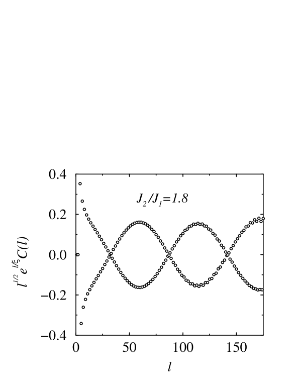
FIG. 9.: The correlation function $C(l)=\langle\vec{S}\cdot\vec{S}\rangle$, multiplied by $l^{1/2}e^{l/\xi}$, where the correlation length is $\xi=17.1$. The system size was $200\times 2$, and $m=350$ states were kept per block.

The correlation length $\xi$ was chosen to make the maximum in the “beat” amplitudes as constant as possible. The equal-time free boson propagator is:

$$\int{d\omega dk\over(2\pi)^{2}}{e^{ikl}\over\omega^{2}/v^{2}+k^{2}+\xi^{-2}}\propto\int dk{e^{ikl}\over\sqrt{k^{2}+\xi^{-2}}}\ \ {{}_{\longrightarrow}\atop{}^{l>>\xi}}\ \ l^{-1/2}e^{-l/\xi}.$$ (23)

The fit was also performed without the factor of $l^{1/2}$, with noticeably poorer results. Our results for the correlation length are subject to greater errors than, for example, the dimerization, both because a precise fitting function is not known and the errors in correlation functions are greater than in local measurements in DMRG calculations.

The resulting values for $\xi$ are shown in Figure 10. For comparison we show similar results for the ladder system shown in Fig. 2. The correlation length grows much more rapidly in the zigzag chain than in the ladder system. (These lengths correspond to considering the zigzag chain a $L\times 2$ system. If we consider it a single chain, these lengths would be multiplied by two.) Figure 11 shows the same results as a semilog plot. It appears that for the accessible values of $J_{2}/J_{1}$, the correlation length does not yet grow exponentially with $J_{2}/J_{1}$.

FIG. 10.: The correlation length as a function of $J_{2}/J_{1}$.

FIG. 11.: A semilog plot of the correlation length as a function of $J_{2}/J_{1}$.

FIG. 12.: The angle $\theta$ versus $J_{2}/J_{1}$.

By fitting $l^{1/2}e^{l/\xi}C(l)$ to a sinusoidal function with an arbitrary wavelength and phase, we were able to extract the incommensurate angle $\theta$, which is shown in Figure 12. In Figure 13, we plot $\theta-\pi/2$ versus $1/\xi$, for which we expect linear behavior near the origin. The solid line corresponds to

$$(2\xi)^{-1}=\frac{\theta}{\pi/2}-1.$$ (24)

Given the uncertainties in our procedures for extracting $\theta$ and $\xi$, our data points are reasonably consistent with this behavior.

FIG. 13.: $\theta-\pi/2$ versus $1/\xi$.

V Kondo Lattice

We consider a generalized one-dimensional Kondo lattice Hamiltonian:

$$H=\sum_{i}[-t(c^{\dagger}_{i}c_{i+1}+\hbox{h.c.})+J\vec{S}_{i}\cdot c^{\dagger}_{i}{\vec{\sigma}\over 2}c_{i}+K\vec{S}_{i}\cdot\vec{S}_{i+1}].$$ (25)

Here $c_{i,\sigma}$ anihilates an electron of spin $\sigma$ at site $i$ and $\vec{S}_{i}$ is a spin-1/2 operator. Sums over spin indices are implicit. We include an explicit nearest neighbour spin coupling, $K$. This (and longer range terms) would be generated by conduction electron exchange (the RKKY mechanism). It could also arise from other exchange mechanisms in some cases as for instance in the organic chain compound CuPC(I).[26, 27] We include it here because it allows for straightforward application of bosonization techniques.

In fact the limit to which our method applies is $J<<t,K$. In this limit, we are only concerned with the low energy degrees of freedom of the conduction electrons ($c_{i}$) and the spin chain. These can be represented in bosonized form, introducing spin ($\phi_{s1}$) and charge ($\phi_{c}$) bosons to represent the conduction electrons and an additional spin boson ($\phi_{s2}$) to represent the spin chain. This approach was attempted independently in Ref. [28] but we disagree with their conclusions as explained below. The two spins bosons turn out to be very similar to the ones discussed for two spin chains above. They spin bosons may equivalently be represented by the matrix fields $g_{i}$. For $J=0$, we obtain simply 3 decoupled free boson Hamiltonians (plus various irrelevant interactions involving $\phi_{s2}$). The velocities are $v_{F}=2t$ for $\phi_{c}$ and $\phi_{s1}$ and $v_{s}=\pi K/2$ for $\phi_{s2}$. We note that the theory is not Lorentz invariant due to the difference of velocities. To bosonize the Kondo interaction we need the bosonic representations for the conduction electron spin operator and the localized spin operators, $\vec{S}_{i}$. These are given by:

$$c^{\dagger}_{j}{\vec{\sigma}\over 2}c_{j} \approx (\vec{\rho}_{L1}+\vec{\rho}_{R1})+\hbox{constant}\cdot[e^{2ik_{F}j}\hbox{tr}(\vec{\sigma}g_{1})e^{i\sqrt{2\pi}\phi_{c}}+\hbox{h.c.}]$$ (26)

$$\vec{S}_{j} \approx (\vec{\rho}_{L2}+\vec{\rho}_{R2})+\hbox{constant}(-1)^{j}\hbox{tr}(\vec{\sigma}g_{2}).$$ (27)

Note that, away from half-filling, the continuum limit Hamiltonian only contains a marginal coupling of the currents:

$$H_{\hbox{int}u}=J(\vec{\rho}_{L1}+\vec{\rho}_{R1})\cdot(\vec{\rho}_{L2}+\vec{\rho}_{R2}).$$ (28)

At half-filling, the $2k_{F}$ oscillation becomes commensurate with the alternating localized spin operator and an additional relevant (dimension 3/2) term occurs:

$$H_{\hbox{int}a}=\lambda\hbox{tr}(\vec{\sigma}g_{1})\cdot\hbox{tr}(\vec{\sigma}g_{2})\cos(\sqrt{2\pi}\phi_{c}),$$ (29)

where $\lambda\propto J$.

The strong analogy with the two-chain spin system is now clear. The half-filled Kondo lattice resembles the standard spin ladder model, with a relevant inter-chain interaction. Away from half-filling the Kondo lattice is very closely analogous to the zigzag spin chain model. In this case there are no relevant charge interactions so we may expect a decoupled massless charge sector. The field theory describing the spin sector is identical to that occuring in the zigzag spin chain, except for the difference of spin-wave velocities for the two chains. In fact, this situation could also easily be realised in the zigzag spin chain by having different coupling constants $J_{2}$ and $J_{2}^{\prime}$ for the two chains. It is also clear that adding Hubbard interactions for the electrons does not change things very much, particularly away from half-filling. The charge excitations still decouple and remain gapless in that case. The scaling dimensions of various operators change with the Hubbard interaction strength, associated with rescaling the charge boson, in the standard way.

At half-filling we expect $H_{\hbox{int}a}$, which couples charge and spin modes, to produce a gap for all charge and spin excitations. The gaps should scale as $J^{2}$ for either sign of $J$. If we assume that the charge boson develops a gap and hence $<\cos(\sqrt{2\pi}\phi_{c})>\neq 0$, then the interaction in the spin sector reduces to the same one that occurs for the spin ladder, Eq. (11). As argued above, this should gap both spin excitations. A different conclusion was reached in Ref. [28], where it was claimed that $\phi_{+}$ does not appear in the interaction and hence remains massless. This incorrect conclusion was obtained because of a missing minus sign in the transformation from nonabelian to abelian bosons, Eq. (8). The neccessity for the minus sign in the lower left matrix element can be seen by observing that the constraint $\det g=1$ is not obeyed and $\hbox{tr}(\vec{\sigma}g)$ is not purely anti-hermitean, without it. (The “note added in proof” in Ref. [28] reflects a realization of this error.[29])

Away from half-filling, where the charge boson is massless, we may analyze the spin sector much as for the zigzag chain. In particular, the Kondo interaction renormalizes to zero in the ferromagnetic case, leaving all spin excitations gapless. In the antiferromagnetic case, we expect an exponentially small spin gap:

$$\Delta\propto e^{-\hbox{constant}(v_{F}+v_{s})/J}.$$ (30)

Fujimoto and Kawakami[28] assumed instead that J renormalized to some sort of strong coupling critical point corresponding to vanishing spin gap for 1 branch of spin excitations. This assumption seems rather unlikely from the point of view of the RG analysis, in light of the above comments, but was motivated by physical considerations. That is, it would seem that somehow the left-moving spin excitations from the localized spins interact with the right-moving spin excitations of the conduction electrons (and vice versa) to form a gap. While this seems reasonable at half-filling, it becomes difficult to understand away from half-filling. If we consider the strong Kondo coupling limit then localized spins form singlets with on-site conduction electrons. This clearly produces a gap at half-filling where there is one conduction electron for each localized spin. However, below half-filling there is an excess of localized spins which may produce gapless excitations. In fact, for the ordinary Kondo lattice model ($K=0$) at strong coupling, $J>>t$, it has been shown by Sigrist et al.[30] that these left over spins form a (gapless) ferromagnetic groundstate. At weaker coupling Sigrist et al. found a non-ferromagnetic phase whose properties were not very well characterized. Fujimoto et al.[28] assumed that this phase corresponded to a single species of gapless spin excitations (as well as gapless charge excitations).

We do not find this argument convincing and think that a spin-gap phase may occur at weak coupling. Evidence for this is provided by our analysis of the zigzag spin chain in the previous sections. Note that in that case also a transition to a gapless phase occurred for sufficiently large $J$, i.e. $J_{1}>J_{1c}\approx 4J_{2}$.

A related phase with a spin gap but no charge gap has been found numerically in the t-J model away from half-filling, at $J$ of order $t$. In this case, it is apparently not associated with any spontaneous discrete symmetry breaking, and may be thought of as a dimer fluid state.[31] The absence of spontaneous symmetry breaking is a consequence of the gapless charge excitations. The dimer order parameter also contains a charge factor which has vanishing expectation value when the charge gap vanishes.

There is actually a limit of the generalized Kondo lattice model, below half-filling, which is essentially equivalent to the t-J model:

$$J>>t,K>>t^{2}/J.$$ (31)

The large J condition forces all conduction electrons to form singlets with localized spins. The unpaired localized spins can effectively hop around via the hopping term. Their predominant interaction is the Heisenberg term, $K$. In addition they have various weak induced interactions[30] of $O(t^{2}/J)$. These are the interactions responsible for ferromagnetism in the pure Kondo lattice model at strong coupling. In the spin-gap phase of the t-J model these interactions cannot change the behavior provided that they are small enough compared to the gap. This essentially constitutes a proof (given the numerical results on the t-J model) that the generalized Kondo lattice model has a spin-gap phase somewhere in its phase diagram away from half-filling. How large a region of parameter space is in the spin-gap phase and whether it includes the pure Kondo lattice model for some range of doping and $J/t$ are open questions which we are investigating numerically.[32]

It was argued independently by Zachar et al. [33] that the Kondo lattice should have a spin gap away from half-filling using a different type of bosonization based on perturbing around a different limit of the model where the Kondo interaction is strongly anisotropic.

VI Conclusions

The zigzag spin chain is gapless for weak ferromagnetic interchain coupling, but has an exponentially small gap for small antiferromagnetic coupling. This phase has a weak spontaneous dimerization, or broken translational symmetry along with a finite-range incommensurate magnetic order.

Although we have presented results for a wide range of $J_{2}/J_{1}$, our primary focus has been on the large $J_{2}/J_{1}$ region, where the system is best thought of as two weakly coupled chains. Most previous work has focused on smaller values of $J_{2}/J_{1}$. Our results help to explain the behaviour of the quasi-one-dimensional antiferromagnet, SrCuO₂, studied in Ref. [2]. This compound is believed to be well described by the zigzag spin chain (with very weakly coupled pairs of chains) with $J_{2}\approx 1000K$ and $|J_{2}/J_{1}|$ in the range 10-1000. The susceptibility appears to go to a finite constant as $T\to 0$, apart from a low $T$ upturn attributed to impurities. This indicates the absence of a gap. This is to be expected from the results obtained here since the gap vanishes exponentially with $J_{2}/J_{1}$ and should be competely negligible for this range of couplings. Note that, if the interchain coupling had been of ladder type rather than zigzag type, this gap would have been much larger and perhaps observable in the available temperature range. We find that the gap is approximately $.42J^{\prime}$ where $J^{\prime}$ is the inter-chain coupling in the spin ladder, for $J^{\prime}<<J$. Thus the gap might have been as large as 40K in the spin-ladder case and could have shown up in the susceptibility measurements which went down to 1.7K.

The field theory description of the zigzag spin chain, in the limit, $J_{2}>>J_{1}$ is closely related to the field theory description of the decoupled spin sector in the doped generalized Kondo lattice in the limit $K,t>>J$. Our results on the zigzag spin chain suggest the existence of a spin-gapped phase in the doped Kondo lattice.

- [1] C.K. Majumdar and D.K. Ghosh, J. Math. Phys. 10, 1388 (1969).
- [2] M. Matsuda and K. Katsumata, J. Mag. Mag. Mat. 140-145, 1671 (1995).
- [3] E. Dagotto, J. Riera, and D.J. Scalapino, Phys. Rev. B45, 5744 (1992).
- [4] S.P. Strong, and A.J. Millis, Phys. Rev. Lett.69, 2419 (1992).
- [5] T. Barnes et al., Phys. Rev. B47, 3196 (1993).
- [6] T.M. Rice, S. Gopalan, and M. Sigrist, Europhys. Lett. 23, 445 (1993); M. Sigrist, T.M. Rice, and F.C. Zhang, Phys. Rev. B 49, 12058 (1994).
- [7] S.R. White, R.M. Noack, and D.J. Scalapino, Phys. Rev. Lett.73, 886 (1994).
- [8] H.J. Schulz, Phys. Rev. B53, 2959 (1996).
- [9] L. Balents and M.P.A. Fisher, UCSB preprint NSF-ITP-9523, cond-mat/9503045.
- [10] S.R. White, Phys. Rev. Lett.69, 2863 (1992), Phys. Rev. B48, 10345 (1993).
- [11] T. Tonegawa and I. Harada, J. Phys. Soc. Jpn. 56, 2153 (1987).
- [12] R.J. Bursill , G.A. Gehring, D.J.J. Farnell, J.B. Parkinson, Chen Zeng, T. Xiang, preprint, cond-mat/9511044.
- [13] R. Chitra, S. Pati, H.R. Krishnamurthy, D. Sen, and S. Ramasesha, Phys. Rev. B52, 6581 (1995).
- [14] R. Julien and F.D.M. Haldane, Bull. Am. Phys. Soc. 28, 34 (1983).
- [15] I. Affleck, Fields, Strings and Critical Phenomena, ed. E. Brézin and J. Zinn-Justin (North-Holland, Amsterdam, 1990), 563.
- [16] S. Eggert and I. Affleck, Phys. Rev. B46, 10866 (1992).
- [17] S. Eggert, preprint cond-mat/9602026.
- [18] K. Okamoto and K. Nomura, Physics Letters A 169, 433 (1992).
- [19] I. Affleck, T. Kennedy, E. Lieb and H. Tasaki, Comm. Math. Phys. 115, 477 (1988).
- [20] H.J. Schulz, Phys. Rev. B34, 6372 (1986).
- [21] S.P. Strong and A.J. Millis, Phys. Rev. Lett. 69, 2419 (1992).
- [22] D. G. Shelton, A. A. Nersesyan and A. M. Tsvelik, preprint, cond-mat/9508047.
- [23] R.M. Noack, S.R. White and D.J. Scalapino, in Computer Simulations in Condensed Matter Physics VII, Eds. D.P. Landau, K.K. Mon, and H.B. Schüttler (Springer Verlag, Heidelberg, Berlin, 1994), p. 85-98.
- [24] S.R. White, to be published.
- [25] E. Sorensen and I. Affleck, Phys. Rev. Lett. 71, 1633 (1993).
- [26] M.Y. Ogawa et al. Phys. Rev. Lett. 57, 1177 (1986); Phys. Rev. B39, 10682 (1989); J. Am. Chem. Soc 109, 1115 (1987).
- [27] G. Quirion et al. Phys. Rev. B37, 4272 (1988).
- [28] S. Fujimoto and N. Kawakami, J. Phys. Soc. Japan, 63, 4322 (1994).
- [29] N. Kawakami, private communication.
- [30] M Sigrist, H Tsunetsugu, K Ueda and TM Rice, Phys. Rev. B46, 13838 (1992).
- [31] M. Ogata, M. Luchini, S. Sorella and F. Assaad, Phys. Rev. Lett. 66, 2388 (1991); C. Hellberg and E. Mele, Phys. Rev. B48, 646 (1993).
- [32] A. Sikkema, S.R. White and I. Affleck, in progress.
- [33] O. Zachar, S.A. Kivelson and V.J. Emery, preprint, cond-mat/9508109.