Magnetic-field-enhanced outgoing excitonic resonance in multi-phonon Raman scattering from polar semiconductors

Abstract

A combined scattering mechanism involving the states of free electron-hole pairs (exciton continuum) and discrete excitons as intermediate states in the multi-phonon Raman scattering leads to (1) a strong increase of the scattering efficiency in the presence of a high magnetic field and to (2) an outgoing excitonic resonance: the two features are not compatible when only free pairs (leading to a strong increase of the scattering efficiency under the applied magnetic field) or discrete excitons (resulting in the outgoing resonance at the excitonic gap) are taken into account.

]

I Introduction

In a recent publication, we have shown that the strong outgoing resonance observed in high order multi-phonon resonant Raman scattering (MPRRS) from polar semiconductors can be explained when high energy intermediate electronic states belong to the excitonic continuum (approximated by free electron-hole pairs, EHP) and only couple to the bound excitonic state at the last stage of a scattering process. The high probability of decay into the continuum strongly opposes the MPRRS mechanism involving discrete excitons as the only intermediate states for explanation of the observed outgoing resonance at the ground excitonic transition (see Ref.  and references therein). Cooled by the emission of a sufficiently large number of LO-phonons, the EHP binds into an exciton whose energy is not enough for LO-phonon-assisted decay.

In this work we analyze the effects of a high magnetic field on the outgoing excitonic resonance considering, as in Ref. , the monomolecular creation of a cold exciton by the light-generated free EHPs which lose energy but preserve their spatial correlation through the interaction with LO-phonons.

II Model

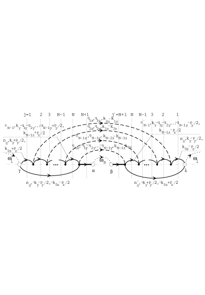
FIG. 1.: The diagram involving one discrete exciton intermediate state contributing to the MPRRS efficiency in the range of outgoing resonance. Hollow circles represent photon-electron-hole pair interaction, bold circles correspond to the electron-LO-phonon interaction while the square vertices are shown for discrete-continuum transitions. Solid lines above (below) the dash-dotted line represent the electrons (holes) and horizontal lines stay for bound excitons. Bold dashed lines connected left and right hand sides of the diagrams correspond to LO-phonons while the dotted lines represent incident (on the left and right sides) and scattered (in the center) photons.

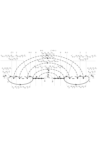
FIG. 2.: The diagram with two discrete exciton intermediate states contributing to the MPRRS efficiency in the range of outgoing resonance. The square vertices are shown for transitions between two states of discrete exciton and for discrete-continuum transitions.

The main contribution to the $N$-th order MPRRS efficiency follows from processes with one (Fig. 1) and two (Fig. 2) bound excitonic intermediate states at the last stage of the elementary scattering process. Only these contributions correspond to the cascade of transitions where the bound exciton cannot decay into the EHP continuum through the emission of LO-phonons. We assume $m_{h}>>m_{e}$ so that the hole energy is less than the energy of one LO-phonon and all phonons emitted by the EHP before its binding into a discrete exciton are emitted by the electron.

We use the Landau gauge ${\bf A}={\bf A}(0,xH,0)$ for a magnetic field directed along the $z$-axis and the corresponding wave functions of free EHPs. Only the ground state of the bound exciton is taken into account for discrete excitonic intermediate states in the last stage of the process. According to Refs. [3] and [4], the bound exciton wave function in a high magnetic field ($a>>a_{H}$, where $a$ is Bohr radius in a zero magnetic field and $a_{H}$ is the magnetic length, $a_{H}=\sqrt{\hbar c/eH}$) can be written as

$$\Psi^{exc}_{{\bf K}_{\perp}K_{z}}=\Psi_{\perp{\bf K}_{\perp}}\Psi_{\parallel K_{z}}~{},$$

where

$$\Psi_{\perp{\bf K}_{\perp}} = {\exp{\left[-\left|{\bf r}_{\perp}-{\bf r}_{\perp}({\bf K}_{\perp})\right|^{2}/(4a_{H}^{2})\right]}\over a_{H}\sqrt{2\pi L_{x}L_{y}}}$$ (1)

$$\times \exp\left\{i\left[(K_{x}-(y/a_{H}^{2}))R_{x}+K_{y}R_{y}\right.\right.$$ (2)

$$+ \left.\left.\Phi({\bf r}_{\perp},-{\bf K}_{\perp})+C(K_{x},K_{y})\right]\right\}~{},$$ (3)

and

$$\Phi({\bf r}_{\perp},-{\bf K}_{\perp}) = \left(xy/a_{H}^{2}-K_{x}x-K_{y}y\right)(m_{e}-m_{h})/2M~{},$$ (4)

$$C(K_{x},K_{y}) = a_{H}^{2}K_{x}K_{y}(m_{e}-m_{h})/2M~{},$$ (5)

$m_{e}$ $(m_{h})$ is the electron (hole) effective mass, $M=m_{e}+m_{h}$, ${\bf r}_{\perp}({\bf K}_{\perp})=(a_{H}^{2}/H)\left[{\bf H}\times{\bf K}_{\perp}\right]$ and ${\bf R}$, ${\bf r}$ are the center of mass and relative motion coordinates of an electron and hole. The longitudinal part $\Psi_{\parallel K_{z}}$ of the exciton wave function can be written as

$$\Psi_{\parallel K_{z}}={1\over\zeta\sqrt{a_{\parallel}L_{z}}}\exp(iK_{z}R_{z})\xi(z/a_{\parallel})~{},$$ (6)

where $\xi(s)$ describes the relative motion of the electron and hole along the magnetic field direction and satisfies the equation $\xi(s=0)=1.$ The constant $\zeta$ is determined by the normalization condition

$$\zeta^{2}=\int_{-\infty}^{\infty}ds~{}\xi^{2}(s)~{}.$$

We do not specify the exact form of $\xi(s)$ (see Ref. [3]) and introduce the two functions

$$\Theta(\alpha)=\int_{-\infty}^{+\infty}ds\exp{(i\alpha s)}\xi(s)$$

and

$$\eta(\alpha)=\int_{-\infty}^{+\infty}ds\exp{(i\alpha s)}\xi^{2}(s)$$

to be used below. For $\xi(s)=\exp{(-|s|)}$ one finds $\zeta=1$, $\eta(\alpha)=1/(1+\alpha^{2}/4)$ and $\Theta(\alpha)=2/(1+\alpha^{2})$. The wave function of Eq. (1) reduces to that of Ref. [3] when the Landau gauge is changed for the symmetric one.

III Scattering efficiency

The scattering efficiency can be written as[5]

$${d^{2}S\over d\Omega d\omega_{s}}={\omega_{s}^{3}\omega_{l}\over c^{4}}{n_{s}\over n_{l}}e_{s\alpha}^{\ast}e_{s\beta}e_{l\gamma}e_{l\lambda}^{\ast}S_{\alpha\gamma\beta\lambda}(\omega_{l},\omega_{s},{\bf\kappa}_{l},{\bf\kappa}_{s})~{},$$ (7)

where $S_{\alpha\gamma\beta\lambda}$ is the light scattering tensor of rank four, $c$ the light velocity in vacuum, $n_{l}$ $(n_{s})$, ${\bf e}_{l}$ $({\bf e}_{s})$, $\kappa_{l}$ $(\kappa_{s})$, $u_{l}$ $(u_{s})$ are the refractive index, polarization vector, wave vector, and group velocity of the incident (scattered) light, respectively. Using diagrammatic techniques, similar to those of Refs. , [4] and [6], we find for the contributions of the diagrams in Fig. 1 (Fig. 2)

$${d^{2}S_{Na(b)}\over d\Omega d\omega_{s}} = \sigma_{0}{\omega_{s}n_{s}\over\omega_{l}n_{l}}{|{\bf e}_{l}{\bf p}_{cv}|^{2}|{\bf e}_{s}{\bf p}_{cv}|^{2}\over\pi a_{H}^{2}m_{0}^{2}\hbar^{2}}$$ (8)

$$\times {\delta(\omega_{l}-\omega_{s}-N\omega_{LO})\over(\omega_{s}-\omega_{1H})^{2}+(\gamma_{excH}(0)/2)^{2}}{1\over L_{Na(b)}}~{},$$ (9)

where $\sigma_{0}=(e^{2}/m_{0}c^{2})^{2}$ and $\gamma_{excH}(0)$ is the inverse life time (broadening) of the exciton at the ground state with energy $E_{1H}=\hbar\omega_{1H}$. According to the assumption $m_{h}>>m_{e}$, the energy and the broadening of the hole have been neglected in all energy denominators. The quantity $L_{Na(b)}$ has dimensions of length and, for the diagram in Fig. 1

$${1\over L_{Na}}=\sum_{\beta}{D_{N\beta}\over\Lambda_{N\beta}Y_{N\beta}}\Xi_{n_{0},n_{N-1}}~{},$$ (10)

where the index $\beta$ designates the sequence of transitions made by the electron through Landau bands emitting successively $N-1$ phonons. It represents the set of $n_{0},n_{1},\dots,n_{N-1}$ Landau numbers and indices $i_{1},i_{2},\dots,i_{N-1}$. Each index $i$ may be $0$ or $1$: it is zero when the electron does not change the direction of motion along the magnetic field after the phonon emission and one when the sign of the velocity is opposite in the states before and after the phonon emission. In Eq. (10), $D_{N\beta}$ represents the integral

$$D_{N\beta} = {1\over K_{0}l}\int_{0}^{\infty}\prod_{j=1}^{N-1}\left[{dx_{j}\over K_{j}l}B_{n_{j-1}n_{j}}(x_{j})\chi^{i_{j}}(K_{j-1},K_{j},x_{j})\right]$$ (11)

$$\times \left\langle B_{n_{N-1}n_{0}}(x_{N})\chi^{i_{N}}(K_{N-1},K_{0},x_{N})\right\rangle~{},$$ (12)

where

$$K_{j} = \sqrt{2m_{e}\left(\omega_{l}-\omega_{gH}-n_{j}\omega_{eH}-j\omega_{LO}\right)/\hbar}~{},$$ (13)

$$l = \sqrt{\hbar/(2m_{e}\omega_{LO})}~{},$$ (14)

$$B_{nn^{\prime}}(x)={\min(n!,n^{\prime}!)\over\max(n!,n^{\prime}!)}e^{-x}x^{|n-n^{\prime}|}\left[L^{|n-n^{\prime}|}_{min(n,n^{\prime})}(x)\right]^{2}~{},$$ (15)

and

$$\chi^{i}(K,K^{\prime},x)=\left[x+a^{2}_{H}(K\mp K^{\prime})^{2}/2\right]^{-1}~{},$$ (16)

$\hbar\omega_{gH}=E_{g}+\hbar eH/(2\mu c)$, where $\mu=m_{e}m_{h}/M$ and $E_{g}$ is the gap. In Eq. (16), the $-~{}(+)$ sign corresponds to $i=0$ ($i=1$).

Note that $i_{N}=0$ when the direction of motion along magnetic field after emission of $N-1$ phonons coincides with an initial direction. In this case, $s=\sum_{n=1}^{N-1}i_{n}$ is an even number. For odd $s$ the direction of motion is opposite and $i_{N}=1$. The symbol $\langle\dots\rangle$ corresponds to the average over the directions of wavevectors ${\bf q}_{1\perp},{\bf q}_{2\perp},\ldots,{\bf q}_{N-1\perp}$ in the $xy$-plane, when $x_{j}=a_{H}^{2}q_{j\perp}^{2}/2$ and ${\bf q}_{N\perp}=-\sum_{i=1}^{N-1}{\bf q}_{i\perp}$. We used also

$$Y_{N\beta}=\prod_{j=0}^{N-1}(2\gamma_{j}/\alpha\omega_{LO})~{},~{}~{}\gamma_{j}=\gamma_{e}(n_{j},K_{j})~{},$$ (17)

where $\alpha$ is the Fröhlich coupling constant. When $\gamma_{e}(n,|k_{z}|)$ is determined by the interaction with LO-phonons, we find

$$\gamma_{e}(n,|k_{z}|) = \alpha\omega_{LO}\sum_{n^{\prime}}(2l|k_{z}^{\prime}|)^{-1}\int_{0}^{\infty}dxB_{nn^{\prime}}(x)$$ (18)

$$\times \left[\chi^{0}(|k_{z}|,|k_{z}^{\prime}|,x)+\chi^{1}(|k_{z}|,|k_{z}^{\prime}|,x)\right]~{},$$ (19)

$$k_{z}^{\prime} = \sqrt{k_{z}^{2}+2m_{e}\left[\omega_{eH}(n-n^{\prime})-\omega_{LO}\right]/\hbar}~{}~{}.$$ (20)

The sum over $n^{\prime}$ is limited by the condition that $k_{z}^{\prime}$ has to be real. When all $\gamma_{0},\gamma_{1},\ldots,\gamma_{N-1}$ are determined by the probability to emit an LO-phonon in a real transition, the substitution of Eq. (18) in Eq. (17) and multiplying the result by $l^{N}$ leads to $Y_{N\beta}$ defined in Eq. (134) of Ref. [6]. However, close to the resonance $\omega_{s}=\omega_{1H}$, the electron emitted $N-1$ LO-phonons occupies the state with the energy less than the energy of an LO-phonon. In this case $\gamma_{N-1}$ is determined by some other weaker scattering mechanism:

$$\gamma_{N-1}=\Gamma_{N-1}~{},~{}~{}~{}\Gamma_{N-1}\ll\gamma_{j}~{},~{}~{}~{}j=0,1,\ldots,N-2~{}~{}.$$ (21)

This leads to the result:

$$Y_{N\beta}=Y_{N-1\beta}{2\Gamma_{N-1}\over\alpha\omega_{LO}}~{}~{}.$$ (22)

The length $\Lambda_{N\beta}$ is defined as

$$\Lambda_{N\beta}=f_{N\beta}^{-1}(z=0)~{},~{}~{}~{}f_{N\beta}(z)=f^{i_{1}i_{2}\ldots i_{N-1}}(z)~{}.$$ (23)

For example, in the case $N=4$

$$f^{010}(z) = \left[f^{++--}(z)+f^{--++}(z)\right]/2~{}~{},$$ (24)

$$f^{++--}(z) = {1\over\lambda_{3}}\int_{-\infty}^{\infty}\left[\prod_{j=0}^{j=2}{dz_{j}\over\lambda_{j}}\right]\Upsilon^{+}\left({z_{0}\over\lambda_{0}}\right)\Upsilon^{+}\left({z_{1}-z_{0}\over\lambda_{1}}\right)$$ (25)

$$\times \Upsilon^{-}\left({z_{2}-z_{1}\over\lambda_{2}}\right)\Upsilon^{-}\left({z-z_{2}\over\lambda_{3}}\right)~{},$$ (26)

$$\Upsilon^{+}(t)=\left\{\begin{array}[]{cc}e^{-t},&t>0\quad;\\ 0,&t<0\quad,\end{array}\right.~{}~{}\Upsilon^{-}(t)=\left\{\begin{array}[]{cc}0,&t>0\quad;\\ e^{t},&t<0\quad,\end{array}\right.$$ (27)

$\lambda_{j}=\hbar K_{j}/m_{e}\gamma_{j}$ and $\gamma_{j}=\gamma_{e}(n_{j},K_{j})$.

In $p$-representation $f^{++--}(z)$ can be written as

$$~{}~{}~{}~{}f^{++--}(z)={1\over 2\pi}\int_{-\infty}^{\infty}dp\exp{(ipz)}$$ (28)

$$\left[(1+i\lambda_{0}p)(1+i\lambda_{1}p)(1-i\lambda_{2}p)(1-i\lambda_{3}p)\right]^{-1}~{}.$$ (29)

Finally, we have used the definition

$$\Xi_{n_{0},n_{N-1}} = {1\over\zeta^{4}}[\delta_{n_{0},0}\Theta^{2}(a_{\parallel}K_{0})+\delta_{n_{N-1},0}\Theta^{2}(a_{\parallel}K_{N-1})$$ (30)

$$- 2\delta_{n_{0},0}\delta_{n_{N-1},0}\Theta(a_{\parallel}K_{0})\Theta(a_{\parallel}K_{N-1})],$$ (31)

where $\Theta(\alpha)$ has been defined after Eq. (6).

We proceed to calculate the contribution of the diagram in Fig. 2. Since one of the intermediate states for the process of Fig. 2 corresponds to an exciton with ${\bf K}\not=0$, we need to comment on some details of the ground exciton dispersion $E_{exc}(K_{\perp},|K_{z}|)$. The energy $E_{exc}(K_{\perp},|K_{z}|)$ can be written as

$$E_{exc}(K_{\perp},|K_{z}|)=E_{gH}+E(K_{\perp})+\hbar^{2}K_{z}^{2}/(2M)~{}.$$ (32)

The function $E(K_{\perp})$ in some limits can be found in Ref. [3]. For our purposes it suffices to note that $E(K_{\perp}=0)=-\Delta E_{1H}$ is the exciton binding energy in a high magnetic field and $E_{1H}=E_{gH}-\Delta E_{1H}$. The contribution of the diagram in Fig. 2 is given by Eq. (8), where

$${1\over L_{Nb}} = \alpha\omega_{LO}{M\over m_{e}}\int_{0}^{x_{max}}dx\exp{(-x)}\sum_{\beta}{R_{N-1\beta}(x,K_{z0})\over\Lambda_{N-1\beta}Y_{N-1\beta}}$$ (33)

$$\times {[\eta(a_{\parallel}K_{z0}m_{h}/M)-\eta(a_{\parallel}K_{z0}m_{e}/M)]^{2}\over\zeta^{4}\left(x+a_{H}^{2}K_{z0}^{2}/2\right)^{2}lK_{z0}\gamma_{exc}(x,K_{z0})}~{}~{},$$ (34)

$K_{z0}=\sqrt{2M\left[\omega_{l}-\omega_{gH}-E(x)/\hbar-(N-1)\omega_{LO}\right]/\hbar}$ is the absolute value of the $z$-component of an exciton wave vector in the N-th real intermediate state, $x=a_{H}^{2}K_{\perp}^{2}/2$, and $\eta(\alpha)$ has been defined after Eq. (6). The $K_{\perp max}$ is a maximum value of $K_{\perp}$ allowed by energy conservation, i.e., under the condition that $K_{z0}$ is real. At variation of $K_{\perp}$ from zero to infinity the value $E(x)$ changes from $-\Delta E_{1H}$ to zero.[7] Therefore, in the range $\omega_{l}>\omega_{gH}+(N-1)\omega_{LO}$, we have $x_{max}\rightarrow\infty$, whereas for $\omega_{1H}+(N-1)\omega_{LO}<\omega_{l}<\omega_{gH}+(N-1)\omega_{LO}$ the values of $K_{\perp max}$ and $x_{max}$ are determined by the equation $\hbar\omega_{l}-E_{gH}-(N-1)\hbar\omega_{LO}=E(K_{\perp max})$. We used also the following definitions:

$$R_{N-1\beta}(K_{\perp},K_{z0})=$$ (36)

$${1\over lK_{0}}\int_{0}^{\infty}\prod_{j=1}^{N-2}\left[{dx_{j}\over lK_{j}}B_{n_{j-1}n_{j}}(x_{j})\chi^{i_{j}}(K_{j-1},K_{j},x_{j})\right]$$

$$\times \left\langle B_{n_{N-2}n_{0}}(x_{N-1})P_{\beta}(K_{\perp},K_{z0})\right\rangle~{}~{},$$ (37)

$$P_{\beta}(K_{\perp},K_{z0})=\left[\Upsilon_{\beta}(K_{\perp},K_{z0})+\Upsilon_{\beta}(K_{\perp},-K_{z0})\right]/2~{}~{},$$ (38)

and

$$\Upsilon_{\beta}(K_{\perp},K_{z0})={1\over\zeta^{4}}$$ (39)

$$\times \left\{x_{N-1}+(a_{H}^{2}/2)\left[(-1)^{p}K_{N-2}-K_{0}-K_{z0}\right]^{2}\right\}^{-1}$$ (40)

$$\times \left\{\delta_{n_{0},0}\Theta^{2}\left[a_{\parallel}\left(K_{0}+m_{h}K_{z0}/M\right)\right]\right.$$ (41)

$$+ \delta_{n_{N-2},0}\Theta^{2}\left[a_{\parallel}\left((-1)^{p}K_{N-2}+m_{e}K_{z0}/M\right)\right]$$ (42)

$$- 2\delta_{n_{0},0}\delta_{n_{N-2},0}\Theta\left[a_{\parallel}\left(K_{0}+{m_{h}\over M}K_{z0}\right)\right]$$ (43)

$$\times \left.\Theta\left[a_{\parallel}\left((-1)^{p}K_{N-2}-{m_{e}\over M}K_{z0}\right)\right]\right.$$ (44)

$$\times \left.\cos{\left[a_{H}^{2}\left({\bf q}_{N-1}\times{\bf K}_{\perp}\right)\right]}\right\}~{},$$ (45)

where $\beta$ is a set of indexes $n_{0},n_{1},\ldots,n_{N-2},i_{1},i_{2},\ldots,i_{N-2}$, $p=\sum_{n=1}^{N-2}i_{n}$. The variables of integration in Eq. (36) are $x_{j}=a_{H}^{2}q_{j\perp}^{2}/2$ with a constraint ${\bf q}_{N-1\perp}=-\sum_{i=1}^{N-2}{\bf q}_{i\perp}-{\bf K}_{\perp}$. The symbol $\langle\cdots\rangle$ denotes the average over angles which determine the direction of vectors ${\bf q}_{1\perp},{\bf q}_{2\perp},\ldots,{\bf q}_{N-2\perp},{\bf K}_{\perp}$ in the $xy$-plane.

IV Applicability limits

Let us discuss the applicability limits of the expressions for contributions of diagrams in Fig. 1 and Fig. 2. We assume that $\Delta E_{H}<\hbar\omega_{LO}$ and consider four intervals for the laser frequency:

$$(a)~{}~{}~{}~{}\omega_{1H}+(N-1)\omega_{LO}<\omega_{l}<\omega_{gH}+(N-1)\omega_{LO}~{},$$ (46)

$$(b)~{}~{}~{}~{}\omega_{gH}+(N-1)\omega_{LO}<\omega_{l}<\omega_{1H}+N\omega_{LO}~{},$$ (47)

$$(c)~{}~{}~{}~{}\omega_{1H}+N\omega_{LO}<\omega_{l}<\omega_{gH}+N\omega_{LO}~{},$$ (48)

$$(d)~{}~{}~{}~{}\omega_{l}>\omega_{gH}+N\omega_{LO}~{}.$$ (49)

The width of the intervals (a) and (c) is $\Delta E_{H}/\hbar$ and the one of interval (b) is $(\omega_{LO}-\Delta E_{H}/\hbar)$. The outgoing excitonic resonance coincides with the border of intervals (b) and (c).

Equations (8) and (10) for the contribution of the diagram in Fig. 1 are valid when $K_{N-1}$ is real for $n_{N-1}=0$ (see Eq. (13)). This is satisfied within the intervals (b), (c) and (d). In intervals (b) and (c), the value of $K_{N}(n_{N}=0)$ is pure imaginary and it is real in interval (d). This means that $\gamma_{N-1}$ is determined by Eq. (21) in (b) and (c) (therefore, in the vicinity of the outgoing resonance) and Eq. (22) is valid. Let us show that the $\Gamma_{N-1}$ cancels out of the expression for the contribution of the diagram in Fig. 1. To do this note that $\Lambda_{N\beta}$ from Eq. (23) is proportional to the mean free path

$${\cal L}_{N-1}={\hbar K_{N-1}\over m_{e}\Gamma_{N-1}}~{},$$ (50)

when ${\cal L}_{N-1}>>\lambda_{j},~{}j=0,1,\ldots,N-2$ . Thus,

$$\Lambda_{N\beta}^{-1}={\cal L}_{N-1}^{-1}T_{N\beta}~{}~{},$$ (51)

where $T_{N\beta}$ is a dimensionless function of $\lambda_{0},\lambda_{1},\ldots,\lambda_{N-2}$. For $N=2$ we find[4] that $(\Lambda_{20})^{-1}=f^{0}(z=0)=0$, $(\Lambda_{21})^{-1}=f^{1}(z=0)=1/(\lambda_{0}+\lambda_{1})$. This leads to $T_{20}=0$, $T_{21}=1$. Likewise, for $N=3$, $(\Lambda_{300})^{-1}=f^{00}(z=0)=0$, $(\Lambda_{310})^{-1}=f^{10}(z=0)=\lambda_{0}/((\lambda_{0}+\lambda_{1})(\lambda_{0}+\lambda_{2}))$, $(\Lambda_{311})^{-1}=f^{11}(z=0)=\lambda_{1}/((\lambda_{1}+\lambda_{0})(\lambda_{1}+\lambda_{2}))$, $(\Lambda_{301})^{-1}=f^{01}(z=0)=\lambda_{2}/((\lambda_{2}+\lambda_{0})(\lambda_{2}+\lambda_{1}))$. For $\lambda_{2}\rightarrow{\cal L}_{2}$ this lead to $T_{300}=0$, $T_{310}=\lambda_{0}/(\lambda_{0}+\lambda_{1})$, $T_{311}=\lambda_{1}/(\lambda_{0}+\lambda_{1})$ and $T_{301}=1$. Using Eqs. (22), (51) and (50) we obtain

$$(Y_{N\beta}\Lambda_{N\beta})^{-1}=(Y_{N-1\beta})^{-1}{\alpha\omega_{LO}m_{e}\over 2\hbar K_{N-1}}T_{N\beta}~{}~{},$$ (52)

Thus, the quantity $\Gamma_{N-1}$ does not appear in the final result.

Equations (8) and (33) for the contribution of Fig. 2 are valid when $K_{z0}$ is real which is true for all four frequency intervals. In (b), (c) and (d) the broadening $\gamma_{N-2}$ is determined by the probability to emit an LO-phonon, whereas $\gamma_{N-2}\rightarrow\Gamma_{N-2}$ in (a), where $\Gamma_{N-2}<<\gamma_{j}$, $j=0,1,\ldots,N-3$. Note that Eq. (33) does not content $\Gamma_{N-2}$ in the interval (a) as it was shown above. The contribution of Fig. 2 depends strongly on the behavior of $\gamma_{exc}(K_{\perp},K_{z0})$ in the denominator of Eq. (33). This is the inverse relaxation time of the exciton in the state with energy $E_{exc}(K_{\perp},K_{z0})=\hbar\omega_{l}-(N-1)\hbar\omega_{LO}$. For $E_{exc}(K_{\perp},K_{z0})>E_{1H}+\hbar\omega_{LO}$ the value of $\gamma_{exc}(K_{\perp},K_{z0})$ is determined by the probability to emit an LO-phonon and is proportional to $\alpha$. However, for $E_{exc}(K_{\perp},K_{z0})<E_{1H}+\hbar\omega_{LO}$, the real emission of one LO-phonon is impossible and $\gamma_{exc}(K_{\perp},K_{z0})$ is determined by other much weaker processes, so that $\gamma_{exc}(K_{\perp},K_{z0})\rightarrow\Gamma_{exc}(K_{\perp},K_{z0}),$ with $\Gamma_{exc}<<\gamma_{exc}$. The change of the scattering mechanism dominating the broadening takes place at the frequency corresponding to the outgoing excitonic resonance. Below this point, the contribution of Fig. 2 exceeds strongly the one of Fig. 1. Note that in this range we have to take into account other contributions involving processes with acoustic phonons (see below).

Finally, the pole approximation (i.e., real transitions) for integrals over $k_{0z},k_{1z},\ldots,k_{N-1z}$ for the contribution of Fig. 1 and over $k_{0z},k_{1z},\ldots,k_{N-2z}$ for Fig. 2 results in the constraints $N\geq 2$ and $N\geq 3$ for Eq. (10) and Eq. (33), respectively.

V Discussion and conclusions

Let us consider the resonant behavior of the MPRRS efficiency as a function of $H$ and $\omega_{l}$. We limit ourselves to the case $N\geq 3$ where both Eq. (10) and Eq. (33) are valid. Both contributions increase in the vicinity of $K_{0}=0$, which corresponds to $\omega_{lmax,m_{h}\rightarrow\infty}\simeq\omega_{gH}+n\omega_{eH}$. Taking into account the finite value of $m_{h}$ leads to an exact relation $\omega_{lmax}(n)=\omega_{gH}+eHn/\mu c$. This condition corresponds to the creation of EHPs in the vicinity of the Landau band bottoms. The resonant conditions can be achieved by changing either $H$ or $\omega_{l}$. The maxima in a magnetic field dependence take place at

$$H_{max}(n)={\mu c\over e}{\omega_{l}-\omega_{g}\over n+1/2}~{}~{},$$ (53)

being independent on the order $N$ of the scattering process. There is an additional resonance[4] for $N=3$ corresponding to the contribution of Fig. 2 at $\omega^{\prime}_{lmax,m_{h}\rightarrow\infty}\simeq\omega_{gH}+neH/m_{e}c+\omega_{LO}$. This resonance follows from the increase of $(\Lambda_{21})^{-1}=1/(\lambda_{0}+\lambda_{1})=1/(\hbar K_{0}/m_{e}\gamma_{0}+\hbar K_{1}/m_{e}\gamma_{1})$ in Eq. (33), when $K_{1}\rightarrow 0$, because of the divergence in $\gamma_{0}$ (see Eq. (18)). Note also that contribution of Fig. 2 is equal to zero[4] for $\omega_{lmin,m_{h}\rightarrow\infty}(n,N-1)=\omega_{gH}+neH/m_{e}c+(N-1)\omega_{LO}$.

Above the outgoing resonance the contributions of Fig. 1 and Fig. 2 in the MPRRS efficiency are of the same order of magnitude. However, as it was mentioned before, below the resonance the contribution of Fig. 2 strongly increases because of the strong increase in the exciton life time in the real intermediate state with the energy being too small for emission of an LO-phonon. In this range, other scattering processes like the absorption of LO-phonons, interaction with acoustic phonons, etc. have to be taken into account. We give now a qualitative picture of the process including into our consideration the distribution function of excitons with respect to $K_{\perp},~{}|K_{z}|$. Let us introduce the integral efficiency for the $N$-th order process as

$$S_{N}=\int\int{d^{2}S_{N}\over d\Omega d\omega_{s}}d\Omega d\omega_{s}={1\over u_{l}}\sum_{\bf\kappa_{s}}{\bar{W}_{sN}}~{},$$ (54)

where $u_{l}$ is the group velocity of incident light and ${\bar{W}_{sN}}$ the normalized probability to emit the scattered light quantum per unit time.[8] Equation (54) differs from Eq. (8) only by the absence of the factor $4\pi\delta(\omega_{l}-\omega_{s}-N\omega_{LO})$.

On the other hand,

$$\sum_{\bf\kappa_{s}}\bar{W}_{sN}=\sum_{K_{\perp},K_{z}}P_{excN-1}(K_{\perp},|K_{z}|)\gamma_{l}(K_{\perp},|K_{z}|)~{},$$ (55)

where $P_{excN-1}(K_{\perp},|K_{z}|)$ is the normalized dimensionless distribution function of excitons created by the light in a N-1 LO-phonon-assisted process and $\gamma_{l}(K_{\perp},|K_{z}|)$ the probability of an LO-phonon-assisted emission of the scattered light quantum which can be written as $\gamma_{l}(K_{\perp},|K_{z}|)=\sum_{\bf\kappa_{s}}w_{s}$ and

$$w_{s}={2\pi\over\hbar}\sum_{f}\left|\sum_{a}{\langle f|U_{s}|a\rangle\langle a|{\cal H}_{int}|i\rangle\over E_{i}-E_{a}+i\hbar\gamma_{a}/2}\right|^{2}\delta(E_{i}-E_{f})~{},$$ (56)

${\cal H}_{int}$ is Fröhlich interaction of the exciton with LO-phonons and $U_{s}$ represents the interaction of excitons with the light. The initial and final state energy is $E_{i}=E_{exc}(K_{\perp},|K_{z}|)$ and $E_{f}=\hbar\omega_{s}+\hbar\omega_{LO}$, respectively. The intermediate state energy $E_{a}=E_{aEHP}+\hbar\omega_{LO}$ includes both the discrete and continuum part of the excitonic dispersion. Let us separate $\gamma_{l}$ in two corresponding parts, $\gamma_{l}=\gamma_{ldisc}+\gamma_{lcont}$. The outgoing resonance is related to the contribution $\gamma_{ldisc0}$ to $\gamma_{ldisc}$ coming from the transition via ground state of the exciton. According to Eq. (56), we find

$$\gamma_{ldisc0}(K_{\perp},|K_{z}|)=4{n_{s}\omega_{s}\over\hbar c^{3}}\left({e\over m_{0}}\right)^{2}|{\bf e}_{s}{\bf p}_{cv}|^{2}$$ (57)

$$~{}~{}~{}~{}~{}~{}~{}{\alpha\omega_{LO}^{2}l\over K_{\perp}^{2}+K_{z}^{2}}{\exp{\left(-a_{H}^{2}K^{2}_{\perp}/2\right)}\over a_{\parallel}a_{H}^{2}\zeta^{6}}$$ (58)

$${[\eta(K_{z}a_{\parallel}m_{h}/M)-\eta(K_{z}a_{\parallel}m_{e}/M)]^{2}\over[\omega_{exc}(K_{\perp},|K_{z}|)-\omega_{1H}-\omega_{LO}]^{2}+\gamma^{2}_{excH}(0)/4}~{}.$$ (59)

Above the excitonic resonance, $\omega_{l}>\omega_{1H}+N\omega_{LO}$, we have

$$P_{excN-1}(K_{\perp},|K_{z}|)={W_{excN-1}(K_{\perp},|K_{z}|)\over\gamma_{exc}(K_{\perp},|K_{z}|)}~{}~{},$$ (60)

where $W_{excN-1}(K_{\perp},|K_{z}|)$ is the normalized number of excitons created per unit time in the volume $V_{0}$ in the $N-1$ LO-phonon-assisted process. The probability $W_{excN-1}(K_{\perp},|K_{z}|)$ has been calculated in Ref. [4] for $N=4$. Being used in Eq. (60) together with Eqs. (57), (54) and (55) it reproduces the result of Eqs. (8) and (33).

Note that above the outgoing resonance the distribution is not zero only in very narrow interval of energies[4] since $W_{excN-1}(K_{\perp},|K_{z}|)$ is proportional to $\delta[\omega_{l}-(N-1)\omega_{LO}-E_{exc}(K_{\perp},|K_{z}|)/\hbar]$. However, for $\omega_{l}$ below the resonance the distribution becomes smooth. If the most important mechanism in this range is the interaction with acoustic phonons, one has to take into account diagrams with external acoustic phonon lines. In the range (b) (see Eq. (46)) the smoothing of the distribution should be weaker than in the range (a). The reason of this is the kinetic energy of exciton in range (b) which is larger than the exciton binding energy. Since the probability of scattering and decay via the interaction with phonons are of the same order, the exciton decays after a few interactions with acoustic phonons. The decay of an exciton in the range (a) is suppressed because of its small energy. In this case, the distribution depends on the probability of non-radiative recombination. At zero magnetic field, the distribution of excitons in the range (a) has been considered in Refs. [9, 10, 11] and [12].

The smoothness of the distribution leads to $(i)$ the broadening of the MPRRS peaks in the range (b) and especially in the range (a) and to $(ii)$ the increase of the integral scattering intensity, since the diagrams with acoustic phonon lines give additional contributions into the MPRRS efficiency.

To summarize, we have shown that the outgoing excitonic resonance has to be strongly enhanced under a high magnetic field. Above the outgoing resonance, the scattering efficiency for $N\geq 3$ may be up to $\alpha^{-2}$ times stronger than in a zero magnetic field where the MPRRS efficiency is proportional to $\alpha^{3}$, whereas in a high magnetic field it is proportional to $\alpha$, as it follows from Eqs. (8), (10) and (33). The crossover from $\alpha^{3}$ to $\alpha$ results from the quasi-one-dimensional character of free EHPs in $N$ (Fig. 1) or $N-1$ (Fig. 2) intermediate states under a high magnetic field. The enhancement is also valid for the ranges (a) and (b) below the excitonic resonance, where one has to calculate the exciton distribution function taking into account the interaction with acoustic phonons. To the best of our knowledge such calculations have yet to be performed. However, the distribution function is proportional to the creation probability of excitons with energy in the interval between $0$ and $\hbar\omega_{LO}$ which is increased by $\alpha^{-2}$ times in a high magnetic field.[4] Thus, the MPRRS efficiency also increases below the excitonic resonance.

The integral efficiency as a function of $\omega_{l}$ has to be asymmetric with respect to the point $\hbar\omega_{l}=N\hbar\omega_{LO}+E_{1H}$ because of the strong increase in the exciton life time below the resonance and appearance of additional contributions from the processes with acoustic phonons.

REFERENCES

[1] on leave from the P. N. Lebedev Physical
Institute, Russian Academy of Sciences, Moscow, Russia
[2] V. I. Belitsky, A. Cantarero, S. T. Pavlov, M.
Cardona, A. V. Prokhorov, and I. G. Lang, Phys. Rev.
B 52, 11 920 (1995).
[3] L. P. Gor‘kov and I. E. Dzyaloshinsky,
Zh. Eksp. Teor. Fiz. 53, 717 (1967) [Sov. Phys. JETP 26, 449 (1968)].
[4] I. G. Lang, S. T. Pavlov and A. V. Prokhorov,
Zh. Eksp. Teor. Fiz. 106, 244 (1994) [Sov. Phys. JETP 79, 133 (1994)].
[5] S. T. Pavlov, Dr. Sci. Thesis, St. Petersburg State
University, St. Petersburg, 1979, p. 290; E. L. Ivchenko, I. G.
Lang, and S. T. Pavlov, Fiz. Tverd. Tela (St. Petersburg) 19, 1751 (1977) [Sov. Phys. Solid State 19, 718 (1977)];
E. L. Ivchenko, I. G. Lang, and S. T. Pavlov, Phys. Stat. Solidi
b 85, 81 (1978).
[6] V. I. Belitsky, M. Cardona, I. G. Lang and
S. T. Pavlov,
Phys. Rev. B 46, 15767 (1992).
[7] For there is
no bound exciton in a high magnetic field ().
However, in the integral of Eq. (33) only the
range is important, a fact which allows us to integrate in the
interval between zero and infinity.
[8] I. G. Lang, S. T. Pavlov, A. V. Prokaznikov and
A. V. Goltsev, Phys. Stat. Solidi b 127, 187 (1985).
[9] E. F. Gross, S. A. Permogorov and V. V. Travnikov,
J. Phys. Chem. Sol. 31, 2595 (1970).
[10] R. Planel, A. Bonnot and C. Benoit a la Guillaume,
Phys. Stat. Solidi b 58, 251 (1973).
[11] C. Trallero Giner, O. Sotolongo Costa,
I. G. Lang, and S. T. Pavlov,
Fiz. Tverd. Tela (St. Petersburg) 28, 2075 (1986) [Sov.
Phys. Solid State 28, 1160 (1986)].
[12] C. Trallero Giner, O. Sotolongo Costa,
I. G. Lang, and S. T. Pavlov,
Fiz. Tverd. Tela (St. Petersburg) 28, 3152 (1986) [Sov.
Phys. Solid State 28, 1774 (1986)].