SIMULATIONS OF DENSE GRANULAR FLOW:
DYNAMIC ARCHES AND SPIN ORGANIZATION

Abstract

We present a numerical model for a two dimensional (2D) granular assembly, falling in a rectangular container when the bottom is removed. We observe the occurrence of cracks splitting the initial pile into pieces, like in experiments. We study in detail various mechanisms connected to the ‘discontinuous decompaction’ of this granular material. In particular, we focus on the history of one single long range crack, from its origin at one side wall, until it breaks the assembly into two pieces. This event is correlated to an increase in the number of collisions, i.e. strong pressure, and to a momentum wave originated by one particle. Eventually, strong friction reduces the falling velocity such that the crack may open below the slow, high pressure ‘dynamic arch’. Furthermore, we report the presence of large, organized structures of the particles’ angular velocities in the dense parts of the granulate when the number of collisions is large.
PACS: 46.10.+z, 05.60+w, 47.20.-k

I Introduction

The flow behavior of granular media in hoppers, pipes or chutes has received increasing interest during the last years. For a review concerning the physics of granular materials, see [1, 2] and refs. therein.

The complete dynamical description of gravity driven flows is an open problem and for geometries like hoppers or vertical pipes, several basic phenomena, are still unexplained. In hoppers intermittent clogging due to vault effects [3], density waves in the bulk [4] or 1/$f$ noise of the outlet pressure, have been reported from experiments [5]. In a vertical pipe geometry, numerical simulations on model systems with periodic boundary conditions [6, 7] and also analytical studies [8] show density waves. But so far, experimental evidence of density waves is only found in situations where pneumatic effects, i.e. gas-particle interactions, are important [9].

In the rapid flow regime, kinetic theories [10, 11] describe the behavior of the system introducing the granular temperature as a measure of the velocity fluctuations. In quasistatic situations, also arching effects and particle geometry get to be important. Under those conditions, kinetic theories and also continuum soil mechanics do not completely describe all the phenomena observed. The complicated particle-wall and particle-particle interactions [12, 13, 14], possible formation of stress chains in the granulate and also stress fluctuations [15, 16] undoubtedly require further experimental, theoretical and simulation work.

Following recent research on model granular systems [15, 16, 17, 18, 19, 20, 21] we focus here on the problem of a 2D pile made up of rather large spheres enclosed in a rectangular container with transparent front and back walls, separated by slightly more than one particle diameter. Recent observations of approximately V-shaped microcracks in vertically vibrated sand-piles [17] were complemented by recent experiments and simulations of the discontinuous decompaction of a falling sandpile [22]. From experiments Duran et al. [22] find the following basic features: In a system with polished laterals walls, cracks are unlikely to appear during the fall, i.e. the pile will accelerate continuously, with an acceleration value depending on the aspect ratio of the pile and on the friction with the walls. In a system with rather poorly polished walls (a surface roughness of more than 1 $\mu$m in size), cracks occur frequently. A crack in the lower part of the pile grows, whereas a crack in the upper part is unstable and will eventually close. These experimental findings can be understood from a continuum approach based on a dynamical adaptation of Janssen’s model [3, 22]. Nevertheless, not all of the discontinuous phenomena, such as the reasons for the cracks, can be explained by such a continuum model. In previous works, numerical simulations were used to parallel the experiments and to analyze the falling pile for different material’s parameters [22, 23]. Though the simulations are dynamic, in contrast to an experiment which starts from a static situation, a reasonable phenomenological agreement was found. Furthermore, simulations were able to correlate the existence of long range cracks to strong local pressure on the walls. The increase in pressure was found to be about one order of magnitude [22]. In this work we use the numerical model of Refs. [24, 22, 23, 25] and investigate in detail how a crack occurs. In particular, we follow one specific crack and try to extract the generic features that could be relevant for a more involved theoretical description of the behavior of granular materials.

We briefly discuss the simulation method in section II and present our results in section III which consists of three main parts: Firstly, we present stick-slip behavior and a local organization of the spins in subsection III A. Secondly, we describe in how far the number of collisions, the kinetic energy and the pressure are connected in III B and finally we present long range organization and momentum waves in subsection III C. We summarize and conclude in section IV.

II The Simulation Method

Our simulation model is an event driven (ED) method [24, 22, 25, 26, 27, 28] based upon the following considerations: Particles undergo a parabolic flight in the gravitational field until an event occurs. An event may be the collision of two particles or the collision of one particle with a wall. Particles are hard spheres and interact instantaneously; dissipation and friction are only active on contact. Thus we calculate the momentum change using a model that is consistent with experimental measurements [28]. From the change of momentum we compute the particles’ velocities after a contact from the velocities just before contact. We account for energy loss in normal direction, as for example permanent deformations, introducing the coefficient of normal restitution, $\epsilon$. The roughness of surfaces and the connected energy dissipation, is described by the coefficient of friction, $\mu$, and the coefficient of maximum tangential restitution $\beta_{0}$. For interactions between particles and walls we use an index $w$, e.g. $\mu_{w}$. Due to the instantaneous contacts, i.e. the zero contact time, one may observe the so-called ‘inelastic collapse’ in the case of strong dissipation. For a discussion of this effect see McNamara and Young [29] and refs. therein. Despite this problem, we use the hard sphere ED simulations as one possible approach, since also the widely used soft sphere molecular dynamics (MD) simulations may lead to complications like the ‘detachment-effect’ [30, 31, 32] or the so-called ‘brake-failure’ for rapid flow along rough walls [33]. Recent simulations of the model system, described in this study, using an alternative simulation method, the so called ’contact dynamics’ (CD) [14], also lead to cracks [34]. The CD method has a fixed time-step, in contrast to ED where the time-step is determined by the time of the next event.

From the momentum conservation laws in linear and angular direction, from energy conservation, and from Coulomb’s law we get the change of linear momentum of particle 1 as a function of $\epsilon$, $\mu$, and $\beta_{0}$ [25]:

$$\Delta\vec{P}=-m_{12}(1+\epsilon)\vec{v}_{c}^{(n)}-{\frac{2}{7}}m_{12}(1+\beta)\vec{v}_{c}^{(t)},$$ (1)

with the reduced mass $m_{12}=m_{1}m_{2}/(m_{1}+m_{2})$. For particle-wall interaction, we set $m_{2}=\infty$ such that $m_{12}=m_{1}$. (n) and (t) indicate the normal and tangential components of the relative velocity of the contact points

$$\vec{v}_{c}=\vec{v}_{1}-\vec{v}_{2}-\left({{\frac{d_{1}}{2}}\vec{\omega}_{1}+{\frac{d_{2}}{2}}\vec{\omega}_{2}}\right)\times\vec{n},$$ (2)

with $\vec{v}_{i}$ and $\vec{\omega}_{i}$ being the linear and angular velocities of particle $i$ just before collision. $d_{i}$ is the diameter of particle $i$ and the unit vector in normal direction is here definded as $\vec{n}=(\vec{r}_{1}-\vec{r}_{2})/|\vec{r}_{1}-\vec{r}_{2}|$. Paralleling $\epsilon$, the (constant) coefficient of normal restitution we have $\beta$, the coefficient of tangential restitution

$$\beta=\min\left[\beta_{0},\beta_{1}\right].$$ (3)

$\beta_{0}$ is the coefficient of maximum tangential restitution, $-1\leq\beta_{0}\leq 1$, and accounts for energy conservation and for the elasticity of the material [28]. $\beta_{1}$ is determined using Coulomb’s law such that for solid spheres $\beta_{1}=-1-(7/2)\mu(1+\epsilon)\cot\gamma$ with the collision angle $\pi/2<\gamma\leq\pi$ [25]. Here, we simplifed the tangential contacts in the sense that exclusively Coulomb-type interactions, i.e. $\Delta P^{(t)}$ is limited by $\mu\Delta P^{(n)}$, or sticking contacts with the maximum tangential resitution $\beta_{0}$ are allowed. Sticking corresponds thus to the case of low tangential velocity whilst the Coulomb case corresponds to sliding, i.e. a comparatively large tangential velocity. For a detailed discussion of the interaction model used see Refs. [24, 25, 28].

III Results

Since we are interested in the falling motion of a compact array of particles, we first prepare a convenient initial condition. Here, we use $N=1562$ particles of diameter $d=1$ mm in a box of width $L=20.2d$, and let them relax for a time $t_{r}$ under elastic and smooth conditions until the density and energy profiles do not change any longer. The choice of $L$ is quite arbitrary, however, we wanted to start with a triangular lattice with a lattice constant of $d(1+\Delta)$ and $\Delta$ to be small but larger than zero, i.e. $\Delta=0.01$. We tested several height to width ratios $S=H/L$ of the system and found e.g. the same behavior as in experiments, i.e. the larger $S$, the stronger are the effects discussed in the following. The average velocity of the resulting initial condition is $\overline{v}=\sqrt{<v^{2}>}\approx 0.05$m/s.

[]

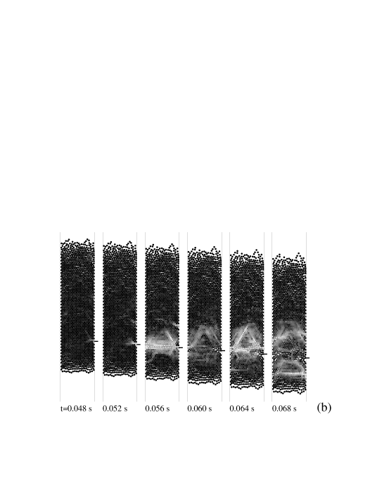
FIG. 1.: (a) Snapshots of a typical experiment (left) and a simulation (right) with $N$ =1562 particles, at time $t$ = 0.06 s, in a pipe of width $L/d$ = 20.2. We used here $\epsilon$ = 0.96, $\epsilon_{w}$ = 0.92, $\mu$ = 0.5, $\mu_{w}$ = 1.0, and $\beta_{0}=\beta_{0w}$ = 0.2. (b) Snapshots from a simulation with almost the same parameters as in (a), but here $\epsilon$ = 0.90, $\epsilon_{w}$ = 0.90, and $\mu_{w}$ = 0.5. The greyscale indicates the number of collisions per particle per millisecond. Black and white correspond to no collision or more than ten collisions respectively. (c) Here only the selected particles #369, #370, #371, #390, #409, and #428 from (b) are plotted to illustrate their motion. The vertical line indicates the right wall.

The kinetic energy connected to $\overline{v}$ is comparable to the potential energy connected to the size of one particle. Due to this rather low kinetic energy, the array of particles is arranged in triangular order, except for a few layers at the top. Some tests with different values of $\overline{v}$ lead to similar results as long as $\overline{v}$ is not too large. The larger $\overline{v}$, the more particles belong to the fluidized part of the system at the top and in the fluidized part of the system we can not observe cracks. For lower values of $\overline{v}$ we observed an increasing number of events per unit time and thus increasing computational costs for the simulation. At $t=0$ we remove the bottom, switch on dissipation and friction and let the array fall.

Performing simulations with different initial conditions and different sets of material’s parameters, we observe strong fluctuations in position and shape of the cracks. However, the intensity or the probability of the cracks seems to depend on the material’s parameters rather than on the initial conditions. The behavior of the system depends on friction and on dissipation as well: For weak friction we observe only random cracks, which would occur even in a dense hard sphere gas without any friction, simply due to random fluctuations and the internal pressure. With increasing friction, cracks may even span the whole system and sometimes be correlated to slip planes. Furthermore, we observe cracks to occur more frequent for lower dissipation.

In Fig. 1(a) we present typical snapshots of an experiment and of a simulation at time $t$ = 0.04 s. We observe long range cracks from both, experiments and simulations as well. For the experiment we use a container of width $L/d$ = 24 with 103 layers of oxidized aluminum particles. The vertical 2D cell is made up of two glass windows for visualisation and of two lateral walls made of plexiglass. The gap between the glass windows is a little larger than the bead diameter, what leads to a small friction between particles and front/back walls, while the friction with the side walls may be large. Different heights and wall-materials were used and the results could be scaled with a characteristic length $\xi=L/(2K\mu_{w})$, with the dimensionless parameter $K$ which characterizes the conversion of vertical to tangential stresses and the coefficient of friction $\mu_{w}$. The scaling in the regime before cracks occur leads to the value $K\mu_{w}\approx 0.12$. For a more detailed description of the experimental setup and data see Ref. [22]. In the simulation of Fig. 1 we have $N$ = 1562 and the parameters $L/d$ = 20.2, $\epsilon$ = 0.96, $\epsilon_{w}$ = 0.92, $\mu$ = 0.5, $\mu_{w}$ = 1.0, and $\beta_{0}=\beta_{0w}$ = 0.2. We varied the coefficients of friction in the intervals $0\leq\mu\leq 1$ and $0\leq\mu_{w}\leq 10$. Furthermore, we varied the coefficients of restitution in the range $0.80\leq\epsilon or\epsilon_{p}\leq 0.98$. However, the occurrence of cracks is quite independent of the parameters used, as long as the coefficients of friction, $\mu$ and $\mu_{w}$ are sufficiently large. Furthermore, cracks occur faster for stronger dissipation since a highly dissipative block dissipates the initial energy faster.

For the above parameters, we find - like in experiments - a large number of cracks, overlapping and interferring. In the upper part of both, experiment and simulation, we sometimes observe cracks only on one side. In contrast to Fig. 1(a) we present in Fig. 1 (b) a specific simulation with only one strong crack, on which we focus in more detail. This crack separates the system into a large upper and a small lower part and is best visible in Fig. 1(b) at $t$ = 0.068 s. Here we use a reduced wall friction, i.e. $\mu_{w}$ = $\mu$ = 0.5, and stronger dissipation, i.e. $\epsilon_{w}=\epsilon=0.9$, while all other parameters, including the initial configuration, are the same as for (a).

In order to distinguish consistently, we will refer to the simulation with large $\mu_{w}$ as simulation (a), and to the simulation with small $\mu_{w}$ as simulation (b) in the following.

The important feature of the crack in Fig. 1(b) is that it seems to be connected to one single particle. We indicate the vertical position of particle #371 with a small bar in Fig. 1(b). The crack of simulation (b) is connected to an increase of the number of collisions per particle, indicated by the greyscale on Fig. 1(b). Black or white correspond to zero or more than twenty collisions during the last millisecond respectively. Note that the increase in the number of collisions is here equivalent to an increase in pressure. Already at time $t$ = 0.048 s, particle #371 peforms more collisions than the average particle. The pressure around particle #371 increases and at $t$ = 0.056 s a region in which the particles perform a large number of collisions spans the whole width of the container. We call such an array of particles under high pressure ‘dynamic arch’. At $t$ = 0.060 s the pressure decreases and a large crack opens below particle #371. At later times, we observe new pressure fluctuations in the array. In conclusion, a crack seems to begin at one point, i.e. one particle, where the pressure increases accidentally.

Before we look in more detail at the behavior of particle #371, we present for convenience, a picture of some selected particles around #371 from (b), in Fig. 1(c).

A Evidence for Stick-Slip Behavior

From Fig. 1(b) we evidenced that a crack may originate from one particle only. Now we are interested in the velocity of one specific particle during its fall. Following the order of simulations (a) and (b) we firstly present the case of large wall friction (a) and secondly the case of smaller wall friction (b) in the following. Remember that particle #371 is the origin of one single crack in simulation (b), while its behavior is similar to the behavior of many others, close to the boundary, in simulation (a).

FIG. 2.: Plot of the angular velocity, $\omega r$, and of the linear, vertical velocity, $V_{z}$, of particle #371 versus time. The simulations are the same as in Fig. 1(a) and (b). The line $-gt$ corresponds to a freely falling particle.

Due to gravity, the particle is accelerated downwards and after a collision with the right wall it will presumably rotate counterclockwise. Therefore, we compare the linear velocity, $V_{z}$, with the rotational velocity of the surface, $\omega r$. In Fig. 2 we plot both, the linear vertical and the angular velocity of particle #371 as a function of time. The horizontal line indicates zero velocity and the diagonal line indicates the free fall velocity, $-gt$. The full curve gives the (negative) linear velocity in vertical direction, $V_{z}$, while the rotational velocity of the surface, $\omega r$, is given by the dashed curve. Negative $\omega r$ values correspond to counterclockwise rotation and for $V_{z}=\omega r$ we have the contact point of the particle at rest relative to the wall. The particle adapts rotational and linear velocity, or in other words, the contact point sticks. This event occurs when the two curves merge. In Fig. 2(a) we observe a small angular velocity up to $t\approx$ 0.02 s when particle #371 first sticks. Note that in this simulation (a) #371 can not be identified as the initiator of one of the numerous cracks; however, it sticks and slips several times. An increase in angular velocity goes ahead with a decrease of linear velocity due to momentum conservation. At larger times we observe the angular velocity decreasing, i.e. the particle slips, and short time after, sticks again.

FIG. 3.: Plot of the angular velocities of the particles #371, #390, #409, and #428 for the same simulations as in Fig. 1(a) and (b). These particles were initially arranged on a line, tilted clockwise by 60 degrees from the horizontal, see Fig. 1(c).

Now we focus on simulation (b) and the behavior of the particle, from which the crack started. In Fig. 2(b) we observe a small angular velocity up to $t\approx$ 0.050 s. At $t$ = 0.055 s the velocities are adapted for some 0.005 s before the particle slips again. Since the pressure fluctuations are visible in Fig 1(b) already at $t$ = 0.048 s, we conclude that pressure fluctuations in the bulk lead to a sticking of a particle surface on the wall. This particle is slowed down and thus will perform more collisions with those particles coming from above, what leads to an increase of pressure. An increase of pressure allows, in general, a strong Coulomb friction and thus a sticking of the contact point. When pressure decreases, the particle surface does not longer stick on the wall.

Since the sticking might also occur between particles, we examine the angular velocity of the particles in the neighborhood of the sticking particle, i.e. the particles to the upper left of particle #371. In Fig. 3 we plot the angular velocities of particles #371, #390, #409, and #428 for the simulations (a) and (b). We observe from both figures as a response to friction, an auto-organization of the spins as also observed in 1D experiments and simulations of rotating frictional cylinders [12, 13]. Spin stands here for the direction of angular velocity of a particle. We see that the direct neighbor of #371 to the left and upwards, i.e. #390, rotates in the opposite direction as #371. Thus a counterclockwise rotation of particle #371 leads to a clockwise rotation of #390. This is consistent with the idea of friction reducing the relative surface velocity. The next particle to the upper left, i.e. #409, is again rotating couterclockwise, following the same idea of frictional coupling. In Fig. 3(a) we observe only a weak coupling between #409 and #428, whereas in Fig. 3(b) particle #428 is also rotating clockwise, even when the absolute value of the angular velocity is smaller. Thus we have not only a stick-slip behavior of particles close to the side walls, but also a coupling of the spins of neighboring particles. If the coupling is strong enough, we observe an alternating, but decreasing angular velocity along a line. We will return to this observation in subsection III C.

B Number of Collisions, Kinetic Energy and Pressure

Since the occurrence of a crack is, in general, connected to a large number of collisions, we plot in Fig. 4 the number of collisions per particle per millisecond, $N_{c}$, for simulations (a) and (b). In Fig. 4(a) we observe an increase in the number of collisions, which is related to the first sticking event of particle #371. However, particles deep in the array possibly perform much more collisions, see #428 in Fig. 4(a). Obviously, an increase in $N_{c}$ for one particle is connected to an increase in $N_{c}$ for the neighbors. In Fig. 4(b) we find values of $N_{c}$ comparable for direct neighbors, i.e. #371 and #390. At $t$ = 0.056 s we observe a drastic increase in $N_{c}$ which also involves the particles deeper in the array, i.e. #409 and #428.

FIG. 4.: Log-lin plot of the number of collisions, $N_{c}$, per millisecond (ms) as a function of simulation time, $t$. Plotted is $N_{c}$ for the four particles noted in the figure. The data are from the same simulations as already presented in Fig. 1 (a) and (b).

In order to illustrate the reduced falling velocity, connected to a large number of collisions we plot in Fig. 5 the averaged kinetic energy $K$ for particles between heights $z$ and $z+dz$ (we use here $dz$ = 0.002 m). We plot $K=(1/N)\Sigma_{i=1}^{N}v_{i}^{2}$ (disregarding the mass of the particles), as a function of the height, $z$. Note that $v_{i}$ is the velocity of one particle relative to the walls, and not relative to the center of mass of the falling sandpile. We observe different behavior for the simulations (a) and (b): A rather homogeneous deceleration of the pile in (a) and one ’dynamic arch’ connected to a strong deceleration in (b). For strong friction at the walls (a), all particles in the system are slowed down due to frequent collisions of the particles with the side walls and inside the bulk. For the times $t$ = 0.05, 0.06, and 0.08 s we observe, from the bottom indicated by the left vertical line in Fig. 5, a decreasing $K$ with increasing height $z$ up to $z\approx 0.02$ m, where the slope of $K$ almost vanishes. In Fig. 5(b) the particles are falling faster at the beginning until the first dynamic arch occurs at $t\approx 0.056$ s, see Fig. 1(b). The high pressure exerted on the walls, together with the tangential friction at the walls, leads to a local deceleration, i.e. the dip in the $K$ profile for $t$ = 0.06 s. This dip identifies a dynamic arch of slow material which temporarily blocks the flow. Later in time, the particles from above arrive at the slower dynamic arch, which again leads to great pressure, a large number of collisions and thus to a further reduction of $K$ (see the $K$ profile for $t$ = 0.08 s).

FIG. 5.: Plot of the kinetic energy $K$ as a function of height $z$ for different times for the same simulations as already presented in Fig. 1 (a) and (b).

In order to understand how the pressure in the bulk is connected to $N_{c}$ and $K$ we plot in Fig. 6 the particle-particle pressure, $pp$, in arbitrary units as a function of height for the simulations (a) and (b). $pp$ is here defined as the sum over the absolute normal part of momentum change

$$pp(z,t)=\Sigma|\Delta\vec{P}^{(n)}|,$$ (4)

for each particle in a layer $[z,z+dz]$ in a time interval $[t,t-dt]$. For this plot we use $dz=\sqrt{3}d$ (what corresponds to a height of two particle layers) and the integration time is here $dt$ = 0.005 s. For strong wall friction and low dissipation (a), we observe already at $t$ = 0.02 s a quite strong pressure with a maximum close to the bottom of the pile. At $t$ = 0.05 s the maximum in pressure moved upwards, not only within the falling pile but also in coordinate $z$. Furthermore, the maximum is about one order of magnitude larger than before. Later, the pressure peak moved further upwards and at $t$ = 0.06 s begins to decrease until at larger times the array is dilute and pressure almost vanished. For weak wall friction (b) we find only a weak pressure at time $t$ = 0.02 s until at time $t$ = 0.06 s a sudden increase of pressure, connected to the increase in $N_{c}$ and the decrease in $K$, appears. The occurrence of two pressure peaks of different amplitude (small pressure at the bottom and large pressure at the top) is consistent with the predictions of Duran et al. [22], which state that a small lower pile will be decelerated less than a large upper pile. Thus the crack continues opening.

FIG. 6.: Log-lin plot of the pressure, $pp$, as a function of height $z$ for different times for the same simulations as already presented in Fig. 1 (a) and (b).

C Long Range Rotational Order and Momentum Waves

We have learned from Figs. 2 and 3 that, connected to a large number of collisions, the direction of the angular velocity, i.e. the spin of the particles, may be locally arranged in an alternating order along lines of large pressure. In order to proof that this is not only a random event we plot in Fig. 7(a) some snapshots from simulation (a) and indicate clockwise and counterclockwise rotation with black and white circles respectively. We observe, at least in some parts of the system, that spins of the same direction are arranged along lines. The spins of two neighboring lines have different directions. The elongation of the ordered regions may be comparable to the size of the system. Note, that lines of equal spin are perpendicular to a line of strong pressure, such that the order in Fig. 7(a) indicates an arch like structure.

In Fig. 7(b) we plot snapshots from simulation (b) and plot the change of velocity, i.e. $\Delta v_{x}=v_{x}(t+\delta t)-v_{x}(t)$ and $\Delta v_{z}=v_{z}(t+\delta t)-v_{z}(t)+g~{}\delta t$ with $\delta t=10^{-3}$ s. Comparing Figs. 1(b) and 7(b) we identify the large number of collisions, starting from particle #371, with a momentum wave propagating from #371 towards the left wall and also diagonally upwards. When the momentum wave arrives at the left wall it is reflected and moves mainly upwards. We relate this to the fact that the material below the dynamic arch is falling faster than the dynamic arch, such that not much momentum change takes place downwards. After several milliseconds the momentum wave is not longer limited to some particles only, but has spread and builds now an active region with great pressure, i.e. the dynamic arch.

[]

FIG. 7.: (a) Snapshots of the simulation from Fig. 1(a) at different times. The greyscale indicates here the direction of the angular velocity, i.e. black and grey correspond to clockwise and counterclockwise rotation respectively. (b) Snapshots from the simulation from Fig. 1(b) at different times. The lines indicate for each particle the change in velocity due to collisions within the last millisecond, i.e. the last image.

Examining the rotational order in simulation (b), we observe that the spin order is a consequence of the momentum wave. In our model, strong coupling is related to a large number of collisions and thus to a large pressure. This is due to the fact, that informations about the state of the particles are exchanged only on contact. Therefore, lines of equal spin are mostly perpendicular to the lines of great pressure, a finding that is also discussed in Ref.[14].

IV Summary and Conclusion

We presented simulations of a 2D granular model material, falling inside a vertical container with parallel walls. We observe fractures in the material which were described as a so-called ‘discontinuous decompaction’ which is the result of many cracks breaking the granular assembly into pieces from the bottom to the top. The case of high friction and quite low dissipation (a) is a system which shows the same behavior as also found in various experiments. Many cracks occur and interfere. When we investigate an exemplary situation with rather low friction and high dissipation (b) we observe one isolated crack. We followed in detail the events which lead to this crack. Due to fluctuations of pressure (equivalent to fluctuations in the number of collisions, $N_{c}$), some particles may transfer a part of their linear momentum into rotational momentum. This happens when the surface of a particle with small angular velocity sticks on the wall. Sticking means here that the velocites of particle surface and wall surface are adapted.

The momentum wave, starting from such a particle, leads to a region of large pressure, which spans the width of the system, i.e. a dynamic arch. Due to the strong pressure, the dynamic arch is slowed down by friction with the walls. The material coming from above hits the dynamic arch such that a density and pressure wave, propagates upwards inside the system.

Under conditions with quite strong wall friction and rather weak dissipation, the fluctuations in the system and also the coupling with the walls are greater, such that many particles are sticking on the walls. This leads to several pressure waves, interferring with each other such that the system is slowed down more homogeneously.

With the dynamic simulations used, we were able to reproduce the experimentally observed discontinuous decompaction [22] and to propose an explanation, how the cracks occur. The open question remains, if the situation discussed here is relevant for all types of experiments in restricted geometries. The features described here, i.e. rotational order, stick-slip behavior, and momentum waves are not yet observed in experiments. Besides, the phenomenon of stress fluctuations has been shown to be important for both, the behavior of static [16] and of quasistatic granular systems [15]. Furthermore, the behavior of cracks in polydisperse or three dimensional systems is still an open problem.

REFERENCES

- [1] H. M. Jaeger and S. Nagel, Science 255, 1523 (1992).
- [2] H. M. Jaeger, J. B. Knight, C. h. Liu, and S. R. Nagel, MRS Bulletin 5, 25 (1994).
- [3] R. L. Brown and J. C. Richards, Principles of Powder Mechanics (Pergamon Press, Oxford, 1970).
- [4] G. W. Baxter, R. P. Behringer, T. Fagert, and G. A. Jonhson, Phys. Rev. Lett. 62, 2825 (1989).
- [5] G. W. Baxter, R. Leone, and R. P. Behringer, Europhys. Lett. 21, 569 (1993).
- [6] T. Pöschel, J. Phys. I France 4, 499 (1994).
- [7] G. Peng and H. J. Herrmann, Phys. Rev. E 49, 1796 (1994).
- [8] J. Lee and M. Leibig, J. Phys. I (France) 4, 507 (1994).
- [9] T. Raafat, J. P. Hulin, and H. J. Herrmann, to be published in Phys. Rev. E (unpublished).
- [10] J. Jenkins and S. Savage, J. Fluid Mech. 130, 186 (1983).
- [11] C. Lun, S. Savage, D. Jeffrey, and N. Chepurniy, J. Fluid Mech. 140, 223 (1984).
- [12] F. Radjai and S. Roux, Phys. Rev. E 51, 6177 (1995).
- [13] F. Radjai, P. Evesque, D. Bideau, and S. Roux, Phys. Rev. E 52, 5555 (1995).
- [14] F. Radjai, L. Brendel, and S. Roux (unpublished).
- [15] O. Pouliquen and R. Gutfraind (unpublished).
- [16] C. h. Liu et al., Science 269, 513 (1995).
- [17] J. Duran, T. Mazozi, E. Clément, and J. Rajchenbach, Phys. Rev. E 50, 3092 (1994).
- [18] J. B. Knight, H. M. Jaeger, and S. R. Nagel, Phys. Rev. Lett. 70, 3728 (1993).
- [19] E. Clément, J. Duran, and J. Rajchenbach, Phys. Rev. Lett. 69, 1189 (1992).
- [20] S. Warr, G. T. H. Jacques, and J. M. Huntley, Powder Technology 81, 41 (1994).
- [21] F. Cantelaube, Y. L. Duparcmeur, D. Bideau, and G. H. Ristow, J. Phys. I France 5, 581 (1995).
- [22] J. Duran et al., Phys. Rev. E 53, 0 (1995), to be published in Phys. Rev. E.
- [23] S. Luding et al., in Traffic and Granular Flow, edited by D. E. Wolf (Forschungszentrum Jülich, Jülich, Germany, 1995).
- [24] O. R. Walton, in Particulate Two Phase Flow, edited by M. C. Roco (Butterworth-Heinemann, Boston, 1992).
- [25] S. Luding, Phys. Rev. E 52, 4442 (1995).
- [26] B. D. Lubachevsky, J. of Comp. Phys. 94, 255 (1991).
- [27] S. Luding, H. J. Herrmann, and A. Blumen, Phys. Rev. E 50, 3100 (1994).
- [28] S. F. Foerster, M. Y. Louge, H. Chang, and K. Allia, Phys. Fluids 6, 1108 (1994).
- [29] S. McNamara and W. R. Young (unpublished).
- [30] S. Luding et al., Phys. Rev. E 50, R1762 (1994).
- [31] S. Luding et al., Phys. Rev. E 50, 4113 (1994).
- [32] S. Luding et al., in Fractal Aspects of Materials, edited by F. Family, P. Meakin, B. Sapoval, and R. Wool (Materials Research Society, Symposium Proceedings, Pittsburgh, Pennsylvania, 1995), Vol. 367.
- [33] J. Schaefer and D. E. Wolf, Phys. Rev. E 51, 6154 (1995).
- [34] J. J. Moreau, private communication (unpublished).