A Field Theory for Finite Dimensional
Site Disordered Spin Systems

Abstract

We present a new field theoretic approach for finite dimensional site disordered spin systems by introducing the notion of grand canonical disorder, where the number of spins in the system is random but quenched. We perform the simplest non-trivial analysis of this field theory by using the variational replica formalism. We explicitly discuss a three dimensional RKKY-like system where we find a spin glass phase with continuous replica symmetry breaking.

Most advances in the field of disordered spin systems have been based on models in which the bonds take random values. However in most experimental systems the positions of the spins are random but the interactions occur through deterministic potentials. Analytic studies of site-disordered spin systems, such as RKKY spin glasses and dilute ferromagnets, have been hampered by the lack of a suitable field theoretic model (however a lattice based formulation has been proposed [1]). By considering a situation in which the number of spins in the system is random but quenched we are able to write a replica field theory for site-disordered systems. This field theory seems to be simpler than many of those coming from bond-disordered and diluted lattice models and should be accessible to many standard analytical techniques. The mean field theory of this model, for reasons that will become clear, cannot provide any information about spin glass order. In the second part of this letter we consider the simplest generalisation of mean field theory, the Gaussian variational (GV) method, which does provide this information. Use of the GV method is widespread, and it is a useful warning that for certain interaction types in our model it gives unphysical predictions.

The role of replica symmetry breaking (RSB) in disordered spin systems is of great interest. Although RSB in the mean field theory for spin glasses is now well understood [2] and related to the proliferation of pure states of the system, in finite dimensions the picture is less clear. Alternative qualitative approaches based on droplets[3] view the spin glass phase as a disguised ferromagnetic phase with only two underlying fundamental states. We will explicitly consider a 3-dimensional site disordered spin glass using an RKKY-like interaction in our model and find continuous RSB in the GV approximation.

Although in this letter we concentrate our attention on spin glass physics with oscillating sign interactions, the model can also describe dilute ferromagnetic or antiferromagnetic systems. Indeed, even for the RKKY example we find ferromagnetic order at very low temperatures. The application of the methods described here to these single sign interactions is an interesting subject, but we defer it to a longer article [4], simply mentioning some of the issues that arise at the end of this letter.

Firstly consider a model where the number of spins $N$ is fixed: $N$ spins $S_{i}$ are placed randomly at positions $r_{i}$ uniformly throughout a volume $V$. This type of disorder we refer to as canonical disorder, as the number of particles is the same for each realization of the disorder. The spins interact via a pairwise potential $J$ depending only on the distance between the spins. The Hamiltonian is then given by

$$H=-{1\over 2}\sum_{i,j}J(r_{i}-r_{j})S_{i}S_{j}.$$ (1)

Assuming that $J$ is positive definite, making a Hubbard-Stratonovich transformation expresses the partition function as

$$Z_{N} = \sum_{S_{i}}\int\!{\cal D}\phi[detJ\beta]^{-{1\over 2}}\times$$ (2)

$${\rm exp} \left({-1\over 2\beta}\int\!\!\int\phi(r)J^{-1}(r-r^{\prime})\phi(r^{\prime})\ drdr^{\prime}+\sum_{i}^{N}\phi(r_{i})S_{i}\right)$$ (3)

Employing replicas, we average out the site-disorder by integrating over the positions $r_{i}$ using the flat measure: ${1\over V^{N}}\int_{V}\prod dr_{i}$.

$${\overline{Z}_{N}^{n}} = \int\!{\cal D}\phi_{a}[detJ\beta]^{-{n\over 2}}\times$$ (4)

$${\exp} \biggr{(}-{1\over 2\beta}\int\!\int\sum_{a}\phi_{a}(r)J^{-1}(r-r^{\prime})\phi_{a}(r^{\prime})\ drdr^{\prime}$$ (5)

$$+ N\log{1\over V}\int\prod^{n}_{a}2\cosh\phi_{a}(r)\ dr\biggl{)}$$ (6)

A field theoretic analysis of the above theory is complicated by the presence of the $\log$ term in the action. We overcome this difficulty by making a physically desirable modification to the definition of the disorder. In general one might expect the system to have been taken from a much larger system with a mean concentration of spins per unit volume, $\rho$. A suitably large subsystem of volume $V$ will thus contain a number of spins $N$ which is random and Poisson distributed: $p(N)=\exp(-\rho V)(\rho V)^{N}/N!$. This distribution must be used to weight the averaged free energy so we are led to define ${\Xi^{n}}=\sum_{N}p(N){\overline{Z}_{N}^{n}}$. By analogy with the statistical mechanics of pure systems, we shall call this type of disorder “grand canonical disorder”.

The resulting theory is simpler than (6) and is defined by

$${\Xi^{n}} = \exp(-\rho V)\int{\cal D}\phi_{a}[detJ\beta]^{-{n\over 2}}\times$$ (7)

$${\exp} \Bigl{(}-{1\over 2\beta}\int\!\int\sum_{a}\phi_{a}(r)J^{-1}(r-r^{\prime})\phi_{a}(r^{\prime})\ drdr^{\prime}$$ (8)

$$+ \rho\int\prod^{n}_{a}2\cosh\phi_{a}(r)\ dr\Bigr{)}.$$ (9)

Expanding the $\cosh$ one sees that the leading term corresponds to the random temperature or random mass, familiar from bond disordered approaches, and that depending on the choice of interaction one might expect similar renormalisation group results[4, 5].

In order to relate this theory to measurable quantities we return to the original formulation of the model in equation (1) and identify physical operators. The spin density operator, $M_{a}(r)=\sum\delta(r-r_{i})S_{i}^{a}$ is closely related to the field $\phi_{a}$ appearing in the theory. The equations of motion following from the replicated version of (2) show that the physical magnetisation density is given by,

$$M={1\over V}\int\!dr\langle M_{a}(r)\rangle={1\over V}\langle\sum_{i}^{N}S_{i}^{a}\rangle\ ={\langle\phi\rangle\over\beta\tilde{J}(0)},$$ (10)

and the correlator $\langle M_{a}(r)M_{b}(r^{\prime})\rangle$, is in terms of $G_{ab}(r-r^{\prime})=\langle\phi_{a}(r)\phi_{b}(r^{\prime})\rangle_{c}$, obtained as

$$\langle\tilde{M}_{a}(k)\tilde{M}_{b}(-k)\rangle_{c}={\tilde{G}^{ab}(k)\over\beta^{2}\tilde{J}^{2}(k)}-{\delta^{ab}\over\beta\tilde{J}(k)}\ .$$ (11)

$M_{a}(r)$ is not, however, the operator sensitive to spin glass ordering, and it is natural to consider another operator $q_{ab}(r)=\sum_{i}\delta(r-r_{a})S_{i}^{a}S_{i}^{b}$, related to the non-linear susceptibility. This new operator is composite and does not manifestly appear in the field theory (9), it is for this reason that we must go beyond mean field theory to obtain non-trivial results. Operators involving more spins can be introduced in the same way.

In the remainder of the letter we analyse this field theory with the Gaussian variational method which can be regarded as a generalisation of mean field theory. This method, otherwise known as Hartree Fock, is a truncation of the Schwinger Dyson equations and becomes exact in the limit of many spin components (such an m-component theory is treated in a separate publication [6]). In the context of disordered systems, this method has has success in calculating exponents for random manifolds [7], but one should bear in mind that important effects may occur at higher orders in $1/m$. In fact, for certain choices of the potential in the field theory considered here, one can rigorously demonstrate a failure of the method [4]. We return to a discussion of the reliability of the approximation at the end of the letter.

We allow the possibility of ferromagnetic order and make the ansatze that $\langle\phi_{a}(r)\rangle=\bar{\phi}_{a}$ and $\langle\phi_{a}(r)\phi_{b}(r^{\prime})\rangle_{c}=G_{ab}(r-r^{\prime})$ (by translational invariance). The variational free energy is given, up to constant terms, by

$$n\beta F_{var} = -{1\over 2}{\rm Tr}\log G_{ab}+{1\over 2\beta}{\rm Tr}\ G_{ab}J^{-1}$$ (12)

$$+ {1\over 2\beta}\sum_{a}\bar{\phi}_{a}^{2}\tilde{J}^{-1}(0)-{\rho}\Omega,$$ (13)

where the above traces are both functional and on replica indices and where $\Omega$ is defined by

$$\sum_{S_{a}}{\rm exp}\left(\sum_{a}\bar{\phi}_{a}S_{a}+{1\over 2}\sum_{ab}G_{ab}(0)S_{a}S_{b}\right)\ .$$ (14)

As usual we do not expect breaking of replica symmetry on single-index objects and hence set $\bar{\phi}_{a}=\bar{\phi}$. The variational equations are

$$\bar{\phi}_{a}=\bar{\phi}=\beta\rho\tilde{J}(0)\Omega_{a}$$ (15)

and

$$\tilde{G}_{ab}^{-1}(k)={1\over\beta}\delta_{ab}\tilde{J}^{-1}(k)-\rho\Omega_{ab}.$$ (16)

where $\Omega_{a}$ and $\Omega_{ab}$ are traces of the type (14) containing respectively $S_{a}$ and $S_{a}S_{b}$.

Within this approximation, by introducing a source for the operator $q_{ab}(r)$ and using the FDT theorem, we obtain an equation for the correlation function $Q_{abcd}=\langle q_{ab}(r)q_{cd}(0)\rangle$.

$$\tilde{Q}_{abcd}(k) = \rho\Omega_{abcd}+{\rho\over 2}\sum_{gh}\tilde{\Sigma}_{abgh}(k)\tilde{Q}_{ghcd}(k)$$ (17)

$$\tilde{\Sigma}_{abgh}(k) = \sum_{ef}\Omega_{abef}\int\!{d^{d}p\over(2\pi)^{d}}\tilde{G}_{eg}(p)\tilde{G}_{fh}(k-p),$$ (18)

where $\Omega_{abcd}$ is another object of the type (14) containing four $S$’s.

A replica symmetric (RS) ansatz for $G$ leads to a regime specified by two order parameters: the magnetisation $M$ (10) and the Edwards Anderson order parameter $q_{EA}$. These parameters are determined by a pair of equations very similar to the mean field equations for the Sherrington Kirkpatrick (SK) model[8]

$$M = {\rho\over\sqrt{2\pi}}\int\!d\xi e^{-{\xi^{2}\over 2}}\tanh\left(\beta\tilde{J}(0)M+\xi\sqrt{g_{1}})\right)$$ (19)

$$q = {1\over\sqrt{2\pi}}\int\!d\xi e^{-{\xi^{2}\over 2}}{\rm tanh}^{2}\left(\beta\tilde{J}(0)M+\xi\sqrt{g_{1}})\right)$$ (20)

Where $g_{1}$ (the off diagonal part of $G_{ab}(0)$) is given by

$$g_{1}=\rho\beta^{2}q\int\!{d^{d}k\over(2\pi)^{d}}{\tilde{J}^{2}(k)\over\left(1-(1-q)\rho\beta\tilde{J}(k)\right)^{2}}$$ (21)

The simplest solution of these equations yields the high temperature, low density paramagnetic region with $q_{EA}=0$ and $M=0$. In this region, the two index correlator (11) is known and equation (18) can be solved for the most interesting correlator, $\langle q_{ab}(k)q_{ab}(-k)\rangle$

$${\rho\beta^{2}\over 1-\rho\int\!{d^{d}p\over(2\pi)^{d}}{\tilde{J}(k)\tilde{J}(p-k)\over\left(1-(1-q)\rho\beta\tilde{J}(k)\right)\left(1-(1-q)\rho\beta\tilde{J}(p-k)\right)}}$$ (22)

This correlator is simply related to $\overline{\langle S(k)S(-k)\rangle^{2}}=\sum^{\prime}_{ab}\langle q_{ab}(k)q_{ab}(-k)\rangle$ and the divergence in the above formula signals the onset of a spin glass phase. The divergence occurs on a line in the temperature density plane specified by $g_{1}=q$ and coincides with the AT line as determined by stability considerations [4, 9]. Furthermore the phase boundary also coincides with the line on which the RS equations (20) develop solutions with non-zero $q$. This situation also occurs in the SK model and suggests a continuous breaking of replica symmetry.

We shall look for continuous replica symmetry broken solutions and parameterise the off-diagonal part of the matrix $\tilde{G}_{ab}(k)$ by a continuous Parisi function $\tilde{g}(k,u)$ where $u\in[0,1]$, and a diagonal part denoted by $\tilde{g}_{D}(k)$. For such a matrix, $\Omega$ (14) is very similar to the free energy in the SK model; it cannot be obtained in a closed form and a standard strategy is to work close to the transition line by expanding $\Omega$ up to a term of $O(g^{4})$ which in the SK model is the first term leading to a breaking of replica symmetry. The expansion is [10]

$${\Omega-1\over n}\approx{1\over 2}g_{D}(0)-{1\over 4}\int_{0}^{1}\left(g^{2}+{1\over 6}g^{4}-{u\over 3}g^{3}-g\int_{0}^{u}g^{2}\right)\ du$$ (23)

The remaining terms in the action are easily computed within the algebra of Parisi matrices [7]. The variational equations one obtains are

$$[\tilde{g}_{D}(k)]^{-1} = +\rho\sigma_{D}(k)=\rho\left({\tilde{J}^{-1}\over\beta\rho}-1\right)$$ (24)

$$[\tilde{g}(u,k)]^{-1} = -\rho\sigma(u)=2\rho{\delta\Omega\over\delta\tilde{g}}$$ (25)

Defining

$$D_{D}(k) = \sigma_{D}+\langle\sigma\rangle$$ (26)

$$D(u,k) = \sigma_{D}+\langle\sigma\rangle+[\sigma](u),$$ (27)

(in the notation of [7]), the equations can be inverted to find

$$\tilde{g}_{D}(k) ={1\over\rho D_{D}(k)}\left(1+\int_{0}^{1}\!{du\over u^{2}}{[\sigma](u)\over D(u,k)}+{\sigma(0)\over D_{D}(k)}\right)$$ (28)

$$\tilde{g}(u,k) ={1\over\rho D_{D}(k)}\left({[\sigma](u)\over uD(u,k)}+\int_{0}^{u}\!{dv\over v^{2}}{[\sigma](v)\over D(v,k)}+{\sigma(0)\over D_{D}(k)}\right).$$ (29)

Proceeding by differentiating the second equation of (25) with respect to $u$ one obtains $\sigma^{\prime}=0$ or

$$\left(1+g^{2}-ug-\int_{u}^{1}g\right)=\rho\left(\int\!{d^{d}k\over(2\pi)^{d}}{1\over D^{2}}\right)^{-1}$$ (30)

Taking a second derivative in some region where equation (30) holds we find:

$$g=\alpha(u)u={u\over 2}\left(1+2\rho^{2}{\int{d^{d}k\over(2\pi)^{d}}{1\over D^{3}}\over\left(\int{d^{d}k\over(2\pi)^{d}}{1\over D^{2}}\right)^{3}}\right).$$ (31)

For 4 or more dimensions, in the limit in which the short distance cutoff is removed, this equation is simple and we find a scenario similar to that found in the SK model. In general the function $\alpha(u)$ depends on $\sigma(u)$ and one obtains a first order nonlinear differential equation for $g(0,u)$. In all cases we have considered, the power series solution near the origin starts with a linear term. For consistency with our perturbative analysis the region where $g(0,u)$ is non constant must be close to the origin. More precisely there must be a break point $u_{0}$ with small value, above which $g(0,u)$ is constant and equal to $\alpha u_{0}$ if the solution is to be continuous. The breaking pattern scenario is reminiscent of the random manifold problem with long range disorder [7] and is qualitatively the same as found in the SK model near $T_{c}$[11].

It is useful to illustrate these results for a specific interaction and for the purposes of this letter we consider an RKKY-like oscillatory potential in 3-dimensions.

$$\tilde{J}(k)=\mu^{-3}\theta(\mu-|k|).$$ (32)

The dimensional constant $\mu$ merely sets the scale of the problem and can be set to 1. Using equation (22) we obtain for $\langle q_{ab}(k)q_{ab}(-k)\rangle$ in the paramagnetic phase

$$\tilde{Q}_{abab}=\cases{{\rho\over 1-{\rho\over 96\pi^{2}}\left({\beta\over 1-\rho\beta}\right)^{2}(k+4)(k-2)^{2}},&for \hbox{$k<2$};\cr\rho,&for \hbox{$k>2$}.\cr}$$ (33)

The spin glass phase boundary is given by $\rho=(1+12\pi^{2}T-\sqrt{1+24\pi^{2}T})/(12\pi^{2})$, and the exponent associated with the transition is $\eta=1$. Numerical inspection of the RS equations finds stable ferromagnetic solutions at low temperature because at very high densities the positive short range part of the potential can dominate. We illustrate the expected form of the phase diagram in figure 1.

The expansion just below the AT line gives rise to a differential equation as described above, the leading solution at small $u$ being linear. The break point $u_{0}$ can be calculated in terms of the deviation from the AT line: $u_{0}=\delta\beta{2\over 3\pi^{2}}{\rho\beta\over(1+\rho\beta)(1-\rho\beta)}$. Despite having the full structure of the two index correlators $\tilde{g}(k,u)$, leading to non trivial momentum dependence in $\tilde{g}_{D}(k)$ related to the connected magnetic correlation function (11), the analysis only holds close to the spin glass transition and is unable to address the ferromagnetic transition which takes place at much lower temperature. The four index correlation functions $Q_{abcd}$ contain much of the physics of the spin glass phase: for example the $\theta$-exponent [3] may be extracted from the long distance behaviour of such objects. Equation (18) is however an equation carrying four replica indices and the solution in the case of continuous replica symmetry breaking is technically rather formidable requiring extensions of the methods described in [12].

As we have emphasised, we have used the Gaussian variational method because it is the simplest generalisation of mean field theory that gives us access to spin glass physics. We now discuss the reliability of the approximation. Certainly we should expect it to be exact for $m$-component Heisenberg spins in the limit $m\to\infty$. In this case [6] we obtain a similar picture to that described above: namely a high temperature phase separated from a spin glass phase at low temperature. The form of the spin glass phase is RS with $q$ non-zero and the equations for $Q_{abcd}$ may be solved to find that $Q_{abab}$ stays critical below the transition with exponent $\theta$ given by $\theta=d-1$ for RKKY-like interactions [13]. Applying the method to $m=1$ Ising spins will lead to errors, but we hope that certain features will be correct. A case that can be analysed rigorously is that of a purely ferromagnetic interaction and Ising spins where we can demonstrate that the spin glass and ferromagnetic transitions must be simultaneous [4]. The Gaussian variational method fails in this respect, predicting a spin glass transition at slightly higher temperature than the ferromagnetic transition. Indeed this effect has been noticed before, and Sherrington [14] has identified relevant diagrams that are ignored in the GV approach.

Another shortcoming, not related to the Gaussian variational approximation, may also be present in our treatment of spin glass ordering. That is that we have only taken our analysis as far as order parameters with two replica indices which is known, for example in the Viana Bray model, not to be correct [15]. This effect may be apparent in the case of an antiferromagnetic interaction. There is no difficulty of principle in extending our methods to consider operators with more replica indices, but in practice, the calculations soon become unwieldly.

We would like to acknowledge useful discussions with J.P. Bouchaud, M. Ferrero, G. Iori, J. Ruiz-Lorenzo, M. Mézard, R. Monasson, T. Nieuwenhuizen and G. Parisi.

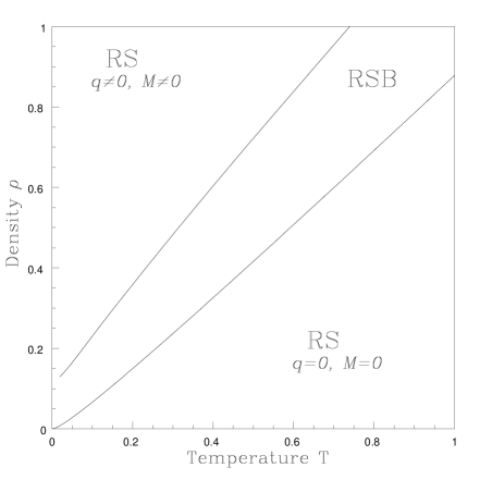
FIG. 1.: Phase diagram for the 3 dimensional RKKY interaction using Hartree approximation.

REFERENCES

- [1] Th. M. Nieuwenhuizen, Europhys. Lett., 24, 797 (1993).
- [2] M. Mézard, G. Parisi and Virasoro M. A., Spin Glass Theory and Beyond, Lecture Notes in Physics Vol. 9 (World Scientific, Singapore, 1987).
- [3] D.S. Fisher and D.A. Huse, Phys. Rev. Lett. 56, 1601 (1986); Phys. Rev. B 38, 386 (1988).
- [4] D.S. Dean and D.J. Lancaster in preparation.
- [5] V. Dotsenko, A.B. Harris, D. Sherrington and R.B. Stinchcombe, J.Phys. A. 28, 3093 (1995).
- [6] D.S. Dean and D.J. Lancaster in preparation.
- [7] M. Mézard and G. Parisi, J. Phys. I France 1, 809 (1991.)
- [8] D. Sherrington and S. Kirkpatrick, Phys. Rev. Lett., 35 1972 (1975); Phys. Rev. B 17, 4384 (1977).
- [9] J.R.L. de Almeida and D.J. Thouless, J.Phys. A, 11 983 (1978).
- [10] E. Pytte and J. Rudnick., Phys Rev B19, 3603 (1979).
- [11] G. Parisi, J. Phys. A 13, 164 (1980).
- [12] I. Kondor, C. De Dominicis and T. Temesvári, J.Phys. A 27, 7569 (1994).
- [13] The bounds given in [3] are for Ising spins.
- [14] D. Sherrington, Phys. Rev. B 22, 5553 (1980).
- [15] L. Viana and A.J. Bray, J.Phys. C 18, 3037 (1985).