Weak Antilocalization and Spin Precession in Quantum Wells

Abstract

The results of magnetoconductivity measurements in GaInAs quantum wells are presented. The observed magnetoconductivity appears due to the quantum interference, which lead to the weak localization effect. It is established that the details of the weak localization are controlled by the spin splitting of electron spectra. A theory is developed which takes into account both linear and cubic in electron wave vector terms in spin splitting, which arise due to the lack of inversion center in the crystal, as well as the linear terms which appear when the well itself is asymmetric. It is established that, unlike spin relaxation rate, contributions of different terms into magnetoconductivity are not additive. It is demonstrated that in the interval of electron densities under investigation ($(0.98-1.85)\cdot 10^{12}\ {\rm cm}^{-2}$) all three contribution are comparable and have to be taken into account to achieve a good agreement between the theory and experiment. The results obtained from comparison of the experiment and the theory have allowed us to determine what mechanisms dominate the spin relaxation in quantum wells and to improve the accuracy of determination of spin splitting parameters in ${\rm A}_{3}{\rm B}_{5}$ crystals and $2D$ structures.

]

I Introduction

The effect of the weak localization in metals and semiconductors is caused by the interference of two electron waves which are scattered by the same centers (defects or impurities) but propagate in opposite directions along the same closed trajectory, and, therefore, return to the origin with equal phases. This effect increases the effective scattering crossection, and, therefore, leads to a suppression of conductivity[3, 4, 5]. In a magnetic field, the two waves propagating in the opposite directions acquire a phase difference $2e\Phi/c$, where $\Phi$ is the magnetic flux through the area enclosed by the electron trajectory. This phase difference breaks the constructive interference and restores the conductivity to the value it would have without the quantum interference corrections. This is observed as an increase in conductivity with magnetic field, the effect known as positive magnetoconductivity (PMC) or negative magnetoresistance [6, 7].

When spin effects are taken into account, the interference depends significantly on the total spin of the two electron waves. The singlet state with the total spin $J=0$ gives negative contribution to the conductivity (antilocalization effect). The triplet state with $J=1$ gives positive contribution to the conductivity. In the absence of spin relaxation the contribution of the singlet state is canceled by one of triplet states. As a result, the magnetic field dependence of the conductivity is the same as for spinless particles. However, strong spin relaxation can suppress the triplet state contribution without changing that of the singlet state, hence the total quantum correction may become positive. The interplay between negative magnetoconductivity at low fields and positive magnetoconductivity at high fields can lead to appearance of a minimum on the conductivity – magnetic field curve (antilocalization minimum).

It was shown in the early papers by Hikami, Larkin, and Nagaoka[7] and by Altshuler, Aronov, Larkin, and Khmelnitskii[8] that the behavior of the conductivity in weak magnetic fields depends essentially on the mechanism of the spin relaxation. Three mechanisms were considered: Elliott-Yafet, otherwise known as skew scattering mechanism, scattering on paramagnetic impurities, and Dyakonov–Perel mechanism, which arises from the spin splitting of carrier spectra in non-centrosymmetric media.

Dyakonov–Perel mechanism is dominant in most ${\rm A}_{3}{\rm B}_{5}$ cubic semiconductors[9], with the exception of those with narrow band gap $E_{g}$ and large spin-orbit splitting of the valence band $\Delta$ (for example, InSb). The same can be said about the low-dimensional structures fabricated from these materials. Presence of a antilocalization minimum on the $\sigma(B)$ curves in quantum $2D$ systems is a definite sign that the dominant spin-relaxation mechanism is the Dyakonov–Perel one. It is known[7] that for the Elliott-Yafet mechanism in $2D$ structures the contribution of the singlet state with $J=0$ is exactly canceled by one of the triplet states, the one with $J=1$ and $J_{z}=0$.

Unlike bulk crystals, where the spin splitting is proportional to the cube of the wave vector $k$, in $2D$ structures the splitting has also terms linear in $k$ (this is also true for strained ${\rm A}_{3}{\rm B}_{5}$ crystals and for hexagonal ${\rm A}_{2}{\rm B}_{6}$ compounds). Furthermore, there are two linear in $k$ contributions of essentially different nature. The first one, which arises from the lack of inversion in the original crystal (like the cubic term), is known as Dresselhaus term[10], while the second, Rashba term, is caused by the asymmetry of the quantum well or heterojunction itself[11].

The direct measurements of the spin splitting using the Raman scattering in GaAs/AlGaAs quantum wells[12] have shown that, for electron densities $N_{s}\sim 10^{12}\ {\rm cm}^{-2}$, both linear contributions are comparable. All three terms give additive contributions to the spin relaxation rate. When only the cubic in $k$ term is present, its effect on the PMC is determined only by the spin relaxation rate, similarly to the two other spin relaxation mechanisms, and is described by the theory of Refs. [7, 8]. In the presence of the linear in $k$ term in the spin Hamiltonian it is necessary to take into account the correlations between the motion of electrons in the coordinate and spin spaces [13]. In the theory of coherent phenomena these correlations were first taken into account using the language of the spin-dependent vector potential in Refs. [14, 15, 16], where this concept was applied to consideration of spin-orbit conductance oscillations [14, 15] and of the spin orbit effects in the universal conductance fluctuation and persistent current in rings[16]. In the theory of the anomalous magnetoconductivity the correlation between motion in real and spin spaces was first taken into account in Ref. [17]. It was shown that when linear and cubic in $k$ terms are present, their contributions to spin phase-breaking are not additive. Furthermore, as it was demonstrated in Ref. [18], the contributions of Rashba and Dresselhaus terms are also nonadditive, and the magnetoconductivity is determined not by their sum, but rather their difference. Similar effect, when spin-orbit phase-breaking may become negligible due to the correlation of motion in real and spin spaces occurs in quasi-$1D$ case and leads to two types of pronounced oscillations in the universal conductance fluctuations in rings[19].

First experimental studies of the PMC in quantum $2D$ structures were done in Refs. [20, 21, 22]. Recently, the experimental observations of very pronounced effects of spin scattering on weak localization conductivity corrections in GaAs [23, 24] and InAs [25] heterostructures have been reported. Different spin relaxation mechanisms are invoked to explain the experimental data. In the Ref. [23] the spin relaxation is interpreted in the framework of the Dyakonov-Perel mechanism based on the bulk GaAs Hamiltonian. According to the authors, agreement with experimental data is achieved if one neglects in the spin-orbit Hamiltonian the term linear in the in-plane wave vector. This is in contradiction with the theoretical predictions[18] which show that, at least for low carrier concentrations, the linear term should be the dominant one. In Ref. [25] the same Dyakonov-Perel mechanism is used, but it is based on the Rashba term. In Ref. [24] it is assumed that the dominant mechanism of spin relaxation is the Elliott-Yafet scattering one. Recently, we have reported the measurements of the magnetoconductivity of GaInAs quantum wells[26]. We have used Altshuler-Aronov-Larkin-Khmelnitskii (AALKh) calculation [8] of quantum corrections to conductivity to interpret the experimental data. However, the spin relaxation time, which enters the AALKh expressions, was calculated taking into account not only linear but also cubic Dresselhaus terms of the spin splitting. We have demonstrated that, using this simplified theoretical approach, one can obtain right order of magnitude for the experimentally observed spin relaxation rates.

In this work we present detailed experimental study of the negative magnetoconductivity in selectively doped GaInAs quantum wells with different $2D$ carrier densities. We interpret them in the framework of recently developed theory of the anomalous magnetoconductivity in quantum wells which corrects the AALKh approach[17, 18]. Comparison of experiment and theory allows to determine importance of both Dresselhaus and Rashba terms for 2D systems.

II Theory

A Spin relaxation

The theory of the positive magnetoconductivity (PMC) for structures with spin splitting linear in wave vector was described very briefly in Refs. [17, 18]. Below we present an outline of this theory in more details. The spin splitting of the conduction band in cubic crystals ${\rm A}_{3}{\rm B}_{5}$ is described by the following Hamiltonian[10]:

$${\cal H}_{s}=\gamma\sum\sigma_{i}k_{i}\left(k_{i+1}^{2}-k_{i+2}^{2}\right),\quad i=x,y,z,\quad i+3\rightarrow i.$$ (1)

where $\sigma_{i}$ are the Pauli matrices. In $[001]$ quantum wells the size quantization gives rise to the terms in the Hamiltonian ${\cal H}_{s}$, which are linear in the in-plane wave vector $\mbox{\boldmath$k$}=(k_{x},k_{y})$, in addition to the cubic terms[8, 27]. The corresponding Hamiltonian for the conduction band electrons can be written as[17, 18]

$${\cal H}=\frac{k^{2}}{2m}+(\mbox{\boldmath$\sigma$}{\bf\Omega}),$$ (2)

where $\mbox{\boldmath$\sigma$}=(\sigma_{x},\sigma_{y})$, ${\bf\Omega}=(\Omega_{x},\Omega_{y})$ are two-dimensional vectors with components in the plane of the quantum well. Vector $2{\bf\Omega}/\hbar$ has the physical meaning of the precession vector: its length equals the frequency of the spin precession and its direction defines the axis of the precession. The spin splitting energy is equal to $2\Omega$. To treat the spin relaxation problem in the case when $\Omega$ is anisotropic in the $2D$ plane one has to decompose it into orthogonal spherical harmonics:

$${\bf\Omega} = {\bf\Omega}_{1}+{\bf\Omega}_{3},$$ (3)

$$\Omega_{1x} = -\Omega_{1}^{(1)}\cos\varphi,\ \Omega_{3x}=-\Omega_{3}\cos 3\varphi,$$ (4)

$$\Omega_{1y} = \ \Omega_{1}^{(1)}\sin\varphi,\ \Omega_{3y}=-\Omega_{3}\sin 3\varphi,$$ (5)

$$\Omega_{1}^{(1)} = \gamma k\left(\left\langle k_{z}^{2}\right\rangle-{1\over 4}k^{2}\right),\quad\Omega_{3}=\gamma{k^{3}\over 4},$$ (6)

where $k^{2}=k_{x}^{2}+k_{y}^{2}$, $\tan\varphi=k_{x}/k_{y}$, and $\left\langle k_{z}^{2}\right\rangle$ is the average squared wave vector in the direction $z$, normal to the quantum well (in this paper we take $\hbar=1$ everywhere except in final formulas).

The spin splitting given by Eq. (5) represents the Dresselhaus term[10]. In asymmetric quantum wells the Hamiltonian ${\cal H}$ contain also terms of different symmetry, i.e. the Rashba terms[11]:

$$H^{\prime}=\alpha[\mbox{\boldmath$\sigma k$}]_{z}.$$ (7)

This term can be included in the Hamiltonian Eq. (2) if one includes additional terms into ${\bf\Omega}$:

$$\Omega_{1x}=\Omega_{1}^{(2)}\sin\varphi,\quad\Omega_{1y}=-\Omega_{1}^{(2)}\cos\varphi,\quad\Omega_{1}^{(2)}=\alpha k.$$ (8)

In an uniform electric field ${\cal E}$, the constant $\alpha$ is proportional to the field:

$$\alpha=\alpha_{0}e{\cal E}.$$ (9)

The expressions for $\alpha_{0}$ and $\gamma$ are given in the Appendix. The barriers of the well give rise to another contribution, usually also linear in ${\cal E}$, which depends strongly on the details of the boundary conditions at the heterointerface[28, 29].

Both terms Eqs. (5) and (8) give additive contributions to the spin relaxation rate $1/\tau_{ij}$, which is defined as

$$\frac{ds_{i}}{dt}=-\frac{s_{j}}{\tau_{ij}}.$$ (10)

where $s_{i}$ is an average projection of spin on the direction $i$. These contributions are

$${1\over\tau_{s_{xx}}}={1\over 2\tau_{s_{zz}}}=2\left(\Omega_{1}^{2}\tau_{1}+\Omega_{3}^{2}\tau_{3}\right),$$ (11)

where $\Omega_{1}^{2}={\Omega_{1}^{(1)}}^{2}+{\Omega_{1}^{(2)}}^{2}$ and $\tau_{n}$, $n=1,3$, is the relaxation time of the respective component of the distribution function $f_{n}(\mbox{\boldmath$k$})\sim\cos n(\varphi_{\mbox{\boldmath$k$}}+\psi_{n})$ ($\psi_{n}$ is an arbitrary phase):

$${1\over\tau_{n}}=\int W(\varphi)\left(1-\cos n\varphi\right)\,d\varphi.$$ (12)

Here $W(\vartheta)$ is the probability of scattering by an angle $\vartheta$. If it does not depend on $\vartheta$, all scattering times are equal to the elastic lifetime

$$\frac{1}{\tau_{0}}=\int W(\varphi)\,d\varphi.$$ (13)

When small-angle scattering dominates, $1-\cos n\varphi\approx(n\varphi)^{2}/2$ and

$$\frac{\tau_{1}}{\tau_{n}}=n^{2},\qquad(n\geq 1).$$ (14)

Formula Eq. (11) shows that the different harmonics of the precession vector add up in the spin relaxation rate with the weight equal to the relaxation times $\tau_{n}$. Unlike the spin relaxation, the contributions of the different terms in the spin splitting into PMC are not additive. Furthermore, at $\Omega_{1}^{(1)}=\pm\Omega_{1}^{(2)}$ and $\Omega_{3}=0$ the contributions of the two linear terms Eqs. (5) and (8) exactly cancel each other, and the magnetoconductivity looks as if there were no spin-orbit interaction at all. Analogous effect occur in weak localization conductance in wires[16].

B Weak localization in two-dimensional structures

The weak localization contribution to the conductivity is given by the expression[7, 8]:

$$\Delta\sigma=-{e^{2}D\over\pi}\cdot 2\pi\nu_{0}\tau_{0}^{2}\sum_{\alpha\beta}\int\limits_{0}^{q_{max}}{{\rm\kern 2.40005pt\vrule width=0.50003pt,height=6.02773pt,depth=-0.21529pt\kern-2.59995ptC}}_{\alpha\beta\beta\alpha}(\mbox{\boldmath$q$})\,\frac{d^{2}q}{(2\pi)^{2}},$$ (15)

where $\alpha$ and $\beta$ are spin indices, $q_{max}^{2}=(D\tau_{1})^{-1}$, $D=v^{2}\tau_{1}/2$ is the diffusion coefficient, and $\nu_{0}=m/2\pi$ is the density of states at the Fermi level at a given spin projection. The matrix ${{\rm\kern 2.40005pt\vrule width=0.50003pt,height=6.02773pt,depth=-0.21529pt\kern-2.59995ptC}}_{\alpha\beta\beta\alpha}(\mbox{\boldmath$q$})$ is called Cooperon and can be found from the following integral equation:

$${{\rm\kern 2.40005pt\vrule width=0.50003pt,height=6.02773pt,depth=-0.21529pt\kern-2.59995ptC}}_{\alpha\beta\gamma\delta}(\mbox{\boldmath$k$},\mbox{\boldmath$k$}^{\prime},\mbox{\boldmath$q$})=\left|V_{\mbox{\boldmath$k$},\mbox{\boldmath$k$}^{\prime}}\right|^{2}\delta_{\alpha\gamma}\delta_{\beta\delta}$$ (16)

$$+ \int\frac{d^{2}g}{(2\pi)^{2}}\sum_{\lambda\lambda^{\prime}}V_{\mbox{\boldmath$k$},\mbox{\boldmath$g$}}V_{-\mbox{\boldmath$k$},-\mbox{\boldmath$g$}}G^{+}_{\alpha\lambda}(\omega,\mbox{\boldmath$g$}+\mbox{\boldmath$q$})G^{-}_{\beta\lambda^{\prime}}(\omega,-\mbox{\boldmath$g$})$$ (17)

$$\times {{\rm\kern 2.40005pt\vrule width=0.50003pt,height=6.02773pt,depth=-0.21529pt\kern-2.59995ptC}}_{\lambda\lambda^{\prime}\gamma\delta}(\mbox{\boldmath$g$},\mbox{\boldmath$k$}^{\prime},\mbox{\boldmath$q$}).$$ (18)

Here $V_{\mbox{\boldmath$k$},\mbox{\boldmath$k$}^{\prime}}$ is a scattering matrix element (including the concentration of scatterers), which we assume here to be diagonal in spin indices. It is connected with $W(\varphi)$ in Eq. (13) by the expression

$$W\left(\varphi_{\mbox{\boldmath$k$}}-\varphi_{\mbox{\boldmath$k$}^{\prime}}\right)=\nu_{0}\left|V_{\mbox{\boldmath$k$},\mbox{\boldmath$k$}^{\prime}}\right|^{2},$$ (19)

$G^{\pm}(\omega,\mbox{\boldmath$k$})$ are the Green’s functions

$$G^{\pm}(\omega,\mbox{\boldmath$k$})=\left\{\omega-E(k)-(\mbox{\boldmath$\sigma$}{\bf\Omega})\pm\frac{i}{\tau_{f}}\right\}^{-1},$$ (20)

$$\frac{1}{\tau_{f}}=\frac{1}{\tau_{0}}+\frac{1}{\tau_{\varphi}},\qquad E(k)=\frac{k^{2}}{2m},$$ (21)

$\tau_{\varphi}$ is the inelastic scattering time. After the integration by $E(g)$ in the right-hand side of Eq. (16) the result is expanded up to second order terms in series in small parameters $\tau_{0}/\tau_{\varphi}$, $\mbox{\boldmath$vq$}\tau_{0}$, and $\Omega\tau_{0}$, where $\mbox{\boldmath$v$}=\partial E/\partial\mbox{\boldmath$k$}$. In the end, the following equation for the Cooperon is obtained:

$${{\rm\kern 2.40005pt\vrule width=0.50003pt,height=6.02773pt,depth=-0.21529pt\kern-2.59995ptC}}_{\mbox{\boldmath$k$},\mbox{\boldmath$k$}^{\prime}}(\mbox{\boldmath$q$})=\left|V_{\mbox{\boldmath$k$},\mbox{\boldmath$k$}^{\prime}}\right|^{2}+2\pi\nu_{0}\tau_{0}\int\frac{d\varphi_{g}}{2\pi}\left|V_{\mbox{\boldmath$k$},\mbox{\boldmath$g$}}\right|^{2}$$ (22)

$$\times\Bigg{\{}1-i(\mbox{\boldmath$v$}_{g}\mbox{\boldmath$q$})\tau_{0}-i(\mbox{\boldmath$\sigma$}+\mbox{\boldmath$\rho$}){\bf\Omega}\tau_{0}-(\mbox{\boldmath$v$}_{g}\mbox{\boldmath$q$})^{2}\tau_{0}^{2}$$ (23)

$$-2(\mbox{\boldmath$\sigma$}{\bf\Omega})((\mbox{\boldmath$\rho$}{\bf\Omega})\tau_{0}^{2}-2(\mbox{\boldmath$v$}_{g}\mbox{\boldmath$q$})(\mbox{\boldmath$\sigma$}+\mbox{\boldmath$\rho$}){\bf\Omega}\tau_{0}^{2}-\frac{\tau_{0}}{\tau_{\varphi}}\Bigg{\}}{{\rm\kern 2.40005pt\vrule width=0.50003pt,height=6.02773pt,depth=-0.21529pt\kern-2.59995ptC}}_{\mbox{\boldmath$g$},\mbox{\boldmath$k$}^{\prime}}(\mbox{\boldmath$q$}).$$ (24)

Here the Pauli matrices $\sigma$ act on the first pair of spin indices $\alpha,\lambda$, while the matrices $\rho$– on the second pair $\beta\lambda^{\prime}$.

The equation

$${{\rm\kern 2.40005pt\vrule width=0.50003pt,height=6.02773pt,depth=-0.21529pt\kern-2.59995ptC}}_{\mbox{\boldmath$k$},\mbox{\boldmath$k$}^{\prime}}=\lambda\tau_{0}\int W(\mbox{\boldmath$k$}^{\prime},\mbox{\boldmath$g$}){{\rm\kern 2.40005pt\vrule width=0.50003pt,height=6.02773pt,depth=-0.21529pt\kern-2.59995ptC}}_{\mbox{\boldmath$g$},\mbox{\boldmath$k$}^{\prime}}d\varphi_{g}$$ (25)

has the following harmonics as its eigenfunctions:

$${{\rm\kern 2.40005pt\vrule width=0.50003pt,height=6.02773pt,depth=-0.21529pt\kern-2.59995ptC}}^{n}_{\mbox{\boldmath$k$},\mbox{\boldmath$k$}^{\prime}}={{\rm\kern 2.40005pt\vrule width=0.50003pt,height=6.02773pt,depth=-0.21529pt\kern-2.59995ptC}}^{n}.\cos n(\varphi_{k}-\varphi_{k^{\prime}}-\psi_{n})$$ (26)

According to Eq. (13) the eigenfunction ${{\rm\kern 2.40005pt\vrule width=0.50003pt,height=6.02773pt,depth=-0.21529pt\kern-2.59995ptC}}_{0}$ has the eigenvalue $\lambda_{0}=1$, while other harmonics have eigenvalues

$$\lambda_{n}=\left(1-\frac{\tau_{0}}{\tau_{n}}\right)^{-1}.$$ (27)

Therefore, the solution of inhomogeneous equation Eq. (23) will have large harmonic ${{\rm\kern 2.40005pt\vrule width=0.50003pt,height=6.02773pt,depth=-0.21529pt\kern-2.59995ptC}}_{0}$, while the others will be small, because they appear due to presence of small terms in $q$ and $\Omega$. Since the right-hand side of Eq. (23) contains linear and cubic in $g$ terms, in is necessary to take into account only first and third harmonics. From Eqs. (23) – (27) it follows that

$${{\rm\kern 2.40005pt\vrule width=0.50003pt,height=6.02773pt,depth=-0.21529pt\kern-2.59995ptC}}^{(1)}_{\mbox{\boldmath$g$},\mbox{\boldmath$k$}^{\prime}} = -i(\tau_{1}-\tau_{0})\left[(\mbox{\boldmath$v$}_{g}\mbox{\boldmath$q$})+(\mbox{\boldmath$\sigma$}+\mbox{\boldmath$\rho$}){\bf\Omega}_{1}(\mbox{\boldmath$g$})\right]{{\rm\kern 2.40005pt\vrule width=0.50003pt,height=6.02773pt,depth=-0.21529pt\kern-2.59995ptC}}^{0}_{\mbox{\boldmath$g$},\mbox{\boldmath$k$}^{\prime}}$$ (28)

$${{\rm\kern 2.40005pt\vrule width=0.50003pt,height=6.02773pt,depth=-0.21529pt\kern-2.59995ptC}}^{(3)}_{\mbox{\boldmath$g$},\mbox{\boldmath$k$}^{\prime}} = -i(\tau_{3}-\tau_{0})(\mbox{\boldmath$\sigma$}+\mbox{\boldmath$\rho$}){\bf\Omega}_{3}(\mbox{\boldmath$g$}){{\rm\kern 2.40005pt\vrule width=0.50003pt,height=6.02773pt,depth=-0.21529pt\kern-2.59995ptC}}^{0}_{\mbox{\boldmath$g$},\mbox{\boldmath$k$}^{\prime}}$$ (29)

Here it is taken into account that there is a relation similar to Eq. (25) for harmonics $\Omega_{1\alpha}$, $(\mbox{\boldmath$v$}\mbox{\boldmath$q$})\sim\cos(\varphi_{\mbox{\boldmath$g$}}-\varphi_{\mbox{\boldmath$q$}})$, and $\Omega_{3\alpha}$.

Then we substitute ${{\rm\kern 2.40005pt\vrule width=0.50003pt,height=6.02773pt,depth=-0.21529pt\kern-2.59995ptC}}_{\mbox{\boldmath$g$},\mbox{\boldmath$k$}^{\prime}}={{\rm\kern 2.40005pt\vrule width=0.50003pt,height=6.02773pt,depth=-0.21529pt\kern-2.59995ptC}}^{0}_{\mbox{\boldmath$g$},\mbox{\boldmath$k$}^{\prime}}+{{\rm\kern 2.40005pt\vrule width=0.50003pt,height=6.02773pt,depth=-0.21529pt\kern-2.59995ptC}}^{(1)}_{\mbox{\boldmath$g$},\mbox{\boldmath$k$}^{\prime}}+{{\rm\kern 2.40005pt\vrule width=0.50003pt,height=6.02773pt,depth=-0.21529pt\kern-2.59995ptC}}^{(3)}_{\mbox{\boldmath$g$},\mbox{\boldmath$k$}^{\prime}}$ into Eq. (23), and, using Eq. (29) and retaining only the terms with zero harmonic, we obtain the equation for ${{\rm\kern 2.40005pt\vrule width=0.50003pt,height=6.02773pt,depth=-0.21529pt\kern-2.59995ptC}}_{0}(\mbox{\boldmath$q$})$:

$${\cal H}{{\rm\kern 2.40005pt\vrule width=0.50003pt,height=6.02773pt,depth=-0.21529pt\kern-2.59995ptC}}_{0}={1\over 2\pi\nu_{0}\tau_{0}^{2}},$$ (30)

where

$${\cal H}= {1\over\tau_{\varphi}}+{1\over 2}v^{2}q^{2}\tau_{1}+$$ (35)

$$\left(\Omega_{1}^{2}\tau_{1}+\Omega_{3}^{2}\tau_{3}\right)\left(2+\sigma_{x}\rho_{x}+\sigma_{y}\rho_{y}\right)+$$

$$2\left(\sigma_{x}\rho_{y}+\sigma_{y}\rho_{x}\right)\Omega_{1}^{(1)}\Omega_{1}^{(2)}\tau_{1}+$$

$$v\tau_{1}\left[\left(\sigma_{x}+\rho_{x}\right)\left(-\Omega_{1}^{(1)}q_{x}+\Omega_{1}^{(2)}q_{y}\right)+\right.$$

$$\left.\left(\sigma_{y}+\rho_{y}\right)\left(\Omega_{1}^{(1)}q_{y}-\Omega_{1}^{(2)}q_{x}\right)\right].$$

In a magnetic field $q$ become operators with the commutator

$$[q_{+}q_{-}]={\delta\over D},$$ (36)

where $q_{\pm}=q_{x}\pm iq_{y}$ and

$$\delta={4eBD\over\hbar c}.$$ (37)

This allows us to introduce creation and annihilation operators $a^{\dagger}$ and $a$, respectively, for which $[aa^{\dagger}]=1$:

$$D^{1/2}q_{+}=\delta^{1/2}a,\quad D^{1/2}q_{-}=\delta^{1/2}a^{\dagger},\quad Dq^{2}=\delta\{aa^{\dagger}\}.$$ (38)

In the basis of the eigenfunction of the operator $\{aa^{\dagger}\}={1\over 2}(aa^{\dagger}+a^{\dagger}a)$ these operators have following non-zero matrix elements

$$\left\langle n-1\right|a\left|n\right\rangle = \left\langle n\right|a^{\dagger}\left|n-1\right\rangle=\sqrt{n},$$ (39)

$$\left\langle n\right|\{aa^{\dagger}\}\left|n\right\rangle = n+{1\over 2}.$$ (40)

In a magnetic field, the integration over $q$ should be replaced by summation over $n$. Then,

$$\Delta\sigma=-\frac{e^{2}\delta}{4\pi^{2}\hbar}S,$$ (41)

where

$$S=2\pi\nu_{0}\tau_{0}^{2}\sum_{\alpha,\beta,n}{{\rm\kern 2.40005pt\vrule width=0.50003pt,height=6.02773pt,depth=-0.21529pt\kern-2.59995ptC}}_{\alpha\beta\beta\alpha}(n).$$ (42)

Since Eq. (30) is essentially the Green function equation its solution can be written as:

$${{\rm\kern 2.40005pt\vrule width=0.50003pt,height=6.02773pt,depth=-0.21529pt\kern-2.59995ptC}}(n)^{\alpha\gamma}_{\beta\delta}=\frac{1}{2\pi\nu_{0}\tau_{0}^{2}}\sum_{r=1}^{4}\frac{1}{E_{r,n}}\Psi_{r,n}(\alpha,\beta)\Psi_{r,n}^{*}(\gamma,\delta),$$ (43)

where $\Psi_{r,n}$ and $E_{r,n}$ are the eigenfunctions and eigenvalues of ${\cal H}$:

$${\cal H}\Psi_{r,n}=E_{r,n}\Psi_{r,n}.$$ (44)

We now choose the basis consisting of the function $\Psi_{0}(\alpha,\beta)$, which is antisymmetric in spin indices and corresponds to the total momentum $J=0$, and of symmetric functions $\Psi_{m}$ which correspond to $J=1$ and $J_{z}=m=-1,\ 0,\ 1$. According to Eq. (43), in this basis the sum in Eq. (41) is

$$S=\sum_{n=0}^{n_{max}}\left(-{1\over E_{0}(n)}+\sum_{m=-1}^{1}{1\over E_{m}(n)}\right),$$ (45)

where $n_{max}=1/\delta\tau_{1}$. For the term with $J=0$ the operator ${\cal H}$ is

$${\cal H}_{0n}=\delta\{aa^{\dagger}\}+\frac{1}{\tau_{\varphi}},$$ (46)

and, therefore,

$$E_{0}(n)=\delta\left(n+{1\over 2}\right)+{1\over\tau_{\varphi}}.$$ (47)

For the term with $J=1$ we can use the relation $J_{i}=(\sigma_{i}+\rho_{i})/2$ to obtain

$$\tilde{\cal H}= \delta\{aa^{\dagger}\}+{1\over\tau_{\varphi}}+2\left(\Omega_{1}^{2}\tau_{1}+\Omega_{3}^{2}\tau_{3}\right)\left(2-J_{z}^{2}\right)-$$ (50)

$$4i\Omega_{1}^{(1)}\Omega_{1}^{(2)}\tau_{1}\left(J_{+}^{2}-J_{-}^{2}\right)+2(\delta\tau_{1})^{1/2}$$

$$\times\left[-\Omega_{1}^{(1)}\left(J_{+}a+J_{-}a^{\dagger}\right)+i\Omega_{1}^{(2)}\left(J_{+}a^{\dagger}-J_{-}a\right)\right].$$

where $J_{\pm}=(J_{x}\pm iJ_{y})/\sqrt{2}$.

When $\Omega_{1}^{(2)}=0$ (or $\Omega_{1}^{(1)}=0$), the operator Eq. (50) can be reduced to a block-diagonal form with $3\times 3$ blocks if one uses the basis of functions $\Psi_{n}={\bf(}f_{1}(n)F_{n-1},f_{0}(n)F_{n},f_{-1}(n)F_{n+1}{\bf)}$, where $F_{n}$ are the eigenfunctions of the operator $\{aa^{\dagger}\}$ and $f_{m}$ are the eigenfunctions of $J_{z}$ (for $\Omega_{1}^{(1)}=0$ the basis is $\Psi_{n}={\bf(}f_{1}(n)F_{n+1},f_{0}(n)F_{n},f_{-1}(n)F_{n-1}{\bf)}$). Using the formula

$$\sum_{m}\frac{1}{E_{m}}=\sum_{m}\frac{\left|D_{mm}\right|}{|D|},$$ (51)

where $|D|$ is the determinant of ${\cal H}$ (Eq. (50)) and $\left|D_{mm}\right|$ are its minors of diagonal elements $D_{mm}$, the sum in Eq. (45) can be immediately calculated[17]. According to Eqs. (41), (50), and (51),

$$\Delta \sigma(B)=-\frac{e^{2}}{4\pi^{2}\hbar}\Biggl{\{}\frac{1}{a_{0}}+\frac{2a_{0}+1+\frac{H_{SO}}{B}}{a_{1}\left(a_{0}+\frac{H_{SO}}{B}\right)-2\frac{H^{\prime}_{SO}}{B}}$$ (55)

$$-\sum_{n=0}^{\infty}\Biggl{(}\frac{3}{n}$$

$$-\frac{3a_{n}^{2}+2a_{n}\frac{H_{SO}}{B}-1-2(2n+1)\frac{H^{\prime}_{SO}}{B}}{\left(a_{n}+\frac{H_{SO}}{B}\right)a_{n-1}a_{n+1}-2\frac{H^{\prime}_{SO}}{B}\left[(2n+1)a_{n}-1\right]}\Biggr{)}$$

$$+2\ln\frac{H_{tr}}{B}+\Psi\left(\frac{1}{2}+\frac{H_{\varphi}}{B}\right)+3C\Biggr{\}},$$

where $C$ is the Euler’s constant,

$$a_{n} = n+\frac{1}{2}+\frac{H_{\varphi}}{B}+\frac{H_{SO}}{B},$$ (56)

$$H_{\varphi} = {c\over 4e\hbar D\tau_{\varphi}},\ {B\over H_{\varphi}}=\delta\tau_{\varphi},\ H_{tr}={c\over 4e\hbar D\tau_{1}},$$ (57)

$$H_{SO} = {c\over 4\hbar eD}\left(2\Omega_{1}^{2}\tau_{1}+2\Omega_{3}^{2}\tau_{3}\right),\ H^{\prime}_{SO}=H^{(1)}_{SO}{\rm\ or\ }H^{(2)}_{SO},$$ (58)

$$H^{(1)}_{SO} = {c\over 4\hbar eD}{2\Omega_{1}^{(1)}}^{2}\tau_{1},\ H^{(2)}_{SO}={c\over 4\hbar eD}{2\Omega_{1}^{(2)}}^{2}\tau_{1},$$ (59)

and $\Psi$ is a digamma-function.

If both $\Omega_{1}^{(1)}=\Omega_{1}^{(2)}=0$ and only the cubic in $k$ term with $\Omega_{3}$ is present, the expression Eq. (55) can be further reduced to the formula, which was obtained earlier in Ref. [8]:

$$\Delta \sigma(B)-\Delta\sigma(0)=\frac{e^{2}}{2\pi^{2}\hbar}\Biggl{\{}\Psi\left(\frac{1}{2}+\frac{H_{\varphi}}{B}+\frac{H_{SO}}{B}\right)+$$ (62)

$$\frac{1}{2}\Psi\left(\frac{1}{2}+\frac{H_{\varphi}}{B}+2\frac{H_{SO}}{B}\right)-\frac{1}{2}\Psi\left(\frac{1}{2}+\frac{H_{\varphi}}{B}\right)-$$

$$\ln\frac{H_{\varphi}+H_{SO}}{B}-\frac{1}{2}\ln\frac{H_{\varphi}+2H_{SO}}{B}+\frac{1}{2}\ln\frac{H_{\varphi}}{B}\Biggr{\}}.$$

Note that, according to Ref. [17], the value of $H_{SO}$ is twice that used in Ref. [8].

The case when $\Omega_{1}^{(1)}=\pm\Omega_{1}^{(2)}$ and $\Omega_{3}=0$ is a special one. In this case the operator Eq. (35) is diagonal in the basis of functions $\Psi_{m}$ if one uses coordinates $x^{\prime}\parallel(110)$ and $y^{\prime}\parallel(1\bar{1}0)$:

$${\cal H}_{mm^{\prime}}=\left\{\frac{1}{\tau_{\varphi}}+D\left[q_{x^{\prime}}^{2}+\left(q_{y^{\prime}}+q_{y^{\prime}m}^{0}\right)^{2}\right]\right\}\delta_{mm^{\prime}},$$ (63)

where $q_{y^{\prime}m}^{0}=2\Omega_{1}\sqrt{\tau_{1}/D}m$. Since the commutation relations Eq. (36) do not change when $q_{y^{\prime}}$ is shifted by $q_{y^{\prime}}^{0}$, the spin splitting does not manifest itself in the magnetoconductivity, which is given by the simple formula[7]

$$\Delta\sigma(B)-\Delta\sigma(0)=\frac{e^{2}}{2\pi^{2}\hbar}\left\{\Psi\left(\frac{1}{2}+\frac{H_{\varphi}}{B}\right)-\ln\frac{H_{\varphi}}{B}\right\}.$$ (64)

It was demonstrated in Ref. [18] that this result appears because, when $\Omega_{1}^{(1)}=\pm\Omega_{1}^{(2)}$ and $\Omega_{3}=0$, the total spin rotation for the motion along any closed trajectory is exactly zero.

When $\Omega_{1}^{(1)}$ and $\Omega_{1}^{(2)}$ are not equal or $\Omega_{3}\neq 0$, the only way to find eigenvalues $E_{mn}$ is to diagonalize numerically the matrix $\tilde{\cal H}$. The number of elements one has to take for a given value of magnetic field $B$, or $\delta$, is at least $n_{max}=1/\delta\tau_{1}$ and increases infinitely as $B$ approaches $\mathrm{𝟎}$. Note that the size of the matrix $\tilde{\cal H}$ is $N=3n_{max}$. For the detail of the numerical procedure, see Ref. [18].

C Elliott-Yafet spin relaxation mechanism

It follows from Ref. [7] that in order to take into account the Elliott-Yafet spin relaxation mechanism one has to add a new term to the Hamiltonian Eq. (50):

$${\cal H}_{EY}=\frac{1}{\tau_{s_{EY}}}J_{z}^{2},$$ (65)

where, according to Ref. [9],

$$\frac{1}{\tau_{s_{EY}}} = \frac{1}{\tau_{2}}\left(\kappa^{2}\beta\right)^{2},$$ (66)

$$\beta = \frac{\hbar^{2}}{3m}\frac{\Delta\left(E_{g}-\frac{\Delta}{2}\right)}{E_{g}^{2}\left(E_{g}-\frac{\Delta}{3}\right)},$$ (67)

and $\tau_{2}$ is defined by Eq. (12).

As a result, in the first and fourth terms of the formula for magnetoconductivity Eq. (62) $H_{SO}$ should be replaced by $H_{SO}+H_{EY}$, where $H_{EY}$ is

$$H_{EY}=\frac{c}{4\hbar eD\tau_{s_{EY}}}.$$ (68)

It follows from Eq. (66) that

$$\frac{H_{EY}}{H_{tr}}=\left(2\pi N_{s}\beta\right)^{2}\,\frac{\tau_{1}}{\tau_{2}}.$$ (69)

III Experimental Procedures

A Samples

FIG. 1.: Sample structure (a) and band diagram (b) for GaInAs quantum well (sample B1) as obtained from self-consistent calculations. The first two energy levels in the well are shown by solid lines, Fermi energy is shown by a dotted line.

FIG. 2.: Energies determining the Dresselhaus spin splitting as a function of electron density $N_{s}$. Fermi energy $E_{F}$ and quadrupled mean kinetic energy $4E_{Z}$ of the motion in the growth direction are shown by solid lines. Dotted line shows the difference $4E_{Z}-E_{F}$ that enters Eq. (57) for $H^{(1)}_{SO}$.

TABLE I.: Sample parameters: electron density $N_{s}$, mobility $\mu$, transport magnetic field $H_{tr}$ (Eq. (57), and momentum relaxation time $\tau_{1}$.

$N_{s}{\ \rm(10^{12}\ cm^{-2})}$	$\mu{\ \rm(m^{2}/Vs)}$	$H_{tr}$ (Gs)	$\tau_{1}$ (ps)	sample	spacer
0.98	2.96	14	1.2	A1	6 nm
1.1	3.72	7.9	1.5	A2	6 nm
1.15	4.11	6.2	1.7	A3	6 nm
1.34	1.94	24	0.8	B1	4 nm
1.61	1.85	22	0.8	C1	2 nm
1.76	1.63	26	0.7	C2	2 nm
1.79	1.57	27	0.7	C3	2 nm
1.85	1.43	32	0.6	C4	2 nm

Three AlGaAs/InGaAs/GaAs pseudomorphic quantum wells were studied. They were grown by the molecular beam epitaxy technique. The layer sequence of the structure was of the standard HEMT type and is shown in Fig. 1. The two-dimensional electron gas was formed in the 13 nm thick InGaAs layer. Samples were $\delta$-doped with Si (doping density $N_{d}=2.5\cdot 10^{12}\ {\rm cm}^{-2})$. Samples of the type A had a spacer thickness of 6 nm, samples of the type B had a 4 nm spacer and samples of the type C had a 2nm spacer. The samples had the Hall bar geometry with the length of 1.0 mm and the width of 0.1 mm with two current and four voltage probes. The distance between voltage probes was 0.3 mm. The samples were independently characterized by luminescence, high field transport, and cyclotron emission experiments[30]. The parameters are listed in Table I. In order to study the behavior of the structures as a function of electron density $N_{s}$, the metastable properties of the DX-Si centers present in AlGaAs layer were employed. Different concentrations were obtained by cooling sample slowly in dark and then by illuminating it gradually by a light-emitting diode. This allowed us to tune carrier density from $0.98\cdot 10^{12}\ {\rm cm}^{-2}$ to $1.95\cdot 10^{12}\ {\rm cm}^{-2}$. We have measured the Hall effect and Shubnikov-de-Haas oscillations to determine $N_{s}$ and to verify that in all samples only the lowest subband is occupied. To calculate the energy levels in investigated quantum wells we first self-consistently calculate the $2D$ wavefunctions, using the envelope function approach in the Hartree approximation[31, 32]. The potential entering into the zero-magnetic field Hamiltonian takes into account the conduction band offset at each interface, and includes, in a self-consistent way, the electrostatic potential curvature due to the finite extent of the electron wavefunction. The boundary condition for the integration of Poisson equation within the $2D$ channel is the value of the built-in electric field in the buffer layer on the substrate side of the $2D$ channel. It originates from the pinning of the Fermi level near midgap in semiinsulating GaAs substrate. Any nonparabolicity effects on the effective masses were neglected. The calculations were performed for the temperature 4.2 K. Results of calculations are shown in Fig. 1. With increasing concentration both Fermi energy and kinetic energy of the motion in the growth direction increase. Their exact concentration dependencies should be determined to calculate spin splitting and spin relaxation times. For every carrier density $N_{s}$ the expectation value of the $z$-component of the kinetic energy was calculated. Figure 2 shows the result of such calculations for the quantum wells used in our experiments. We also show the Fermi energy as a function of carrier density $N_{s}$.

B Magnetic field generation and stability

We have used a system of two superconducting coils (8T/8T) placed in the same cryostat. This system was earlier used to study cyclotron emission from the same samples A, B, and C and to determine their effective masses[33]. The sample was placed in the center of the first coil. To generate the stable weak magnetic field, necessary for the antilocalization measurements we used a spread field of the second coil to compensate the field in the first one. The magnetic field scale was determined on the basis of measurements of the Hall voltages induced on the sample by both coils. Typically the constant magnetic field in the sample coil was of the order of 400 Gauss and it was compensated by tuning the second coil field in the range from 12 to 14 kGauss. This way, both coils were operated in a stable and reproducible manner giving in the sample space magnetic fields from - 30 Gauss to +30 Gauss. Small sample dimensions and the geometry of the coils gave good magnetic field uniformity. We estimate thet the magnetic field have varied by less than 0.1 Gauss over the sample.

C Conductivity measurements and temperature control

We have used the standard direct current (DC) method to measure the conductivity with currents less than 20 microampers to avoid sample heating. A high precision voltmeter capable of measuring nV changes on mV signals was used to measure the conductivity and Hall voltages. The whole system was computer controlled. To avoid mechanical and temperature instabilities, the sample was not directly immersed in the liquid helium but was enclosed in the vacuum tight sample holder and cooled by helium exchange gas under the 50 mbar pressure. A calibrated Allan–Bradley resistor placed near the sample was used to measure the temperature which was stabilized between 4.2K and 4.3K. The experimental arrangement allowed simultaneous complementary Shubnikov-de Haas and Hall effect measurements to determine carrier mobility and concentration for different sample illumination intensities.

IV Results and Discussion

A General comments

For all samples and for all carrier densities, the magnetoconductivity was a non-monotonic function of the magnetic field. As we have mentioned before, presence of a minimum on the $\sigma(B)$ curves is a definite sign that the dominant spin-relaxation mechanism is the Dyakonov–Perel one. For the Elliott-Yafet mechanism in $2D$ structures, the contribution of the singlet state with $J=0$ is exactly canceled by one of the triplet states, namely the one with $J=1$ and $J_{z}=0$, which is immediately evident from Eq. (65). Using Eq. (69) one can show that even for the highest density $N_{s}=2\cdot 10^{12}{\rm\ cm^{-2}}$ and $\tau_{1}/\tau_{2}=4$, the characteristic magnetic field $H_{EY}$ does not exceed $4\cdot 10^{-4}\,H_{tr}$, which is much smaller than $H_{SO}$. For the scattering on paramagnetic impurities, the negative magnetoconductivity at lowest fields does not exist both in $2D$ and $3D$ systems.

As we have already noted, the theory presented in this paper uses the diffusion approximation, which is valid only when all of the fields $H_{\varphi}$ and $H_{SO}$ are smaller than $H_{tr}$. Kinetic theory, which is free from this limitation, was developed in Refs. [34, 35, 36, 37] for the case of isotropic scattering and with spin relaxation considered in the framework of AALKh theory. The comparison with the diffusion theory shows that in magnetic field $B=0.4H_{tr}$ the latter has an error of 6%[37]. For the purpose of comparison with theory, we have selected only samples with $B$ at the minimum of $\sigma$ smaller than $0.4H_{tr}$.

B Description of fitting procedure

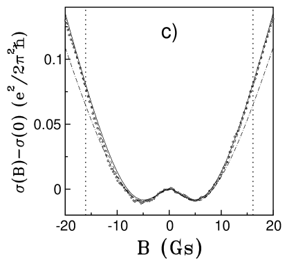
FIG. 3.: Experimental results (circles) and theoretical fits for the magnetoconductivity $\sigma(B)-\sigma(0)$ for three different samples: a) – A1, b) – B1, and c) – C4. Solid lines show results of the theory outlined in Sec. II. Best fits obtained from Eqs. (55) and (62) are shown by dashed and dotted-dashed lines, respectively. Dotted vertical lines show the values $B=0.5H_{tr}$, which limit the intervals of applicability of all three theories. The fitting parameters $H^{(1)}_{SO}$, $H^{(2)}_{SO}$, $H_{SO}$, and $H_{\varphi}$ are given in Table II.

The experimental data for each sample are fitted with the results of three different theoretical models. First one is the AALKh theory [8] Eq. (62) and has $H_{SO}$ and $H_{\varphi}$ as fitting parameters. The second one corresponds to the physical situation where one of the linear terms $H^{(1)}_{SO}$ or $H^{(2)}_{SO}$ dominates, and the Eq. (55) can be used with the fitting parameters $H_{SO}$, $H_{SO}^{\prime}$, and $H_{\varphi}$[17]. The last theory takes into account all the terms $H_{SO}$, $H^{(1)}_{SO}$, and $H^{(2)}_{SO}$ exactly. The results of this theory were obtained by numerical diagonalization of the matrix Eq. (50), as described in Sec. II B and Ref. [18]. The fitting parameters in this case are $H_{SO}$, $H^{(1)}_{SO}$, $H^{(2)}_{SO}$, and $H_{\varphi}$ (see Table II).

The fitting of the experimental data by Eqs. (55) and (62) was done by weighted explicit orthogonal distance regression using the software package ODRPACK [38]. The weights were selected to increase the importance of the low-field part of the magnetoconductivity curve. The calculation of the magnetoconductivity by numerical diagonalization of the matrix Eq. (50), as described in Sec. II B, requires large amounts of computer time, and we could not afford to use the automated fitting with these results. The fitting was done “by hand”, using empirically gained knowledge on how changing different fitting parameters affect the magnetoconductivity curve.

C Experimental results

TABLE II.: Parameters of the best fits for three samples A1, B1, and C4 (shown in Fig. 3 a), b), and c), respectively) as obtained from the theory of Sec. II (rows I), from the theory of Ref. [17] and Eq. 55 (rows II), and from the theory of Ref. [8] and Eq. 62 (rows III). All magnetic fields are in Gauss.

Sample	Theory	$H^{(1)}_{SO}$	$H^{(2)}_{SO}$	$H_{SO}$	$H_{\varphi}$	$H^{(3)}_{SO}=H_{SO}-H^{(1)}_{SO}-H^{(2)}_{SO}$
	I	0.62	1.41	2.69	0.66	0.66
A1	II	0	0.03	0.85	0.66	0.82
	III	0	0	0.77	0.59	0.77
	I	0.66	1.91	3.52	0.60	0.96
B1	II	0	0.87	1.89	0.58	1.02
	III	0	0	1.08	0.53	1.08
	I	0.34	4.32	5.98	3.03	1.33
C4	II	0	3.97	5.30	3.03	1.51
	III	0	0	2.18	2.38	2.18

In Fig. 3 a–c we show the results of the measurements of the conductivity $\sigma$ as a function of magnetic field for three different samples. To compare the results for different carrier densities we plot $\sigma(B)-\sigma(0)$ in units of $e^{2}/2\pi^{2}\hbar=1.2310^{-5}\ \Omega^{-1}$. The value of $\sigma(B)-\sigma(0)$ gives the conductivity change induced by the applied magnetic field and can be directly compared with theory. The circles show the experimental data, the results of the theory presented in Sec. II are shown by solid lines. The values of parameters $H_{SO}$, $H^{(1)}_{SO}$, and $H^{(2)}_{SO}$, as well as values of $N_{s}$ and $H_{tr}$, are given in Table II.

Before the quantitative analysis of the experimental data, we would like to point out some of their general features. The position of the characteristic conductivity minimum which shifts from 2.5 Gs in Fig. 3a to 5 Gs in Fig. 3c is largely determined by the value of $H_{SO}$, and, hence, by the spin relaxation rate. With increasing carrier density $N_{s}$ this minimum shifts towards higher magnetic fields. This indicates an increase in the efficiency of the spin relaxation. One can also observe that the minimum becomes more pronounced when the ratio $H_{SO}/H\varphi$ increases: the minimal value of $\sigma(B)-\sigma(0)$ is about $0.04e^{2}/2\pi^{2}\hbar$ for the sample A1, $0.01e^{2}/2\pi^{2}\hbar$ for the sample C4, but increases to $0.11e^{2}/2\pi^{2}\hbar$ for B1. This shows that the magnitude of the antilocalization effect depends strongly on the ratio of the phase-breaking and spin relaxation rates. Small phase-breaking rate and fast spin relaxation increase the magnitude of the antilocalization phenomenon. When the two rates are comparable, the antilocalization minimum almost vanishes (this can be seen in Fig. 3c for the sample C4).

In Fig. 3a for the sample A1 the dashed line shows the best fit obtained using Eq. (55), i.e. with $H^{(2)}_{SO}=0$. The best fit value of $H^{\prime}_{SO}=H^{(1)}_{SO}=0.03{\rm Gs}$ is also close to 0. Hence, the dashed curve almost coincides with the dashed-dotted line, which shows the result of AALKh theory, Eq. (62). Both theories fit the experimental data seemingly quite well. However, the values of parameters required to achieve this agreement ($H_{SO}\approx 0.8$ and $H^{(2)}_{SO}\approx 0$) are in a sharp contradiction with theoretical calculations of $H_{SO}$ and experimental measurements of $\gamma$, while the theory presented in this paper fits the experiment using the parameters $\alpha$ and $\gamma$ which agree with other measurements and calculations (see Sec. IV D, the Appendix, and Refs. [9, 39, 40, 41, 42]).

The results for the sample B1 are shown in Fig. 3 b. Again, the dashed line shows the fit by Eq. (55) and the dashed-dotted line – by Eq. (62). One can see that in this case the theory with both $H^{(1)}_{SO}$ and $H^{(2)}_{SO}$, presented in this paper (solid line), gives somewhat better agreement with the experiment in the vicinity of the conductivity minimum. The general agreement of all curves with experiment is of similar quality, but again in order to bring Eqs. (55) and (62) in agreement with experiment one has to use unrealistic values of $H_{SO}$ and $H^{\prime}_{SO}$.

Fig. 3 c shows the results for the sample C4. The dotted-dashed line in Fig. 3 c shows the result of AALKh theory, Eq. (62). One can see that for $B\geq 10{\ \rm Gs}$ this curve deviates from the experimental results quite significantly. For this sample, as well as for two other samples C2 and C3 with large electron densities and $H^{(2)}_{SO}\gg H^{(1)}_{SO}$, we have taken $H^{(1)}_{SO}$ to be equal to its theoretical value for $\gamma=24{\ \rm eV\,\AA^{3}}$. One can see from Fig. 3 c that the solid curve, computed for $H^{(1)}_{SO}=0.34{\ \rm Gs}$ and $H^{(2)}_{SO}=4.32{\ \rm Gs}$, practically coincides with the curve, computed using Eq. (55) for $H^{(1)}_{SO}=0$ and $H^{(2)}_{SO}=3.97{\ \rm Gs}$. This means that for large $N_{s}$ the experiment allows to measure only the difference $H^{(2)}_{SO}-H^{(1)}_{SO}$. The discussion above shows that the new theoretical approaches developed in this work allow to improve the description of the magnetoconductivity dependencies and to obtain meaningful parameters from the fits. In the next section we show that using the compkete theoretical description with $H^{(1)}_{SO}$, $H^{(2)}_{SO}$, and $H_{SO}$ as the parameters one can get a consistent description of experimental data for samples with different carrier densities.

D Carrier density dependencies

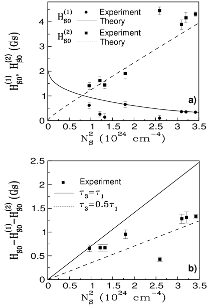
FIG. 4.: Characteristic magnetic fields as a function of the electron density $N_{s}$.
a) – Density dependencies of the Dresselhaus ($H^{(1)}_{SO}$) and Rashba ($H^{(2)}_{SO}$) linear terms are shown by dotted and solid lines, respectively. Calculations were done according to Eq. 57 with $\gamma=24{\ \rm eV\AA^{3}}$ and $\alpha_{0}=7.3{\ \rm\AA^{2}}$. The values of these fields as obtained from best fit with the Sec. II theory are shown by squares (Rashba term) and circles (Dresselhaus term).
b) – The Dresselhaus cubic term $H_{SO}-H^{(1)}_{SO}-H^{(2)}_{SO}$ as a function of $N_{s}$. The lines are calculated using Eq. 57 for $\gamma=24{\ \rm eV\AA^{3}}$. Solid line shows results for an isotropic scattering, $\tau_{1}/\tau_{3}=1$, Dotted line – for $\tau_{1}/\tau_{3}=2$.

In Fig. 4 we show the values of $H^{(1)}_{SO}$ and $H^{(2)}_{SO}$ as a function of $N_{s}^{2}$ for all samples we have studied, as obtained from the fitting of the experimental results by our theory. We also show the theoretical curves for these fields, calculated using Eqs. (5–9) and (57):

$$H^{(1)}_{SO}=\eta_{1}\gamma^{2}N_{s}^{2}\left(\frac{m}{m_{0}}\right)^{2}\left(4\frac{E_{Z}}{E_{F}}-1\right)^{2},$$ (70)

$$H^{(2)}_{SO}=\eta_{2}\alpha_{0}^{2}N_{s}^{2}\left(\frac{m}{m_{0}}\right)^{2}\frac{1}{\kappa^{2}}\left(2\frac{N_{0}}{N_{s}}+1\right)^{2},$$ (71)

where $N_{0}$ is the charge density in the depletion layer, $E_{z}=\hbar^{2}\langle k_{z}^{2}\rangle/2m$ is the kinetic energy of motion in $z$-direction, and

$$\eta_{1}=\frac{\pi^{2}cm_{0}^{2}}{4e\hbar^{3}},\ \eta_{2}=\frac{4\pi^{2}cm_{0}^{2}e^{3}}{\hbar^{3}}.$$ (72)

Here $m_{0}$ is a free electron mass. The calculations are done for $\gamma=24{\ \rm eV\AA^{3}}$ and $\alpha_{0}=7.2{\ \rm\AA^{2}}$. These values allow a good description of the experimental data and are close to those obtained from $\mbox{\boldmath$k$}\cdot\mbox{\boldmath$p$}$ and tight-binding calculations for ${\rm Ga_{0.85}In_{0.15}As}$ (see the Appendix). The ratio $E_{Z}/E_{F}$ is calculated using Fig. 2. When calculating $H^{(2)}_{SO}$, we have assumed that the average field in the well is one half of the maximum field ${\cal E}=4\pi eN_{s}/\kappa$. We have also taken into account the charge in the depletion layer $N_{0}=0.58\cdot 10^{11}{\ \rm cm^{-2}}$. The value of $\alpha_{0}$ was calculated using Eq. (A2). If one takes into account the barriers, using theory of Refs. [28, 29] and the self-consistently calculated wave functions, the value of $\alpha_{0}$ will increase by about 60% for the electron densities in the interval $N_{s}=(1-2)\cdot 10^{12}{\ \rm cm^{-2}}$. This would increase the value of $H^{(2)}_{SO}$ approximately 2.5 times, but such large values of $H^{(2)}_{SO}$ clearly do not agree with the experiment. It is likely that the barrier contribution depends very strongly on their microscopic structure, which may be very different from the abrupt interface model, used in the theory. It is also plausible that the different barrier structure is responsible for the relatively large value of $H^{(2)}_{SO}$ for the sample C1, for which $\alpha_{0}=8.8{\ \rm\AA}$.

It can be shown using the Eq. (5) and data of Fig. 2 that for $N_{s}<N_{s0}=7\cdot 10^{12}{\ \rm cm^{-2}}$ the Dresselhaus term decreases with increasing $N_{s}$, vanishes for $N_{s}=N_{s0}$, and then begins to increase. One can see from Fig. 4 that for $N_{s}>1\cdot 10^{12}{\ \rm cm^{-2}}$ the Rashba term exceeds the Dresselhaus term. Consequently, we denote the larger contribution in Fig. 4 as $H^{(2)}_{SO}$.

TABLE III.: Values of the parameters for GaAs and InAs calculated using the $sp_{3}s^{*}$ model and the results of the $k\cdot p$ model. The parameters of $k\cdot p$ model were taken from Ref. [44], except those marked by asterisk, which were taken from Ref. [46]. Parameters for ${\rm Ga_{0.85}In_{0.15}As}$ were obtained by linear interpolation of the $k\cdot p$ model parameters between GaAs and InAs. The values of $\gamma$ and $\alpha_{0}$ as obtained in these models are also given.

	GaAs		InAs		${\rm Ga_{0.85}In_{0.15}As}$
	$k\cdot p$	$sp_{3}s^{*}$	$k\cdot p$	$sp_{3}s^{*}$	$k\cdot p$	$sp_{3}s^{*}$
$E_{g}$ (eV)	1.519	1.5192	0.42	0.418	1.35	1.354
$\Delta$ (eV)	0.341	0.341	0.38	0.38	0.347	0.347
$E_{g}^{\prime}$ (eV)	2.97	2.98	3.97	3.95	3.12	3.104
$\Delta^{\prime}$ (eV)	0.171	0.159	0.24	0.26	0.181	0.20
$P$ (eV Å)	10.49∗	10.23	9.2∗	9.22	10.29	10.16
$P^{\prime}$ (eV Å)	4.78∗	1.46	0.87∗	1.06	4.20	1.03
$Q$a (eV Å)	-8.16∗	-7.0	-8.33∗	-7.27	-8.18	-7.03
$\frac{m}{m_{0}}$	0.0665	0.066	0.023	0.023	0.06	0.06
$\gamma{\rm\ (eV\AA^{3}})$	27.5	10	26.9	71	27.7	13
$\alpha_{0}{\rm\ (\AA^{2})}$	5.33	5.15	116.74	118.5	7.2	7.05

One can see from Figure 4 that the general character of the density dependence of $H^{(1)}_{SO}$ and $H^{(2)}_{SO}$ agrees with the theory, and their values are close to those calculated using the above values of $\gamma$ and $\alpha_{0}$.

In Fig. 4 b we show a similar density dependence but for the cubic in $k$ Dresselhaus term $H_{SO}-H^{\prime}_{SO}$. The theoretical formula for this field is

$$H_{SO}-H^{\prime}_{SO}=\eta_{1}\gamma^{2}\left(\frac{m}{m_{0}}\right)^{2}N_{s}^{2}\frac{\tau_{3}}{\tau_{1}}.$$ (73)

The top curve corresponds to $\tau_{1}/\tau_{3}=1$ and the bottom one – to $\tau_{1}/\tau_{3}=2$.

In the case of isotropic scattering, which is the case of short range potentials scattering, probabillity $W(\varphi)$ in formula Eq. (12) is angle independent and $\tau_{1}/\tau_{3}=1$. If only small angle scattering is important (that is the case of scattering by the Coulomb potential) then $\tau_{1}/\tau_{3}=9$ (see Eq. (14)). In our case we find $\tau_{1}/\tau_{3}$ to be in the range from 1 to 2. It is probably because scattering in our samples is the mixture of short and long range scattering. The short range scattering is probably due to alloy scattering that is known to be mobility limiting mechanism in GaInAs quantum wells. Long range scattering is most probably due to scattering on the ionized impurities in the $\delta$-doped layer. Role of scattering by the charged impurities in the $\delta$-doped layer was confirmed by observations of charge correlation effects (see Ref. [30]).

V Conclusion

In conclusion, we have presented new experimental studies of positive magnetoconductivity caused by the weak localization in selectively doped GaIn As quantum wells with different carrier densities. The complete interpretation of the observations is obtained in the framework of recently developed comprehensive theory of quantum corrections to conductivity. In this theory, we correctly take into account both linear and cubic in the wave vector terms of the spin splitting Hamiltonian. These terms arise due to the lack of the inversion symmetry of the crystal. We also include the linear splitting terms which appear when the quantum well itself is not symmetric.

It is shown that in the density range where all the above terms are comparable, the new theory allows not only to achieve good agreement with the experiment but, unlike earlier theories, also gives the values for the parameters of the spin splitting which are in agreement with previous optical experiments [9, 12] and theoretical calculations. Therefore, our research answers the question what spin relaxation mechanism dominates for different electron densities and how it should be taken into account to describe the weak localization and antylocalization phenomena in quantum wells

VI Acknowledgments

S. V. Iordanskii and G. E. Pikus thank CNRS and University of Montpellier for invitation and financial support during they stay in France. We would especially thank M. I. Dyakonov and V. I. Perel for helpful advice and illuminating discussions. We would like also thank B. Jusserand, B. Etienne, T. Dietl for useful discussions. The authors acknowledge support by the San Diego Supercomputer Center, where part of the calculations were performed. The research was supported in part by the Soros Foundation (G. E. P.). F. G. P. acknowledges the support by NSF grant DMR993-08011 and by the Center for Quantized Electronic Structures (QUEST) of UCSB. Authors affiliated with the Universite Montpellier acknowledge the support from Schlumberger Industries and Ministere de la Recherche et de la Technologie.

A Spin Splitting in GaAs, InAs, and GaInAs

Below we present results of the calculations of $\alpha_{0}$ and $\gamma$ for GaAs, InAs and ${\rm Ga_{0.85}In_{0.15}As}$ in $\mbox{\boldmath$k$}\cdot\mbox{\boldmath$p$}$ and tight-binding calculations. The tight-binding calculations were done in the 20 band tight-binding model including the spin-orbit coupling[39, 40]. Our calculations of electronic properties use $sp_{3}s^{*}$ tight-binding parameters especially chosen so as to reproduce several features of the fundamental properties of bulk constituents. We state some analytical relations connecting the effective masses and the deformation potentials at the $\Gamma$ point, and the fifteen parameters of the $sp_{3}s^{*}$ 20 band tight-binding model[43]. Using these relations, as well as other relations between the fifteen parameters and $\Gamma$ and $X$ energy values[40], we get a set of parameters which accurately reproduces the effective masses at the $\Gamma$ point, the [001] deformation potential and overall band structure in accordance with reflectivity and photoemission measurements[44].

Such a procedure has been already checked to give a good description of reflectivity data in uniaxially stressed GaAs/${\rm Ga_{0.89}In_{0.11}As}$ superlattices[45]. In this work we use it to obtain InAs and ${\rm Ga_{0.85}In_{0.15}As}$ parameters. Using these parameters, we calculate $\alpha_{0}$ on the basis of Eq. (A2). In order to determine the value of $\gamma$ we calculate the value of the spin splitting as a function of k along (110) direction. It follows a cubic dependence in $k$ from which we extract the values of $\gamma$ given in Table III. The parameters of the $\mbox{\boldmath$k$}\cdot\mbox{\boldmath$p$}$ model were taken from Refs. [44, 46]. The $\mbox{\boldmath$k$}\cdot\mbox{\boldmath$p$}$ parameters for ${\rm Ga_{0.85}In_{0.15}As}$ were obtained by linear interpolation between GaAs and InAs.

In the 3-band $\mbox{\boldmath$k$}\cdot\mbox{\boldmath$p$}$ model one takes into account the states of the conduction band $\Gamma_{1}$ ( $\Gamma_{6}$) with the Bloch function $S$, the valence band $\Gamma_{15\,v}$ ($\Gamma_{8}+\Gamma_{7}$) with functions $X$, $Y$, $Z$, and the higher band $\Gamma_{15\,c}$ ($\Gamma_{8c}+\Gamma_{7c}$) with functions $X^{\prime}$, $Y^{\prime}$, and $Z^{\prime}$. The energies of these states at $k=0$ are: $E_{\Gamma_{6}}=0$, $E_{\Gamma_{8}}=-E_{g}$, $E_{\Gamma_{7}}=-(E_{g}+\Delta)$, $E_{\Gamma_{7c}}=E^{\prime}_{g}$, and $E_{\Gamma_{8c}}=E^{\prime}_{g}+\Delta^{\prime}$. In this model $m_{0}/m$, $\gamma$, and $\alpha_{0}$ are given by the following expressions [9, 47, 48, 49, 50, 28, 51]:

$$\frac{m_{0}}{m} = 1+\frac{2}{3}\frac{m_{0}}{\hbar^{2}}\Biggl{\{}P^{2}\frac{3E_{g}+2\Delta}{E_{g}(E_{g}+\Delta)}+P^{\prime^{2}}\frac{3E_{g}^{\prime}+\Delta^{\prime}}{E^{\prime}_{g}(E_{g}^{\prime}+\Delta^{\prime})}\Biggr{\}},$$ (A1)

$$\gamma = -\frac{4}{3}\frac{PP^{\prime}Q}{E_{g}(E_{g}^{\prime}+\Delta^{\prime})}\left(\frac{\Delta}{E_{g}+\Delta}+\frac{\Delta^{\prime}}{E_{g}^{\prime}}\right),$$ (A2)

$$\alpha_{0} = \frac{1}{3}\Biggl{\{}P^{2}\left[E_{g}^{-2}-(E_{g}+\Delta)^{-2}\right]-$$ (A4)

$$P^{\prime^{2}}\left[{E_{g}^{\prime}}^{-2}-(E_{g}^{\prime}+\Delta^{\prime})^{-2}\right]\Biggl{\}},$$

where $P=i\hbar/m_{0}\,\langle S|p_{z}|Z\rangle$, $P^{\prime}=i\hbar/m_{0}\,\langle S|p_{z}|Z^{\prime}\rangle$, and $Q=i\hbar/m_{0}\,\langle X|p_{y}|Z^{\prime}\rangle$ are the interband matrix elements, $m_{0}$ is the free electron mass, $\mbox{\boldmath$p$}=-i\hbar\nabla$. Here we do not take into account the contribution into $\gamma$ and $\alpha_{0}$ which arises from spin-orbit mixing of the states $\Gamma_{15\,v}$ and $\Gamma_{15\,c}$.

The values of $\gamma$ obtained for GaAs from tight-binding calculations are usually smaller then those given by the $k\cdot p$ model (see Table III). For example, in Ref. [41] the tight-binding calculations give the value $2\gamma=17.8{\ \rm eV\AA^{3}}$. In the later work Ref. [42] for the same parameter $2\gamma$ (this time called $\gamma$) authors obtain the value $17{\ \rm eV\AA^{3}}$. Calculated values of $\gamma$ should be compared to the experimental values $24{\ \rm eV\AA^{3}}$ for bulk GaAs[9] and to the recently obtained value for GaAs/GaAlAs quantum wells[12] $16.5\pm 3{\ \rm eV\AA^{3}}$.

REFERENCES

- [1] Permanent address: Unipress PAN Sokolowska 92, Warsaw, Poland.
- [2] Permanent address: Physics Department of Warsaw University 02689, Warsaw, Poland.
- [3] E. Abrahams, P. Anderson, D. Licciardello, and T. Ramakrishnan, Phys. Rev. Lett. 42, 673 (1979).
- [4] L. Gorkov, A. Larkin, and D. Khmelnitskii, Pisma Zh. Eksp. Teor. Fiz. 30, 248 (1979) [JETP Letters 30, 228 (1979)].
- [5] Note that similar effects were also observed and described in optics (see review Yu. N. Barabanenkiv, Uspehi Fiz. Nauk. 117, 49 (1975) [Sov. Phys. - Uspekhi 18, 673 (1975)]. Moreover, an additive contribution to the backscattering due to interference of excitonic waves was considered in G. L. Bir, E. L. Ivchenko, and G. E. Pikus, Izv. Acad. Sci. SSSR (ser Fiz) 40, 1866 (1976) [Bull. Acad. Sci. USSR Phys. Ser. 40, 81 (1976)]; E. L. Ivchenko, G. E. Pikus, B. S. Razbirin, and A. I. Starukhin, Zh. Eksper. Teor. Fiz. 72, 2230 (1977) [Sov. Phys. JETP 45, 1172 (1977)].
- [6] B. Altshuler, D. Khmelnitskii, A. Larkin and P. Lee, Phys. Rev. B 22, 5142 (1980).
- [7] S. Hikami, A. Larkin, and Y. Nagaoka. Progr. Theor. Phys. 63, 707 (1980).
- [8] B. L. Altshuler, A. G. Aronov, A. I. Larkin, and D. E. Khmelnitskii, JETP 54, 411 (1981) (JETP 81, 788 (1981)).
- [9] G. E. Pikus and A. Titkov, in “Optical orientation”, ed. by F. Mayer and B. Zakharchenya, North Holland, Amsterdam (1984).
- [10] G. Dresselhaus, Phys. Rev. 100, 580 (1955).
- [11] Yu. L. Bychkov and E. I. Rashba, J. Phys. C 17, 6093 (1984).
- [12] B. Jusserand, D. Richards, G. Allan, C. Priester, and B. Etienne, Phys. Rev. B. 51, 4707 (1995).
- [13] This correlation is also the cause of various photogalvanic effects in gyrotropic crystals and in low-dimensional structures. The photocurrent due to correlation of angular momentum and momentum of holes was studied in E. L. Ivchenko and G. E. Pikus, Zh. Eksper. Teor. Fiz. Pisma 27, 640 (1978) [JETP Lett. 27, 604 (1978)]. For review, bibliography, and effects connected to the linear in momentum spin Hamiltonian of the conduction electrons see E. L. Ivchenko, Yu. B. Lyanda-Geller, and G. E. Pikus, JETP 71, 550 (1990) (ZhETF 98, 989 (1990)). A. G. Aronov, Yu. B. Lyanda-Geller, and G. E. Pikus, JETP 73, 573 (1991) (ZhETF 100, 973 (1991)).
- [14] H. Mathur and A. D. Stone, Phys. Rev. Lett. 68, 2964 (1992).
- [15] A. G. Aronov and Yu. B. Lyanda-Geller. Preprint Univ. of Karlsruhe. 1993; the consise summary of these results and ballistic vector-potential effects can be found in Proc. 22 Int. Conf. Phys. Semicond, Vancouver 1994, Ed. by D. J. Lockwood, World Scientific, Singapore, 1995, p. 1995.
- [16] Yu. B. Lyanda-Geller and A. D. Mirlin. Phys. Rev. Lett. 72, 1894 (1994).
- [17] S. V. Iordanskii, Yu. B. Lyanda-Geller, and G. E. Pikus, JETP Letters 60, 206 (1994) (Pisma v JETP 60, 199 (1994)).
- [18] F. G. Pikus and G. E. Pikus, Phys. Rev. B. 51, 16928 (1995).
- [19] Yu. B. Lyanda-Geller, In Proc. XI International Conf. on Electronic Properties of systems, Nottingham, 1995, to be published in Surface Science.
- [20] D. A. Poole, M. Peper, and A. Hugness, J. Phys. C 15, L1137 (1982), J. Phys. C 17, 6039 (1984).
- [21] V. A. Beresovetz, I. I. Farbstein, and A. L. Shelankov, JETP Lett. 39, 74 (1984) (Pisma v JETP 39, 64 (1984)).
- [22] Y. Kawaguchi, I. Takayanagi, and S. Kawaji, J. Phys. Sos. Jpn. 56, 1293 (1987).
- [23] P. D. Dresselhaus, C. M. M. Papavassiliou, R. G. Wheeler, and R. N. Sacks, Phys. Rev. Lett. 68, 106 (1992).
- [24] J. E. Hansen, R. Taboryski, and P. E. Lindelof, Phys. Rev. B 47, 16040 (1993).
- [25] G. L. Chen, J. Han, T. T. Huang, S. Datta, and D. B. Janes, Phys. Rev. B 47, 4084 (1993).
- [26] W. Knap, C. Skierbiszewski, G. E. Pikus, E. Litwin-Staszewska, S. V. Iordanskii, F. Kobbi, A. Zduniak, J. L. Robert, V. Mosser, and K. Zekentes, in Proc. 22 Int. Conf. Phys. Semicond, Vancouver 1994, Ed. by D. J. Lockwood, World Scientific, Singapore, 1995, p. 835.
- [27] M. I. Dyakonov and Y. Yu. Kachorovskii, Sov. Phys. Semicond. 20, 110 (1986).
- [28] L. G. Gerchikov and A. W. Subashiev, Sov. Phys. Semicond. 26, 73 (1992) (Fiz. Techn. Poluprov. 26, 131 (1992)).
- [29] G. E. Pikus and U. Rössler, unpublished.
- [30] E. Litwin-Staszewska, F. Kobbi, M. Kamal-Saadi, D. Dur, C. Skierbiszewski, H. Sibari, K. Zekentes, V. Mosser, A. Raymond, W. Knap, and J. L. Robert, Solid state Electron. 37, 665 (1994).
- [31] F. Stern, Phys. Rev. B 5, 4891 (1972).
- [32] A. B. Fowler and F. Stern, Rev. Mod. Phys. 54, 437 (1982).
- [33] W. Knap, D. Dur and A. Raymond, C. Meny and J. Leotin, S. Huant, B. Etienne, Rev. Sci. Instrum., 63, 3293 (1992).
- [34] S. Chakravarty and A. Schmid, Physics Report 140, 193 (1986).
- [35] A. Kawabata, J. Phys. Soc. Japan, 49, 628 (1980); it ibid 53, 3540 (1984).
- [36] M. I. Dyakonov, Solid State Commun., 92, 711 (1994).
- [37] A. Zduniak, M. I. Dyakonov, and W. Knap, in Proceedings of International Conference on Semiconductor Heteroepitaxy, Montpellier (1995), in print.
- [38] P. T. Boggs et. al, NIST preprint NISTIR 92-4834.
- [39] P. Vögl, H. P. Hjalmarson, and J. D. Dow, J. Chem. Solids, 44, 365 (1983).
- [40] A. Kobayashi, O. F. Sankey and J. D. Dow, Phys. Rev. B 25, 6367 (1982).
- [41] P. V. Santos and M. Cardona, Phys. Rev. Lett. 72, 3 (1994).
- [42] P. V. Santos, M. Willatzen, M. Cardona, and A. Santarero, Phys. Rev. B 51, 121 (1995).
- [43] D. Bertho and C. Jouanin. Private communication.
- [44] Numerical data and functional Relationships in Science and Technology, edited by O. Madelung, Landolt-Börnstein, New Series, Group III, Vol. 17, Parts a and b, Springer-Verlag, Berlin 1982; Vol. 22, Pt. a, Springer-Verlag, Berlin 1987.
- [45] P. Boring, J. M. Jancu, B. Gil, D. Bertho, C. Jouanin and K. J. Moore, Phys Rev. B 46, 4764, (1992).
- [46] C. Hermann and C. Weisbuch Phys. Rev. B 15, 823 (1977).
- [47] M. Cardona, N. E. Christensen, and G. Fasol, Phys. Rev. B 38, 1806 (1988).
- [48] E. L. Ivchenko and G. E. Pikus, “Superlattices and other Heterostructures: Symmetry and Optical Phenomena”. Springer Series in Solid-State Sciences, 110, Springer-Verlag, Berlin, 1995.
- [49] F. Malcher, G. Lommer, and U. Rössler, Superlattices and Microstructures, 2, 278 (1986); Phys. Rev. Lett. 60, 278 (1988).
- [50] U. Rössler, F. Malcher, and G. Lommer, Springer Series in Solid State Sciences 87, ”High Magnetic Fields in Semiconductors”, Physics II, Ed. by G. Landwehr, Springer-Verlag, Berlin Heidelberg, 1989, p. 376.
- [51] In Eq. (A2) we have corrected some misprints made in the cited papers.