COMPLETE WETTING IN THE THREE-DIMENSIONAL TRANSVERSE ISING MODEL

Abstract

We consider a three-dimensional Ising model in a transverse magnetic field, $h$ and a bulk field $H$. An interface is introduced by an appropriate choice of boundary conditions. At the point $(H=0,h=0)$ spin configurations corresponding to different positions of the interface are degenerate. By studying the phase diagram near this multiphase point using quantum-mechanical perturbation theory we show that that quantum fluctuations, controlled by $h$, split the multiphase degeneracy giving rise to an infinite sequence of layering transitions.

I INTRODUCTION

There is a considerable body of literature discussing the way in which interfaces depin from surfaces[[1]]. Of particular interest to us here is the situation below the roughening transition when the interface is smooth and can depin from the surface through a series of first-order layering transitions.

This possibility was first pointed out by De Oliveira and Griffiths[[2]] for a model in which the layering is driven by the competition between a long-range bulk interaction and a surface field. Here the layering transitions exist even at zero temperature. Later Duxbury and Yeomans[[3]] showed that, if the position of the interface relative to the surface was degenerate at zero temperature, the degeneracy could be split by thermal fluctuations giving an infinite series of layering transitions at finite temperatures. The stable interface position is determined as a balance between the binding effect of a bulk field and the entropic advantage for the interface lying further from the surface.

The transverse Ising model [[4]] was first introduced by de Gennes [[5]] in connection with ferro-electric materials. Recently Henkel et. al.[[6]] have discussed the behaviour of a domain wall in this system. The interesting questions concern the effect of quantum fluctuations, mediated by the transverse field, on the behaviour of the interface. Their work considers one dimension where the interface is rough. Very different behaviour is likely for a smooth interface. Therefore in this paper we consider the behaviour of the three-dimensional transverse Ising model below the roughening temperature. We find that a zero-temperature multiphase point can be split by quantum fluctuations and that, for a non-zero transverse field, there are an infinite number of stable positions for the interface as a bulk field passes through zero.

The next section of the paper defines the model and gives a qualitative discussion of its properties and our approach. Quantitative details of the calculation, which is based on quantum mechanical perturbation theory, are given in Sec. III. Our conclusions are summarized in Sec. IV.

II QUALITATIVE REMARKS

The Hamiltonian of the three-dimensional transverse Ising model we shall consider is

$${\cal H}= - J_{0}\sum_{i=1,L}\sum_{\langle j,j^{\prime}\rangle}S_{z}(i,j)S_{z}(i,j^{\prime})-j\sum_{i=0,L}\sum_{j}S_{z}(i,j)S_{z}(i+1,j)$$ (1)

$$- \sum_{i=1,L}\sum_{j}\biggl{[}hS_{x}(i,j)+HS_{z}(i,j)\biggr{]}-K\sum_{j}\biggl{(}S_{z}(0,j)-S_{z}(L+1,j)\biggr{)}\ ,$$ (2)

where $i$ labels two-dimensional planes and $\langle j,j^{\prime}\rangle$ nearest neighbours within a plane. The parameter $K\rightarrow\infty$ is used to impose appropriate boundary conditions, namely to fix the spins at the surface ($i=0$) to be up and those in the last layer ($i=L+1$) to be down. These boundary conditions will create a domain wall, or interface, in the system separating layers of up and down spins (see Fig. 1). Our aim is to construct the phase diagram which gives the position, $k$, of the interface (defined as in Fig. 2a.) as a function of the uniform field $H$ and the transverse field $h$. We shall consider the limit $L\rightarrow\infty$ and zero temperature where the interface is flat.

As a first step in understanding the phase diagram we consider the situation for $h=0$. In this case it is clear that for positive $H$, $k=\infty$ whereas for negative $H$, $k=0$. We shall call these phases, which are illustrated in Fig. 2, R and L respectively. For $H$=0 the energy is independent of $k$, so that all interface positions are degenerate. It is known that such a degeneracy can be lifted by either thermal fluctuations[[7]] or by quantum fluctuations[[8]]. In more general contexts this removal of degeneracy has been referred to as ground state selection[[9]] following the work of Villain and Gordon[[11]] and Shender[[10]]. Here we will consider the effect of quantum fluctuations.

There are two possibilities: in the first, quantum fluctuations due to nonzero $h$ cause the transition from L to R to be discontinuous with no intermediate states; in the second this transition occurs through a sequence of intermediate states in which $k$ increases monotonically. This sequence can be finite, so that there is a first-order transition from a state with $k=k_{\rm max}$ to R, or it can be infinite. In general, one expects the first possibility when the effective interaction between the surface and the interface is attractive and the second when this effective interaction is repulsive. Our results indicate that quantum effects give rise to the second possibility and that the sequence of layering transitions is probably an infinite one. It is easy to see that even when $h$ is nonzero, the R phase is stable whenever $H$ is positive. As we will show, the stability of the L phase requires that $H<-Ch^{2}j/J_{0}^{2}$, where $C$ is a constant.

To determine the interface position we must calculate the ground state energy as a function of $H$. To do this we assume perfectly flat interfaces and apply perturbation theory to calculate the energy of the state when the interface is at position $k$. If we were dealing with a finite system, then perturbation theory would introduce coupling in finite order between states when the interface is at different positions. However, this tunneling effect disappears in the thermodynamic limit. Our calculations are valid for $h\ll J$. We also impose the condition $j\ll J_{0}$, although as long as we remain in the regime where the interfaces are flat, this restriction is probably inessential.

The energy per layer spin $e(k)$ of the state when the interface is at position $k$ can be written

$$e(k)=e_{0}(H)-kH+E_{k}(H)\ ,$$ (3)

where $e_{0}(H)$ is the energy per layer spin for the $k=0$ phase. The most important dependence on $H$ is in the term $-kH$. $H$ also contributes to the energy denominators that appear in perturbation theory, which are typically of the form $2J_{0}+j+H$. However perturbative contributions to $E_{k}(H)$, when expanded in powers of $H$, lead to corrections which are of relative order $H/J_{0}$ or smaller. But since we will only be interested in $H$ in the range $-Ch^{2}/J_{0}<H<0$, these corrections are smaller than of relative order $(h^{2}/J_{0}^{2})\ll 1$, which we may ignore. Therefore, in Eq. (3), we may evaluate $E_{k}(H)$ at $H=0$. We shall find that $E_{k}$ is a positive and decreasing function of $k$. This result leads to an infinite sequence of phase transitions. The critical field separating the phase $k$ from $k+1$ is given by

$$-H_{k}^{*}=E_{k}-E_{k+1}\equiv\Delta E_{k}\ ,$$ (4)

where, as argued above, the leading order calculation of $E_{k}$ can be obtained for $H=0$.

III CALCULATION OF $\Delta E_{k}$

From Eq. (4) it is clear that we only need to keep track of terms in the ground-state energy which depend on $k$. In other words we need to ascertain how the corrections to the ground–state energy which are perturbative in $h$ depend on the location of the interface. For convenience we now transform to occupation number operators. For spins that are up (down) we write $S_{z}(i,j)=1/2-n_{i,j}$ ($S_{z}(i,j)=-1/2+n_{i,j}$). Also $S_{x}(i,j)=(a^{\dagger}_{i,j}+a_{i,j})/2$, where the operator $a^{\dagger}_{i,j}$ ($a_{i,j}$) creates (destroys) a Bose excitation at site $i$ in the $j$th layer and $n_{i,j}=a_{i,j}a_{i,j}^{\dagger}$. Strictly speaking we should not allow more than one excitation to exist on a single site. To enforce this restriction we include a term of the form $\Lambda\sum_{i,j}a_{i,j}^{\dagger}a_{i,j}^{\dagger}a_{i,j}a_{i,j}$, where $\Lambda\rightarrow\infty$. Normally, it is difficult to take full account of such a hard-core interaction. As we will see, we accommodate this constraint by never involving matrix elements connecting to a state in which there is more than one excitation at any site. Therefore, setting $H=0$, we are lead to the following bosonic Hamiltonian, when the interface is at position $k$:

$${\cal H}_{B}= E_{0}+\sum_{i=1}^{\infty}\sum_{j}\biggl{(}2J_{0}n_{i,j}-(h/2)[a^{\dagger}_{i,j}+a_{i,j}]\biggr{)}-\sum_{i=1}^{\infty}\sum_{\langle j,j^{\prime}\rangle}J_{0}n_{i,j}n_{i,j^{\prime}}+\Lambda\sum_{i=1}^{\infty}\sum_{j}a_{i,j}^{\dagger}a_{i,j}^{\dagger}a_{i,j}a_{i,j}$$ (6)

$$-j\sum_{i=0}^{\infty}\sum_{j}[-(1/2)(n_{i,j}+n_{i+1,j})+n_{i,j}n_{i+1,j}]+j\sum_{j}[-n_{k,j}-n_{k+1,j}+2n_{k,j}n_{k+1,j}]\ ,$$

where $E_{0}$ is the unperturbed energy of the $k=0$ phase, $\Lambda\rightarrow\infty$, and for $K\rightarrow\infty$, we may set $n_{0,j}=0$. We write this Hamiltonian as

$${\cal H}_{B}=E_{0}+{\cal H}_{0}+V_{1}+V_{2}+V_{3}+V_{4}\ ,$$ (7)

where

$${\cal H}_{0}=\Delta\sum_{i}\sum_{j}n_{i,j}\ ,$$ (8)

with $\Delta=2J_{0}+j$,

$$V_{1}=-\sum_{i}\sum_{j}j_{i,i+1}n_{i,j}n_{i+1,j}-J_{0}\sum_{i}\sum_{\langle j,j^{\prime}\rangle}n_{i,j}n_{i,j^{\prime}}$$ (9)

$$V_{2}=-(h/2)\sum_{i}\sum_{j}[a_{i,j}^{\dagger}+a_{i,j}]\ ,$$ (10)

$$V_{3}=-j\sum_{j}(n_{k,j}+n_{k+1,j})\ ,$$ (11)

where

$$j_{i,i+1}=\left\{\begin{array}[]{ll}j&\mbox{for }i\not=k\\ -j&\mbox{for }i=k\end{array}\right.$$ (12)

and (with $\Lambda\rightarrow\infty$)

$$V_{4}=\Lambda\sum_{i}\sum_{j}a_{i,j}^{\dagger}a_{i,j}^{\dagger}a_{i,j}a_{i,j}\ .$$ (13)

We now consider how the perturbative contributions to the energy depend on the various coupling constants. To carry out this discussion it is convenient to introduce a diagrammatic representation of the contributions to the perturbation expansion. Each term of $V_{1}$ proportional to $j_{rs}n_{r}n_{s}$, where $r$ (and similarly $s$) denotes a position label of the form $i,j$, is represented by a line joining the two interacting sites $r$ and $s$ and $j_{rs}=J_{0}$ or $j_{rs}=j$ depending on whether sites $r$ and $s$ are in the same plane or are in adjacent planes. The perturbation in $V_{2}$ proportional to $a_{r}$ ($a_{r}^{\dagger}$) is represented by a minus (plus) sign at the site $r$. However, for simplicity, since each site involved with any of the preceding interactions must be excited (i. e. must have both a ”+” and a ”-” associated with it), we have not explicitly shown ”+”’s and ”-”’s in Fig. 3. The term in the perturbation $V_{3}$ proportional to $n_{k,j}$ ($n_{k+1,j}$) is represented by a circle attached to the site $k,j$ ($k+1,j$). Any term in perturbation theory which does not involve $V_{4}$ can be constructed from these elements. Some simple examples are shown in Fig. 3.

We now define what we mean by connected terms. Any term which involves only a single site is connected. Terms which involve more than one site are connected only if all such sites are connected with respect to lines representing terms of $V_{1}$. If this is not the case, the term will be called disconnected. Thus diagrams (a) and (d) of Fig. 3 are disconnected.

We now establish that contributions from disconnected configurations of lines vanish.

Consider a disconnected diagram $\Gamma$ which consists of two disjoint components, $\Gamma_{A}$ and $\Gamma_{B}$. The contribution of of this diagram is unchanged if we were to treat perturbatively the system $S(\Gamma_{A}+\Gamma_{B})$ in which all coupling constants $j_{rs}$ not in $\Gamma_{A}$ or $\Gamma_{B}$ are set to zero. But because $\Gamma_{A}$ and $\Gamma_{B}$ are disjoint systems, we have $E(\Gamma_{A}+\Gamma_{B})=E(\Gamma_{A})+E(\Gamma_{B})$. This result indicates that there are NO disconnected terms in the ground state energy which involve simultaneously an exchange constant from one component $\Gamma_{A}$ and an exchange constant from the other component $\Gamma_{B}$. Thus disconnected diagrams can be omitted from further consideration.

To evaluate $\Delta E_{k}$ it is apparent from the form of Eq. (3) that we only need to keep contributions which appear when the interface is at position $k+1$ but NOT when it is at position $k$. Note that if the diagram does not involve the interface potential $V_{3}$, it has no dependence on position and will make equal contributions in the two cases. So $\Delta E_{k}$ has contributions from diagrams which both a) involve $V_{3}$, the interface potential, and b) can occur when the interface is at position $k+1$ but not at position $k$. Such a connected diagram must involve sites in rows 1, 2, … $k+1$. This can be done with diagrams involving $k$ or more lines. As we will see in a moment, the dominant contribution involves the least number of lines. To take the least number of lines, means that we take $k$ lines representing $j$ and no lines representing $J_{0}$. Thus the dominant diagrams are linear chain diagrams, and we may therefore consider a Hamiltonian in which the index $j$ in Eqs. (8)–(13) is omitted. We illustrate the diagrams with the minimum number of lines which contribute to $\Delta E_{k}$ for $k=0$ and $k=1$ in Figs. 4 and 5 respectively.

To check that it is indeed the linear chain diagrams which give the lowest order contribution to $\Delta E_{k}$ it is necessary to give a more detailed analysis of the contribution of a diagram involving, say, $p$ different lines representing $V_{1}$ and, as we explained, necessarily involving at least one interface potential term $V_{3}$. Note that both these perturbations, $V_{1}$ and $V_{3}$, involve occupation numbers $n_{r}$, which vanish when there is no excitation at site $r$. For every site $r$ involved in a $V_{1}$ or $V_{3}$ interaction, it is necessary to create an excitation so that $n_{r}$ can be evaluated in a virtual state in which $n_{r}=1$. Subsequently, in order to get back into the ground state we must destroy the excitation on the site $r$. Thus in all a diagram involving $p$ different lines will involve $p+1$ sites and therefore give rise to a perturbative contribution to the energy which is of order $\delta_{p}E$, where

$$\delta_{p}E=h^{(2p+2)}j^{p_{1}}J_{0}^{p_{2}}(j/\Delta)/\Delta^{2p+1+p_{1}+p_{2}}\ ,$$ (14)

where of the $p$ lines, $p_{1}$ are associated with $j$ and $p_{2}$ with $J_{0}$ [see Eq. (9)]. In writing this equation we included the factor $(j/\Delta)$ to take account of the necessary factor of $V_{3}$. At this point, it is clear that to have a diagram which occurs for position $k+1$ but not for $k$ it is best to invoke a linear diagram, and not one which reaches more than one row perpendicular to the interface. Unnecessary factors of $J_{0}$ in $V_{1}$ will give rise to additional factor of $J_{0}h^{2}/\Delta^{3}\ll 1$. So, we conclude that to leading order

$$\Delta E_{k}=C_{k}J_{0}^{2}[jh_{0}^{2}/J_{0}^{3}]^{k+1}\ ,$$ (15)

where $C_{k}$ is a constant which must be determined by an explicit calculation and to leading order we set $\Delta=2J_{0}$.

Now let us carry out a detailed calculation for the simplest case, namely for $k=0$. From Fig. 4 we obtain

$$\Delta E_{0}=-E(A1)\ ,$$ (16)

where $E(A1)$ is the contribution to the energy in diagram $A1$ of Fig. 4. Thus[[12]]

$$\Delta E_{0} = -\langle 0|V_{2}{1\over{\cal E}}V_{3}{1\over{\cal E}}V_{2}|0\rangle$$ (17)

$$= -\langle 0|(-h/2)a_{1}{1\over{\cal E}}(-ja_{1}^{\dagger}a_{1}){1\over{\cal E}}(-h/2)a_{1}^{\dagger}|0\rangle$$ (18)

$$= (h^{2}/4)(j/\Delta^{2})=jh^{2}/(16J_{0}^{2})\ .$$ (19)

Here and below the excitation energies $\cal E$ will be $-r\Delta=-2rJ_{0}$, where $r$ is the number of excitations in the virtual state.

Next we calculate $\Delta E_{1}=-E(E2)$ from diagram $E2$ of Fig. 5. Here we have to sum over the different orderings of the perturbations.

$$\Delta E_{1}=$$ (24)

$$-\langle 0|\biggl{[}(-h/2)a_{1}{1\over{\cal E}}(-h/2)a_{2}+(-h/2)a_{2}{1\over{\cal E}}(-h/2)a_{1}\biggr{]}{1\over{\cal E}}\biggl{[}(-jn_{1}n_{2}){1\over{\cal E}}(-jn_{2})+(-jn_{2}){1\over{\cal E}}(-jn_{1}n_{2})\biggr{]}$$

$$\ \ \times{1\over{\cal E}}\biggl{[}(-h/2)a_{1}^{\dagger}{1\over{\cal E}}(-h/2)a_{2}^{\dagger}+(-h/2)a_{2}^{\dagger}{1\over{\cal E}}(-h/2)a_{1}^{\dagger}\biggr{]}|0\rangle$$

$$\ \ -\langle 0|\biggl{[}(-h/2)a_{1}{1\over{\cal E}}(-h/2)a_{2}+(-h/2)a_{2}{1\over{\cal E}}(-h/2)a_{1}\biggr{]}{1\over{\cal E}}(-jn_{1}n_{2}){1\over{\cal E}}(-h/2)a_{1}^{\dagger}{1\over{\cal E}}(-jn_{2}){1\over{\cal E}}(-h/2)a_{2}^{\dagger}|0\rangle$$

$$\ \ -\langle 0|(-h/2)a_{2}{1\over{\cal E}}(-jn_{2}){1\over{\cal E}}(-h/2)a_{1}{1\over{\cal E}}(-jn_{1}n_{2}){1\over{\cal E}}\biggl{[}(-h/2)a_{1}^{\dagger}{1\over{\cal E}}(-h/2)a_{2}^{\dagger}+(-h/2)a_{2}^{\dagger}{1\over{\cal E}}(-h/2)a_{1}^{\dagger}\biggr{]}|0\rangle.$$

When simplified this yields

$$\Delta E_{1}=2(h/2)^{4}j^{2}/\Delta^{5}=(1/256)j^{2}h^{4}/J_{0}^{5}\ .$$ (26)

This calculation is hard to extend to $\Delta E_{k}$ for larger $k$ using naive perturbation theory. We need a more powerful formalism, namely Matsubara diagrams[[13]]. In this formalism one has diagrams constructed from the following elements. The perturbations $V_{1}$, $V_{2}$, and $V_{3}$ are represented by vertices as shown in Fig. 6. Each such vertex carries the appropriate factor ($(-h/2)$, $-j\delta_{r,k}$, and $-j$, respectively, where $\delta_{r,k}$ is the Kronecker delta. Also note that at leading order $j_{i,i+1}=j$, because we never invoke the term $j_{k,k+1}$.). Lines labeled with the same index are joined and a sum is taken over all topologically inequivalent connected diagrams. Each line represents a Green’s function $(z_{\nu}-\Delta)^{-1}$. All the indices are summed over. The $z$’s are summed over the Matsubara frequencies $z_{\nu}=2\nu\pi i/(k_{B}T)$ where $\nu$ runs over all integers positive and negative. One enforces conservation of $z$, that is for each vertex the sum of all incoming $z$’s minus the sum of all outgoing $z$’s must equal zero. For the present case, this conservation law mean that at any vertex which has only one line entering or leaving the corresponding $z$ must be zero. One can quickly see that the $z$’s for all lines have to be zero. So, in fact, there is no sum over $z$ to be done. (Such sums normally lead to the Bose occupation number factors.)

From Fig. 7 we see that

$$\Delta E_{0}=-E_{a}\ ,$$ (27)

where $E_{a}$ is the energy from diagram (a) of Fig. 7. (A similar notation for the other diagrams is used below.) Thus

$$\Delta E_{0}=-(-h/2)(-j)(-h/2)(-\Delta)^{-2}=h^{2}j/(4\Delta^{2})=h^{2}j/(16J_{0}^{2})\ ,$$ (28)

as before. To obtain this result, note that diagram (a) has two filled circle vertices (each carrying a factor $-h/2$), one triangle (carrying a factor $-j$), and two lines, each of which carries a factor $(z-E_{i})^{-1}=\Delta^{-1}$. Also from Fig. 7 we have

$$\Delta E_{1}=-(E_{b}+E_{c})=-2E_{b}\ .$$ (29)

Since diagram (b) has four $h$ vertices, two $j$ vertices, and five lines, we have that

$$\Delta E_{1}=-2(-h/2)^{4}(-j)(-j)(-\Delta)^{-5}=h^{4}j^{2}/(8\Delta^{5})=h^{4}j^{2}/(256J_{0}^{5})\ .$$ (30)

Finally, from Fig. 7 we have

$$\Delta E_{2}=-(E_{d}+E_{e}+E_{f}+E_{g})=-4E_{d}\ .$$ (31)

Since diagram (d) has six $h$ vertices, three $j$ vertices, and eight lines

$$\Delta E_{2}=-4(-h/2)^{6}(-j)(-j)^{2}(-\Delta)^{-8}=h^{6}j^{3}/(16\Delta^{8})=h^{6}j^{3}/(4096J_{0}^{8})\ .$$ (32)

Evidently, the general result is

$$\Delta E_{k}=J_{0}(jh^{2}/16J_{0}^{3})^{k+1}\ .$$ (33)

IV CONCLUSIONS

Equation (33) indicates that the boundary between phases with $k=p$ and $k=p+1$ is given to leading order by $H_{p}^{*}=-J_{0}(jh^{2}/16J_{0}^{3})^{p+1}$. The resulting phase diagram is shown schematically in Fig. 8.

The analysis presented above was based on retaining only the leading-order (in $h/J_{0}$ and $j/J_{0}$) term in the surface–interface interaction. Although we cannot rule out the possibility that the neglected higher-order interactions could become dominant for very large $k$ (for fixed $h$ and $J_{0}$), we do not expect to observe any qualitative corrections to the phase diagram in this limit. This is because there are no competing interactions which would make correlation functions oscillatory at large distance and therefore it seems implausible that the positive sign of $\Delta E_{p}$ can be changed by the neglected higher-order terms[[14]].

To summarize we have shown that quantum fluctuations can stabilize an infinite sequence of layering transitions in a three-dimensional transverse Ising model.

FIG. 1.: Schematic representation of the model introduced in Eq. (1). The leftmost plane is labeled $i=0$ and the rightmost $i=L+1$. The surface field $K$ is not shown.

FIG. 2.: a) Configuration of the spins when the interface is at position $k$. Layer 0 is constrained to be up and the layer at infinity is constrained to be down. In panels (b) and (c) we have represented the configurations R and L.

FIG. 3.: Representation of perturbative contributions to the ground state energy. The dashed line corresponds to the location of the interface. (a) A contribution which cannot occur. (b) A term in which a given $j$ is taken to second order. (c) The contribution to lowest order in $j$ which involves four sites. (d),(e),(f) Terms which involved factors of $h^{2}$. (f) A term which involves the $J_{0}$ interaction.

FIG. 4.: Perturbative contributions to the ground-state energy used to evaluate $\Delta E_{0}=E_{0}-E_{1}$. Panel A0 corresponds to the case when the interface is at $k=0$; panels A1 and B1 to the case $k=1$.

FIG. 5.: Perturbative contributions to the ground-state energy used to evaluate $\Delta E_{1}=E_{1}-E_{2}$. Panels A1 – D1 are for the case when the interface is at $k=1$. Panels A2 – E2 correspond to $k=2$. The dashed line represents the position of the interface. Contributions from diagrams A1, B1, C1, and D1 are equal to those from diagrams A2, B2, C2, and D2, respectively. So $\Delta E_{1}$ is determined by E2.

FIG. 6.: Vertices for Matsubara diagrams: (a) transverse field vertex $-(h/2)(a_{m}^{\dagger})$ (top) and $-(h/2)a_{m}$ (bottom); (b) $-j\delta_{r,k}a_{r}^{\dagger}a_{r}$; (c) $-jn_{j}n_{j+1}=ja_{j}^{\dagger}a_{j+1}^{\dagger}a_{j+1}a_{j}$.

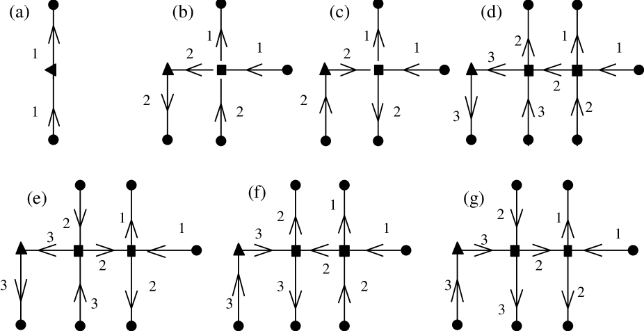
FIG. 7.: Matsubara diagrams. The vertices are explained in the preceding figure. The lines are labeled by an index $i$ to represent the Green’s function $(z-\Delta)^{-1}$. This calculation is for a linear system with sites labeled 1, 2, …. These diagram give $-\Delta E_{m}$ following the reasoning of Figs. 4 and 5. Diagram (a) is for $m=0$, diagrams (b) and (c) are for $m=1$ and diagrams (d)–(g) are for $m=2$. No new topology is obtained by reversing the direction of the line labeled ”1”. However, one may independently reverse the direction of all other lines giving rise to a degeneracy $2^{m}$.

FIG. 8.: Schematic representation of the phase diagram for interface unbinding transitions in the transverse Ising model.

- [1] S. Dietrich in Phase Transitions and Critical Phenomena, edited by C. Domb and J. L. Lebowitz (Academic, New York, 1988), Vol. 12. p. 1 ; R. Pandit, M. Schick and M. Worthis, Phys. Rev. B 26, 5112 (1982)
- [2] M. J. De Oliveira and R. B. Griffiths, Surf. Sci. 71, 687 (1978).
- [3] P. M. Duxbury and J. M. Yeomans, J. Phys. A 18, L983 (1985).
- [4] R. B. Stinchcombe, J. Phys. C 6, 2459 (1973).
- [5] P.G. de Gennes, Solid St. Commun. 1, 132 (1963).
- [6] M. Henkel, A.B. Harris and M. Cieplak, Phys. Rev. B52, 4371 (1995).
- [7] W. Selke, in Phase Transitions and Critical Phenomena, edited by C. Domb and J. L. Lebowitz (Academic, New York, 1992), Vol. 15.
- [8] A.B. Harris, C. Micheletti and J.M. Yeomans, Phys. Rev. Lett. 74, 3045 (1995); Phys. Rev. B52, 6684 (1995).
- [9] C. L. Henley, Phys. Rev. Lett. 62, 2056 (1989).
- [10] E. F. Shender, Sov. Phys. JETP 56, 178 (1982).
- [11] J. Villain and M. B. Gordon, J. Phys. C 13, 3117 (1980).
- [12] A. Messiah “Quantum Mechanics”, North-Holland, Amsterdam (1966).
- [13] J. W. Negele and H. Orland “ Quantum Many-Particle Systems”, Addison-Wesley (1988)
- [14] M. E. Fisher and A. M. Szpilka, Phys Rev. B 36, 644 (1987).