Zero temperature phase transitions in quantum Heisenberg ferromagnets

Abstract

The purpose of this work is to understand the zero temperature phases, and the phase transitions, of Heisenberg spin systems which can have an extensive, spontaneous magnetic moment; this entails a study of quantum transitions with an order parameter which is also a non-abelian conserved charge. To this end, we introduce and study a new class of lattice models of quantum rotors. We compute their mean-field phase diagrams, and present continuum, quantum field-theoretic descriptions of their low energy properties in different regimes. We argue that, in spatial dimension $d=1$, the phase transitions in itinerant Fermi systems are in the same universality class as the corresponding transitions in certain rotor models. We discuss implications of our results for itinerant fermions systems in higher $d$, and for other physical systems.

I Introduction

Despite the great deal of attention lavished recently on magnetic quantum critical phenomena, relatively little work has been done on systems in which one of the phases has an extensive, spatially averaged, magnetic moment. In fact, the simple Stoner mean-field theory [1] of the zero temperature transition from an unpolarized Fermi liquid to a ferromagnetic phase is an example of such a study, and is probably also the earliest theory of a quantum phase transition in any system. What makes such phases, and the transitions between them, interesting is that the order parameter is also a conserved charge; in systems with a Heisenberg $O(3)$ symmetry this is expected to lead to strong constraints on the critical field theories [2]. As we will discuss briefly below, a number of recent experiments have studied systems in which the quantum fluctuations of a ferromagnetic order parameter appear to play a central role. This emphasizes the need for a more complete theoretical understanding of quantum transitions into such phases. In this paper, we will introduce what we believe are the simplest theoretical models which display phases and phase transitions with these properties. The degrees of freedom of these models are purely bosonic and consist of quantum rotors on the sites of a lattice. We will also present a fairly complete theory of the universal properties of the phases and phase transitions in these models, at least in spatial dimensions $d>1$. Our quantum rotor models completely neglect charged and fermionic excitations and can therefore probably be applied directly only to insulating ferromagnets. However, in $d=1$, we will argue that the critical behaviors of transitions in metallic, fermionic systems are identical to those of the corresponding transitions in certain quantum rotor models.

We now describe the theoretical and experimental motivation behind our work:
(i) The Stoner mean field theory of ferromagnetism [1] in electronic systems in fact contains two transitions: one from an unpolarized Fermi liquid to a partially polarized itinerant ferromagnet (which has received some recent experimental attention [3]), and the second from the partially polarized to the saturated ferromagnet. A theory of fluctuations near the first critical point has been proposed [4, 5] but many basic questions remain unanswered [2], especially on the ordered side [6] (there is no proposed theory for the second transition, although we will outline one in this paper). It seems useful to examine some these issues in the simpler context of insulating ferromagnets. Indeed, as we have noted, we shall argue below that in $d=1$, certain insulating and itinerant systems have phase transitions that are in the same universality class.

(ii) Many of the phases we expect to find in our model also exist in experimental compounds that realize the so-called “singlet-triplet” model [7]. These compounds were studied many years ago [8] with a primary focus on finite temperature, classical phase transitions; we hope that our study will stimulate a re-examination of these systems to search for quantum phase transitions
(iii) All of the phases expected in our model (phases A-D in Section I B below), occur in the $La_{1-x}Sr_{x}MnO_{3}$ compounds [9]. These, and related compounds, have seen a great deal of recent interest for their technologically important “colossal magnetoresistance”.
(iv) Recent NMR experiments by Barrett et. al. [11] have studied the magnetization of a quantum Hall system as a function of both filling factor, $\nu$, and temperature, $T$, near $\nu=1$. The $T=0$ state at $\nu=1$ is a fully polarized ferromagnet [12, 13, 14, 15] and its finite temperature properties have been studied from a field-theoretic point of view [16]. More interesting for our purposes here is the physics away from $\nu=1$: Brey et. al. have proposed a variational ground state consisting of a crystal of “skyrmions”; this state has magnetic order that is canted [18], i.e. in addition to a ferromagnet moment, the system has magnetic order (with a vanishing spatially averaged moment) in the plane perpendicular to the average moment. A phase with just this structure will appear in our analysis, along with a quantum-critical point between a ferromagnetic and a canted phase. Although our microscopic models are quite different from those appropriate for the quantum Hall system, we expect the insights and possibly some universal features of our results to be applicable to the latter.

There has also been some interesting recent work on the effects of randomness on itinerant ferromagnets [19]. This paper shall focus exclusively on clean ferromagnets, and the study of the effects of randomness on the models of this paper remains an interesting open problem; we shall make a few remarks on this in Section VII  3

In the following subsection we will introduce one of the models studied in this paper, followed by a brief description of its phases in Section I B. Section I will conclude with an outline of the remainder of the paper.

A The Model

We introduce the quantum rotor model which shall be the main focus of the paper; extensions to related models will be considered later in the body of the paper. On each site $i$ of a regular lattice in $d$ dimensions there is a rotor whose configuration space is the surface of a sphere, described by the 3-component unit vector $\hat{n}_{i\mu}$ ($\mu=1,2,3$ and $\sum_{\mu}\hat{n}_{i\mu}^{2}=1$); the caret denotes that it is a quantum operator. The canonically conjugate angular momenta are the $\hat{L}_{i\mu}$, and these degrees of freedom obey the commutation relations (dropping the site index as all operators at different sites commute)

$$[\hat{n}_{\mu},\hat{n}_{\nu}]=0~{}~{};~{}~{}[\hat{L}_{\mu},\hat{L}_{\nu}]=i\epsilon_{\mu\nu\lambda}\hat{L}_{\lambda}~{}~{};~{}~{}[\hat{L}_{\mu},\hat{n}_{\nu}]=i\epsilon_{\mu\nu\lambda}\hat{n}_{\lambda}$$ (1)

As an operator on wavefunctions in the $n_{\mu}$ configuration space, $\hat{L}_{\mu}$ is given by

$$\hat{L}_{\mu}=-i\epsilon_{\mu\nu\lambda}n_{\nu}\frac{\partial}{\partial n_{\lambda}}$$ (2)

We will be interested primarily in the properties of the Hamiltonian

$$\hat{H}=\frac{g}{2}\sum_{i}\left(\hat{L}_{i\mu}^{2}+\alpha\left(\hat{L}_{i\mu}^{2}\right)^{2}\right)-\sum_{<ij>}\left(J\hat{n}_{i\mu}\hat{n}_{j\mu}+K\hat{L}_{i\mu}\hat{L}_{j\mu}+M\left(\hat{n}_{i\mu}\hat{L}_{j\mu}+\hat{n}_{j\mu}\hat{L}_{i\mu}\right)\right)$$ (3)

where there is an implied summation over repeated $\mu$ indices, and $<ij>$ is the sum over nearest neighbors, and the couplings $g$, $\alpha$, $J$, $K$, $M$ are all positive. All previous analyses of quantum rotor models [20, 21, 22, 23] have focussed exclusively on the case $K=M=0$, and the novelty of our results arises primarily from nonzero values of the new $K,M$ couplings. A crucial property of $\hat{H}$ is that the 3 charges

$$\hat{Q}_{\mu}=\sum_{i}\hat{L}_{i\mu}$$ (4)

commute with it, and are therefore conserved. Indeed, $\hat{H}$ is the most general Hamiltonian with bilinear, nearest neighbor couplings between the $\hat{n}_{\mu}$ and $\hat{L}_{\mu}$ operators, consistent with conservation of the $\hat{Q}_{\mu}$. We have also included a single quartic term, with coefficient $g\alpha$, but its role is merely to suppress the contributions of unimportant high energy states.

Discrete symmetries of $\cal{H}$ will also be important in our considerations. Time-reversal symmetry, ${\cal T}$ is realized by the transformations

$${\cal T}:~{}~{}~{}~{}~{}~{}\hat{L}_{\mu}\rightarrow-\hat{L}_{\mu}~{}~{}~{}~{}\hat{n}_{\mu}\rightarrow-\hat{n}_{\mu}$$ (5)

Notice that the commutators (1) change sign under ${\cal T}$, consistent with it being an anti-unitary transformation. All the models considered in this paper will have ${\cal T}$ as a symmetry. For the special case $M=0$, we also have the additional inversion symmetry ${\cal P}$:

$${\cal P}:~{}~{}~{}~{}~{}~{}\hat{L}_{\mu}\rightarrow\hat{L}_{\mu}~{}~{}~{}~{}\hat{n}_{\mu}\rightarrow-\hat{n}_{\mu}$$ (6)

The presence of ${\cal P}$ will make the properties of the $M=0$ system somewhat different from the $M\neq 0$ case. We will see later that ${\cal P}$ is related to a discrete spatial symmetry of the underlying spin system that $\hat{H}$ models.

The utility of $\hat{H}$ does not lie in the possibility of finding an experimental system which may be explicitly modeled by it. Rather, we will find that it provides a particularly simple and appealing description of quantum phases and phase transitions with a conserved order parameter in a system with a non-abelian symmetry. Further, we will focus primarily on universal properties of $\hat{H}$, which are dependent only on global symmetries of the states; these properties are expected to be quite general and should apply also to other models with the same symmetries, including those containing ordinary Heisenberg spins.

To help the reader develop some intuition on the possibly unfamiliar degrees of freedom in $\hat{H}$, we consider in Appendix A a general double-layer Heisenberg spin model [24] containing both inter- and intra-layer exchange interactions. We show that, under suitable conditions, there is a fairly explicit mapping of the double layer model to the quantum rotor Hamiltonian $\hat{H}$. Under this mapping we find that each pair of adjacent spins on the two layers behaves like a single quantum rotor. In particular $\hat{L}_{\mu}\sim\hat{S}_{a\mu}+\hat{S}_{b\mu}$ and $\hat{n}_{\mu}\sim\hat{S}_{a\mu}-\hat{S}_{b\mu}$ where $a,b$ are the two layers and the $\hat{S}_{\mu}$ are Heisenberg spins. Notice also that ${\cal P}$ is a layer-interchange symmetry.

Before turning to a description of the ground state of $\hat{H}$, it is useful to draw a parallel to another model which has seen a great deal of recent interest—the boson Hubbard model [25]. The latter model has a single conserved charge, $\hat{N}_{b}$ the total boson number, associated with an abelian global $U(1)$ symmetry. In contrast, the quantum rotor model $\hat{H}$ has the 3 charges $\hat{Q}_{\mu}$, and a non-abelian global $O(3)$ symmetry. As we will see, the non-abelian symmetry plays a key role and is primarily responsible for the significant differences between $\hat{H}$ and the boson Hubbard model. It is also useful to discuss a term-by-term mapping between $\hat{H}$ and the boson Hubbard model. The terms proportional to $g$ in $\hat{H}$ are analogous to the on-site Hubbard repulsion in the boson model. The latter model also has an on-site chemical potential term which couples linearly to $N_{B}$, but such a term is prohibited by symmetry in the non-abelian rotor model. The $J$ term in $\hat{H}$ has an effect similar to the boson hopping term, while the $K$ term is like a nearest-neighbor boson density-density interaction. There is no analog of the $M$ term in the boson Hubbard model.

B Zero temperature phases of $\hat{H}$

We show in Fig 1 the zero temperature ($T$) phase diagram of $\hat{H}$ in the $K,J$ plane at fixed $g$, $\alpha$, and $M$. This phase diagram was obtained using a mean-field theory which becomes in exact in the limit of large spatial dimensionality ($d$); however, the topology and general features are expected to be valid for all $d>1$. The $d=1$ case will be discussed separately later in the paper; in the following discussion we will assume $d>1$. We will also assume below that ${\cal P}$ symmetry is absent, unless otherwise noted. Throughout this paper we will restrict consideration to parameters for which the ground state of $\hat{H}$ are translationally invariant ground states—this will require that $M$ not be too large.

There are four distinct classes of phases:

(A) Quantum Paramagnet:

This is a featureless spin singlet and there is a gap to all excitations. The $O(3)$ symmetry remains unbroken, as

$$\left\langle\hat{n}_{\mu}\right\rangle=\left\langle\hat{L}_{\mu}\right\rangle=0.$$ (7)

Clearly this phase will always occur when $g$ is much bigger than all the other couplings.

(B)Quantized Ferromagnets:

These are ordinary ferromagnets in which the total moment of the ground state is quantized in integer multiples of the number of quantum rotors (extensions of $\hat{H}$ in which the quantization is in half-integral multiples will be considered later in this paper). The ferromagnetic order parameter chooses a direction in spin space (say, $z$), but the symmetry of rotations about this direction remains unbroken. The ground state therefore has the expectation values

$$\left\langle\hat{L}_{z}\right\rangle=\mbox{integer}\neq 0~{}~{}~{}~{}~{};~{}~{}~{}~{}~{}\left\langle\hat{n}_{z}\right\rangle\neq 0$$ (8)

The value of $\left\langle\hat{n}_{z}\right\rangle$ is not quantized and varies continuously as $K$, $J$, and $M$ are varied; for the system with ${\cal P}$ symmetry ($M=0$) we will have $\left\langle\hat{n}_{z}\right\rangle=0$ in this phase. If we consider each quantum rotor as an effective degree of freedom representing a set of underlying Heisenberg spins (as in the double-layer model of Appendix A), then $\left\langle\hat{n}_{z}\right\rangle$ determines the manner in which the quantized moment is distributed among the constituent spins. The low-lying excitation of these phases is a gapless, spin-wave mode whose frequency $\omega\sim k^{2}$ where $k$ is the wavevector of the excitation.

That these phases occur is seen as follows: First consider the line $J=0,M=0$. For very small $K$, it is clear that the ground state is a quantum paramagnet.As $K$ is increased, it is easy to convince oneself (by an explicit calculation) that a series of quantized ferromagnet phases with increasing values of $\left\langle\hat{L}_{z}\right\rangle=$ integer get stabilized. Further in this simple limit the exact ground state in each one of these phases is just a state in which each site is put in the same eigenstate of $L^{2}$ and $L_{z}$. There is a finite energy cost to change the value of $L^{2}$ at any site. Now consider moving away from this limit by introducing small non-zero values of $J$ and $M$. These terms vanish in the subspace of states with a constant value of $L^{2}_{i}$ so we need to consider excitations to states which involve changing the value of $L^{2}_{i}$ at some site. As mentioned above such states are separated from the ground state by a gap. Consequently, though the new ground state is no longer the same as at $J=0,M=0$, it’s quantum numbers , in particular the value of $\hat{Q}_{z}=\sum_{i}\hat{L}_{iz}$, are unchanged.The stability of the quantized ferromagnet phases up to finite values of $J$ and $M$ implies the existence of direct transitions between them which is naturally first order. In general a non-zero value of $M$ will also lead to a non-zero value of $\left\langle\hat{n}_{z}\right\rangle$.

All of this should remind the reader of the Mott-insulating phases of the boson Hubbard model [25]. In the latter, the boson number, $\hat{n}_{b}$, is quantized in integers, which is the analog of the conserved angular momentum $\hat{L}_{\mu}$ of the present model. However, the properties of the Mott phases are quite similar for all values of $\left\langle\hat{n}_{b}\right\rangle$, including $\left\langle\hat{n}_{b}\right\rangle=0$. In contrast, for the $O(3)$ rotor model, the case $\left\langle\hat{L}_{z}\right\rangle=0$ (the quantum paramagnet, which has no broken symmetry and a gap to all excitations) is quite different from $\left\langle\hat{L}_{z}\right\rangle=\mbox{integer}\neq 0$ cases (the quantized ferromagnets, which have a broken symmetry and associated gapless spin-wave excitations). As we argued above and as shown in Fig 1, the lobes of the quantized ferromagnets and the quantum paramagnet are separated by first-order transitions, while there were no such transitions in the phase diagram for the boson Hubbard model in Ref [25]; this is an artifact of the absence of off-site boson attraction terms analogous to the $K$ term in Ref [25], and is not an intrinsic difference between the abelian and non-abelian cases.

(C) Néel Ordered Phase:

In this phase we have

$$\left\langle\hat{n}_{\mu}\right\rangle\neq 0,\mbox{ while }\left\langle\hat{L}_{\mu}\right\rangle=0.$$ (9)

This occurs when $J$ is much bigger than all other couplings. We refer to it as the Néel phase because the spins in the bilayer model are oriented in opposite directions in the two layers. More generally, this represents any phase in which the spin-ordering is defined by a single vector field ($n_{\mu}$) and which has no net ferromagnetic moment. There are 2 low-lying spin-wave modes, but they now have a linear dispersion $\omega\sim k$ [26]. The order parameter condensate $\left\langle n_{\mu}\right\rangle$ does not have a quantized value and varies continuously with changes in the couplings.

From the perspective of classical statistical mechanics, the existence of this Néel phase is rather surprising. Note that there is a linear coupling $M\hat{L}_{i\mu}\hat{n}_{i\mu}$ in $\hat{H}$ between the $\hat{n}_{\mu}$ and $\hat{L}_{\mu}$ fields. In a classical system, such a coupling would imply that a non-zero condensate of $\hat{L}_{\mu}$ must necessarily accompany any condensate in $\hat{n}_{\mu}$. The presence of a phase here, in which $\left\langle\hat{L}_{\mu}\right\rangle=0$ despite $\left\langle\hat{n}_{\mu}\right\rangle\neq 0$, is a consequence of the quantum mechanics of the conserved field $\hat{L}_{\mu}$.

(D) Canted Phase:

Now both fields have a condensate:

$$\left\langle\hat{n}_{\mu}\right\rangle\neq 0\mbox{ and }\left\langle\hat{L}_{\mu}\right\rangle\neq 0.$$ (10)

The magnitudes of, and relative angle between, the condensates can all take arbitrarily values, which vary continuously as the couplings change; however if ${\cal P}$ is a symmetry (if $M=0$) then $\left\langle\hat{n}_{\mu}\right\rangle$ is always orthogonal to $\left\langle\hat{L}_{\mu}\right\rangle$. The $O(3)$ symmetry of $\hat{H}$ is completely broken as it takes two vectors to specify the orientation of the condensate. In the bilayer model, the spins in the two layers are oriented in two non-collinear directions, such that there is a net ferromagnetic moment. The low lying excitations of this phase consist of 2 spin wave modes, one with $\omega\sim k$, while the other has $\omega\sim k^{2}$. This phase is the analog of the superfluid phase in the boson Hubbard model. In the latter model the conserved number density has an arbitrary, continuously varying value and there is long range order in the conjugate phase variable; similarly here the conserved $\left\langle\hat{L}_{\mu}\right\rangle$ has an arbitrary value and the conjugate $\hat{n}_{\mu}$ field has a definite orientation.

At this point, it is useful to observe a parallel between the phases of the quantum rotor model and those of a ferromagnet Fermi liquid. This parallel is rather crude for $d>1$, but, as we will see in Secs VI and VII, it can be made fairly explicit in $d=1$ where we believe that the universality classes of the transitions in the rotor model and the Fermi liquid are identical. The quantized ferromagnetic phases B are the analogs of the fully polarized phase of the Fermi liquid in which the spins of all electrons are parallel. The canted phase D has a continuously varying ground state polarization, as in a partially polarized Fermi liquid. Finally the Néel phase C is similar to an unpolarized Fermi liquid in that both have no net magnetization and exhibit gapless spin excitations.

Finally, we point out an interesting relationship between phases with a non-quantized value of the average magnetization (as in phase D of the rotor model), and phases with vanishing average magnetization (phases A and C). Notice that, in both the Fermi liquid and the quantum rotor model, it is possible to have a continuous transition between such phases. However, in both cases, such a transition only occurs when the phase with vanishing magnetization has gapless spin excitations; in phase C of the rotor model we have the gapless spin waves associated with the Néel long range order, while in the unpolarized Fermi liquid we have gapless spin carrying fermionic quasiparticles. Phase A of the rotor model has no gapless excitations, but notice that there is no continuous transition between it and the partially polarized canted phase D. We believe this feature to be a general principle: continuous zero temperature transitions in which there is an onset in the mean value of a non-abelian conserved charge only occur from phases which have gapless excitations.

The outline of the remainder of the paper is as follows. We will begin in Section II by discussing the mean field theory which produced the phases described above. In Section III we will perform a small fluctuation analysis of the low-lying excitations of the phases. We will turn our attention to the quantum phase transitions in $d>1$ in Section IV, focusing mainly on the transition between phases C and D in Section IV A, and that between phases B and D in Section IV B. In Section V we shall consider an extension of the basic rotor model (3): each rotor will have a ‘magnetic monopole’ at the origin of $n$ space, which causes the angular momentum of each rotor to always be non-zero. We will turn our attention to the important and distinct physics in $d=1$ in Section VI. We will conclude in Section VII by placing our results in the context of earlier work and discuss future directions for research. Some ancillary results are in 5 appendices: we note especially Appendix D, which contains new universal scaling functions of the dilute Bose gas, a model which turns out to play a central role in our analysis.

II Mean field theory

In this section we will describe the mean-field theory in which the phase diagram of Fig 1 was obtained. The mean-field results become exact in the limit of large spatial dimensionality, $d$. Rather than explicitly discussing the structure of the large $d$ limit, we choose instead a more physical discussion. We postulate on every site a single-site mean field Hamiltonian

$$\hat{H}_{mf}=\frac{g}{2}\left(\hat{L}_{\mu}^{2}+\alpha\left(\hat{L}_{\mu}^{2}\right)^{2}\right)-N_{\mu}\hat{n}_{\mu}-h_{\mu}\hat{L}_{\mu}$$ (11)

which is a function of the variational c-number local fields $N_{\mu}$ and $h_{\mu}$. These fields are determined at $T=0$ by minimizing the expectation value of $\hat{H}$ in the ground state wavefunction of $H_{mf}$. The mean-field ground state energy of $\hat{H}$ is

$$E_{mf}=E_{0}-\frac{JZ}{2}\left\langle\hat{n}_{\mu}\right\rangle_{0}^{2}-\frac{KZ}{2}\left\langle\hat{L}_{\mu}\right\rangle_{0}^{2}-MZ\left\langle\hat{n}_{\mu}\right\rangle_{0}\left\langle\hat{L}_{\mu}\right\rangle_{0}+N_{\mu}\left\langle\hat{n}_{\mu}\right\rangle_{0}+h_{\mu}\left\langle\hat{L}_{\mu}\right\rangle_{0}$$ (12)

where $E_{0}$ is the ground state energy of the $\hat{H}_{mf}$, all expectation values are in the ground state wavefunction of $\hat{H}_{mf}$, and $Z$ is the co-ordination number of the lattice. We now have to minimize the value of $E_{mf}$ over variations in $h_{\mu}$ and $N_{\mu}$. This was carried out numerically for a characteristic set of values of the coupling constants. Stability required that the coupling $M$ not be too large. Further details may be found in Appendix B. Here we describe the behavior of the local effective fields $h_{\mu}$, $N_{\mu}$ in the various phases:
(A) Quantum Paramagnet:
This phase has no net effective fields $N_{\mu}=0$, $h_{\mu}=0$.
(B) Quantized Ferromagnets:
We now have $N_{z}\neq 0$ and $h_{z}\neq 0$ with all other components zero. The values of $N_{z}$ and $h_{z}$ both vary continuously as the parameters are changed. Nevertheless, the value of $\left\langle\hat{L}_{z}\right\rangle$ remains pinned at a fixed non-zero integer. This is clearly possible only because $\hat{L}_{\mu}$ commutes with $\hat{H}$ and $\hat{H}_{mf}$, and $L_{z}$ is therefore a good quantum number.
(C) Néel Ordered Phase:
Like phase B, this phase has $N_{z}\neq 0$ and $h_{z}\neq 0$ with all other components zero, and the values of $N_{z}$ and $h_{z}$ both vary continuously as the parameters are changed. However $\left\langle\hat{L}_{z}\right\rangle=0$; it is now quantized at an integer value which happens to be zero. As a result, there is no net ferromagnetic moment in this phase. This unusual relationship between an order parameter $\left\langle\hat{L}_{\mu}\right\rangle$, and its conjugate field $h_{\mu}$, is clearly a special property of the interplay between quantum mechanics and conservation laws, and cannot exist in classical statistical mechanics systems.
(D) Canted Phase:
Now both $h_{\mu}$ and $N_{\mu}$ are non-zero, and take smoothly varying values with no special constraints, as do their conjugate fields $\hat{n}_{\mu}$ and $\hat{L}_{\mu}$. In systems with ${\cal P}$ a good symmetry ($M=0$), we have $\sum_{\mu}h_{\mu}N_{\mu}=0$.

III Structure of the Phases

The quantum paramagnet A is a featureless singlet phase with all correlations decaying exponentially in both space and imaginary time, and a gap to all excitations. The ferromagnet phases B and the Néel phase C are conventional magnetically ordered phases and hardly need further comment here. We describe below the long-wavelength, low energy quantum hydrodynamics of the canted phase D. We are implicitly assuming here, and in the remainder of this section that $d>1$.

We will study the phase D by accessing it from the Néel phase C. We will analyze the properties of D for small values of the uniform ferromagnetic moment; this leads to a considerable simplification in the analysis, but the form of the results are quite general and hold over the entire phase D—in a later section (Section IV B), we will also access phase D from one of the quantized ferromagnetic phases B and obtain similar results.

We will use an imaginary time, Lagrangian based functional-integral point of view. The analysis begins by decoupling the inter-site interactions in $\cal{H}$ by the spacetime dependent Hubbard Stratonovich fields $N_{\mu}(x,\tau)$ and $h_{\mu}(x,\tau)$; these fields act as dynamic local fields similar to those in $\hat{H}_{mf}$ (Eqn (11)). We can then set up the usual Trotter product decomposition of the quantum mechanics independently on each site: this yields the following local functional integral on each site (we are not displaying the inter-site terms involving the $N_{\mu}$ and $h_{\mu}$ fields, as these will be considered later):

$$Z_{L}=\int{\cal D}n_{\mu}\delta(\vec{n}_{\mu}^{2}-1)\exp\left(-\int_{0}^{\beta}d\tau{\cal L}_{L}\right)$$

$${\cal L}_{L}=\frac{1}{2g}\left(\frac{\partial n_{\mu}}{\partial\tau}-i\epsilon_{\mu\nu\lambda}h_{\nu}n_{\lambda}\right)^{2}-n_{\mu}N_{\mu}$$ (13)

We have ignored, for simplicity, the contribution of the quartic $\alpha$ term in $\cal{H}$. It is not possible to evaluate $Z_{L}$ exactly; for time-independent source fields $h_{\mu}$, $N_{\mu}$, the evaluation of $Z_{L}$ is of course equivalent to the numerical diagonalization that was carried out in Section II. For $N_{\mu}=0$, however, we can obtain the following simple formula for the ground state energy $E_{L}=-\lim_{\beta\rightarrow\infty}(1/\beta)\log Z_{L}$:

$$E_{L}=\mbox{Min}\left[g\ell(\ell+1)/2-\ell h\right]~{}~{}~{}~{};\ell\geq 0~{},~{}\mbox{integer}.$$ (14)

The minimum is taken over the allowed values of $\ell$, and we have again ignored the $\alpha$ term. Note that this is a highly non-analytic function of $h$: these non-analyticities are directly responsible for the lobes of the quantized ferromagnetic phases B. In this section we will begin by working in the region of parameters in which $E_{L}$ is minimized by $\ell=0$ (phases A and C); in the vicinity of this region it is permissible to expand in powers of $h$. Inter-site effects will then eventually lead to a phase in which there is a net uniform moment (phase D)— this moment will not be quantized and there will be appreciable fluctuations in the magnetic moment of each site (this is similar to fluctuations in particle number in a boson superfluid phase). For simplicity we will first present the analysis for the case $M=0$. Later we will indicate the modifications necessary when $M\neq 0$.

A Model with ${\cal P}$ symmetry

Recall that ${\cal P}$ symmetry is present when $M=0$.

It is convenient to write an effective action functional in terms of the $h_{\mu}$ and $n_{\mu}$ fields: the form of this functional can be guessed by symmetry and the usual Landau arguments:

$$Z=\int{\cal D}n_{\mu}{\cal D}h_{\mu}\exp\left(-\int d^{d}x\int_{0}^{\beta}d\tau({\cal L}_{1}+{\cal L}_{2})\right)$$

$${\cal L}_{1}= \frac{K_{1}}{2}\left(\frac{\partial n_{\mu}}{\partial\tau}-i\epsilon_{\mu\nu\lambda}(h_{\nu}+H_{\nu})n_{\lambda}\right)^{2}+\frac{K_{2}}{2}(\nabla n_{\mu})^{2}+\frac{K_{3}}{2}(\nabla h_{\mu})^{2}$$ (16)

$$~{}~{}~{}~{}~{}~{}~{}~{}~{}~{}~{}~{}~{}~{}~{}~{}~{}~{}~{}~{}~{}~{}+\frac{r_{1}}{2}h_{\mu}^{2}+\frac{u_{1}}{8}(h_{\mu}^{2})^{2}$$

$${\cal L}_{2}=\frac{r_{2}}{2}n_{\mu}^{2}++\frac{u_{2}}{8}(n_{\mu}^{2})^{2}+\frac{v_{1}}{2}(n_{\mu}^{2})(h_{\nu}^{2})+\frac{v_{2}}{2}(n_{\mu}h_{\mu})^{2}$$ (17)

We have temporarily modified $n_{\mu}$ from a fixed-length to a “soft- spin” field; this is merely for convenience in the following discussion and not essential. Here $H_{\mu}$ is an external magnetic field whose coupling to the fields is determined by gauge-invariance [2]. The reason for splitting the Lagrangian into pieces ${\cal L}_{1}$, ${\cal L}_{2}$ will become clear below.

We can now look for static, spatially uniform, saddle points of ${\cal L}$. This gives three different types of solutions, corresponding to the phases A, C, and D (the absence of a length constraint on $n_{\mu}$ is necessary to obtain all three saddle-points at tree level). The values of the $h_{\mu}$ and $n_{\mu}$ fields at these saddle points are identical in form to those discussed for these phases in Section II (with the reminder that we have temporarily specialized to $M=0$ so that ${\cal P}$ is a good symmetry). Note that there is no saddle point corresponding to the B phases: this is clearly a consequence of ignoring the non-analytic behavior of $h$ in $Z_{L}$.

The low-lying excitation spectrum in the A, C, and D phases can now be determined by an analysis of Gaussian fluctuations about the saddle points. While simple in principle, such an analysis is quite tedious and involved, especially in phase D. We will therefore not present it here; we present instead a more elegant approach in which the answer can be obtained with minimal effort.

Recall that an efficient method of obtaining the properties of the Néel phase is to use a non-linear sigma model in which the constraint $n_{\mu}^{2}=1$ is imposed. This eliminates high energy states from the Hilbert space associated with amplitude fluctuations, but does not modify the low energy spectrum. We introduce here an extension to a hybrid sigma model which allows also for the existence of the canted phase D. Notice from the mean- field solutions in Sec II that the onset of the canted phase D is signaled by the appearance of an expectation value of $h_{\mu}$ in a direction orthogonal to the mean direction of $n_{\mu}$, while the component of $h_{\mu}$ parallel to $n_{\mu}$ is zero in both the C (Néel) and D phases (note: the last restriction on components of $h_{\mu}$ and $n_{\mu}$ parallel to each other requires ${\cal P}$ symmetry and $M=0$). This suggests that the important fluctuations are the components of $h_{\mu}$ perpendicular to $n_{\mu}$, while fluctuations which change the dot product $n_{\mu}h_{\mu}$ are high energy modes. So we define our hybrid sigma model by imposing the two rotationally invariant constraints

$$n_{\mu}n_{\mu}=1~{}~{}~{}~{}~{}~{};~{}~{}~{}~{}~{}~{}n_{\mu}h_{\mu}=0$$ (18)

With these constraints, the degrees of freedom have been reduced from the original 6 real fields $h_{\mu}$, $n_{\mu}$ to 4. Notice that while amplitude fluctuations of $n_{\mu}$ have been eliminated, those in the components of $h_{\mu}$ orthogonal to $n_{\mu}$ have not—this is the reason for the nomenclature ‘hybrid’ above. As an immediate consequence of (18), all the terms in ${\cal L}_{2}$ either become constants or modify couplings in ${\cal L}_{1}$, and ${\cal L}_{1}$ is the Lagrangian of the hybrid sigma model.

The Lagrangian ${\cal L}_{1}$ and the constraints (18) display, in principle, all three phases A, C, and D. We now move well away from phase A, assuming that $n_{\mu}$ has a well developed expectation value along the $z$ direction. We then parametrize deviations from this state by the following parametrization of the fields, which explicitly obeys the constraints (18):

$$\vec{n} = \left(\frac{\psi+\psi^{\ast}}{\sqrt{2}},\frac{\psi-\psi^{\ast}}{\sqrt{2}i},(1-2|\psi|^{2})^{1/2}\right)$$ (19)

$$\vec{h} = \left(\frac{\phi+\phi^{\ast}}{\sqrt{2}},\frac{\phi-\phi^{\ast}}{\sqrt{2}i},-\frac{\psi^{\ast}\phi+\phi^{\ast}\psi}{(1-2|\psi|^{2})^{1/2}}\right).$$ (20)

We have two complex fields $\psi,\phi$, corresponding to the 4 degrees of freedom in the hybrid sigma model. The field $\psi$ represents oscillations of the $n_{\mu}$ about its mean value: by definition, we will have $\langle\psi\rangle=0$ in all phases. The field $\phi$ measures the amplitude of $h_{\mu}$ orthogonal to the instantaneous value of $n_{\mu}$: we have $\langle\phi\rangle=0$ in the Néel phase C, while $\langle\phi\rangle\neq 0$ in the canted phase D. We now insert (20) into (17) and obtain at $H=0$ the partition function $Z_{\sigma}$ for our hybrid sigma model

$$~{}~{}~{}~{}~{}~{}~{}~{}~{}Z_{\sigma}=\int{\cal D}\phi{\cal D}\phi^{\ast}\frac{{\cal D}\psi{\cal D}\psi\ast}{1-2|\psi|^{2}}\exp\left(-\int d^{d}x\int_{0}^{\beta}d\tau({\cal L}_{\sigma 1}+{\cal L}_{\sigma 2}+\cdots)\right)$$ (21)

$$~{}~{}~{}~{}{\cal L}_{\sigma 1}=K_{1}\left|\frac{\partial\psi}{\partial\tau}\right|^{2}+K_{1}\left(\phi^{\ast}\frac{\partial\psi}{\partial\tau}-\phi\frac{\partial\psi^{\ast}}{\partial\tau}\right)+K_{2}|\nabla\psi|^{2}+K_{3}|\nabla\phi|^{2}+r_{4}|\phi|^{2}$$ (22)

$$~{}~{}~{}~{}{\cal L}_{\sigma 2}=\frac{u_{1}}{2}|\phi|^{4}+\frac{K_{1}}{2}\left(\frac{\partial|\psi|^{2}}{\partial\tau}\right)^{2}+K_{1}|\psi|^{2}\left(\phi^{\ast}\frac{\partial\psi}{\partial\tau}-\phi\frac{\partial\psi^{\ast}}{\partial\tau}\right)+\frac{K_{2}}{2}\left(\nabla|\psi|^{2}\right)^{2}$$ (23)

$$~{}~{}~{}~{}~{}~{}~{}~{}~{}~{}~{}~{}~{}~{}~{}~{}~{}~{}~{}+\frac{K_{3}}{2}\left|\nabla(\psi^{\ast}\phi+\psi\phi^{\ast})\right|^{2}+\frac{r_{4}}{2}(\psi^{\ast}\phi+\psi\phi^{\ast})^{2}$$ (24)

where $r_{4}=r_{1}+v_{1}-K_{1}$. The Lagrangian ${\cal L}_{\sigma 1}$ (${\cal L}_{\sigma 2}$) contains terms that are quadratic (quartic) in the fields. Note that, apart from the $u_{1}$ term, all coupling constants in ${\cal L}_{\sigma 2}$ are related to those in ${\cal L}_{\sigma 1}$: these constraints on the couplings encapsulate the rotational invariance of the underlying physics. The field $\psi$, which represents fluctuations of $N_{\mu}$ about its average value has no “mass” term (a term with no gradients) in ${\cal L}_{\sigma 1}$; the constraints on the couplings ensure that no such mass term is ever generated, and that the fluctuations of $\psi$ remain gapless. This is exactly what is expected as the Néel order parameter is non-zero in both the C and D phases. Finally, note that although we have only displayed $Z_{\sigma}$ for $H=0$, the form of the coupling to a field $H_{z}$ in the $z$ direction can be easily deduced from the gauge invariance arguments of Ref [2].

The transition between phases C and D is controlled at tree-level by the sign of $r_{4}$, and phase C is present for $r_{4}>0$. In this case, we can integrate out the massive field $\phi$, order by order, and obtain an effective action for $\psi$. At tree-level, this effective action corresponds to putting $\phi=0$ in ${\cal L}_{\sigma}$. The $\psi$ fluctuations then represent the two real gapless spin wave modes of the Néel phase with dispersion $\omega=\sqrt{K_{2}/K_{1}}k$. The loop corrections from the $\phi$ fluctuations will simply renormalize the values of $K_{2}$ and $K_{1}$.

Finally, we turn to phase D which exists for $r_{4}<0$. In this case, $\phi$ acquires a mean value

$$\langle\phi\rangle=\sqrt{\frac{-r_{4}}{u_{1}}}.$$ (25)

We have chosen $\langle\phi\rangle$ to be real, corresponding to choosing a definite direction for the components of $h_{\mu}$ orthogonal to $n_{\mu}$. We now look at small fluctuations about this state by writing

$$\phi = \sqrt{\frac{-r_{4}}{u_{1}}}+(\phi_{x}+i\phi_{y})/\sqrt{2}$$ (26)

$$\psi = (\psi_{x}+i\psi_{y})/\sqrt{2}$$ (27)

where all fields on the right hand side are real. The field $\phi_{x}$ represents changes in the magnitude of the condensate; its fluctuations are therefore massive and can be neglected. We Fourier transform the remaining fields, introduce the vector $\Phi=(\psi_{x},\psi_{y},\phi_{y})$ and obtain from ${\cal L}_{1}$ the quadratic action:

$$\int\frac{d^{d}kd\omega}{(2\pi)^{d+1}}\frac{1}{2}\Phi_{i}(-k,-\omega)M_{ij}(k,\omega)\Phi_{j}(k,\omega)$$ (28)

where the dynamical matrix $M$ is

$$M(k,\omega)=\left(\begin{array}[]{ccc}K_{1}\omega^{2}+K_{2}k^{2}&0&K_{1}\omega\\ 0&K_{1}\omega^{2}+K_{2}k^{2}&0\\ -K_{1}\omega&0&K_{3}k^{2}\end{array}\right)$$ (29)

The zeros of the determinant of $M$ give us the eigenfrequencies of the harmonic oscillations about the ground state in phase D. Analytically continuing to real frequencies, we obtain one linearly dispersing mode $\omega=\sqrt{K_{2}/K_{1}}k$ and one quadratically dispersing mode (at small $k$) $\omega=\sqrt{(K_{3}K_{2})/(K_{1}^{2}+K_{1}K_{3}k^{2})}k^{2}$. Although there were three real fields to begin with, there are only two distinct modes, as a pair of them behave like canonically conjugate degrees of freedom.

B Model without ${\cal P}$ symmetry

Now $M\neq 0$, and a new class of terms will be permitted in the effective action.

The analysis in this case is technically similar to the $M=0$ case; so we will be very brief. The effective action functional for the $n_{\mu}$ and $h_{\mu}$ now becomes:

$$Z=\int{\cal D}n_{\mu}{\cal D}h_{\mu}\exp\left(-\int d^{d}x\int_{0}^{\beta}d\tau({\cal L}_{1}+{\cal L}_{2})\right)$$

$${\cal L}_{1}= \frac{K_{1}}{2}\left(\frac{\partial n_{\mu}}{\partial\tau}-i\epsilon_{\mu\nu\lambda}(h_{\nu}+H_{\nu})n_{\lambda}\right)^{2}+\frac{K_{2}}{2}(\nabla n_{\mu})^{2}+\frac{K_{3}}{2}(\nabla h_{\mu})^{2}$$ (31)

$$~{}~{}~{}~{}~{}~{}~{}~{}~{}~{}~{}~{}~{}~{}~{}~{}~{}~{}~{}~{}~{}~{}+K_{4}(\nabla n_{\mu})(\nabla h_{\mu})+\frac{r_{1}}{2}h_{\mu}^{2}+\frac{u_{1}}{8}(h_{\mu}^{2})^{2}$$

$${\cal L}_{2}=\frac{r_{2}}{2}n_{\mu}^{2}+r_{3}h_{\mu}n_{\mu}+\frac{u_{2}}{8}(n_{\mu}^{2})^{2}+\frac{v_{1}}{2}(n_{\mu}^{2})(h_{\nu}^{2})+\frac{v_{2}}{2}(n_{\mu}h_{\mu})^{2}$$ (32)

Note the presence of the additional couplings $K_{4}$ and $r_{3}$; these couplings were forbidden earlier by the ${\cal P}$ symmetry.

We can again look for static, spatially uniform, saddle points of ${\cal L}$. As before, this gives three different types of solutions, corresponding to the phases A, C, and D but none corresponding to the B phases. The low-lying excitation spectrum can again be found by defining a hybrid sigma model by imposing the constraints

$$n_{\mu}n_{\mu}=1~{}~{}~{}~{}~{}~{};~{}~{}~{}~{}~{}~{}n_{\mu}h_{\mu}=c$$ (33)

where $c$ is some constant. Clearly the only difference from the previous section is the non-zero (but constant) value of $n_{\mu}h_{\mu}$. This is necessary because though the onset of the canted phase D is still signaled by the appearance of an expectation value of $h_{\mu}$ in a direction orthogonal to the mean direction of $n_{\mu}$, the component of $h_{\mu}$ parallel to $n_{\mu}$ is non-zero in both the C (Néel) and D phases when $M\neq 0$ .

We proceed as before and move well away from phase A, assume that $n_{\mu}$ has a well developed expectation value along the $z$ direction, and replace the earlier parametrization (20) by the following:

$$\vec{n} = \left(\frac{\psi+\psi^{\ast}}{\sqrt{2}},\frac{\psi-\psi^{\ast}}{\sqrt{2}i},(1-2|\psi|^{2})^{1/2}\right)$$ (34)

$$\vec{h} = c\vec{n}+\left(\frac{\phi+\phi^{\ast}}{\sqrt{2}},\frac{\phi-\phi^{\ast}}{\sqrt{2}i},-\frac{\psi^{\ast}\phi+\phi^{\ast}\psi}{(1-2|\psi|^{2})^{1/2}}\right).$$ (35)

The new feature is the first term in the second equation. From now on the analysis is similar to that in the previous section, so we merely state the results. At the Gaussian level, there now is a new term in the lagrangian ${\cal L}_{\sigma 1}$ equal to $K_{5}(\nabla\psi^{\ast}\nabla\phi+\nabla\psi\nabla\phi^{\ast})$. Both the Néel and canted phases continue to have the same excitation spectrum as at $M=0$, but the constants of proportionality in the low $k$ dispersion relations are different from their $M=0$ values, as are the actual eigenvectors corresponding to the normal modes.

IV Quantum phase transitions

In this section we consider the critical behavior of some of the continuous quantum transitions among the phases in Fig 1. The transition between the paramagnet A and the Néel phase C has already been discussed in some detail in Ref [22]. We will present below a discussion of the transitions from the Néel (C) and quantized ferromagnet (B) phases to the canted phase D. There are also a number of multicritical points in Fig 1, but we will not discuss them here. As in previous sections, the discussion below will implicitly assume that $d>1$, and we will obtain results for all such $d$.

A Néel (C) to Canted (D) Transition

We begin with some general scaling ideas. This transition involves the onset of a mean value in a conserved charge, and this could possibly impose constraints on the critical exponents. In an earlier paper [2], one of us had studied such constraints for the case of a transition from a paramagnet to a partially polarized ferromagnet. In the present case, the ‘paramagnet’ is the Néel phase C, and the orientation of the Néel order parameter has As we show below, this is an important difference, which modifies the scaling relations.

The order parameter describing this transition is the coarse-grained angular momentum density $\vec{L}_{\bot}(x,t)$ in a direction perpendicular to the direction of Néel ordering which we choose to be the $z$ axis. The response of the system to a field that couples to $\vec{L}_{\bot}$ is described by the correlation function

$$\chi^{ab}(\vec{k},\omega)=i\int d^{d}xdt~{}\exp(-i(\vec{k}\cdot\vec{x}-\omega t))\langle[L^{a}(\vec{x},t),L^{b}(0,0)]\rangle\theta(t)=\delta^{ab}\chi(\vec{k},\omega),$$ (36)

with $a,b=1,2$, and where the angular brackets denote both thermal and quantum averaging. For simplicity, we will only discuss here the scaling at zero temperature. The behavior at finite temperature can be obtained from finite size scaling through standard arguments[25, 22]. On approaching the transition from the the Néel phase, we expect that $\chi$ satisfies the scaling form

$$\chi(\vec{k},\omega)=\frac{a_{0}}{k^{2-\eta}}g(k\xi,a_{1}\omega\xi^{z})$$ (37)

where $\xi$ is the diverging correlation length associated with the second order transition. $g(x,y)$ is a universal function of it’s variables and $a_{0}$ and $a_{1}$ are (possibly non-universal) constants. The susceptibility to a static, uniform external field that couples to $\vec{L}_{\bot}$ is given by $\chi_{0}=\lim_{k\rightarrow 0}\lim_{\omega\rightarrow 0}\chi(\vec{k},\omega)$ and diverges with an exponent $\gamma=\nu(2-\eta)$. It is possible to derive a scaling law relating $z$ and $\eta$, if we make the additional assumption that the stiffness, $\rho_{s}$, of the system to twists in the direction of the Néel order parameter has a finite non-zero value at the transition. While we have no proof that this is so in all cases, it is physically reasonable in view of the fact that the Néel order parameter is finite and non-vanishing across the transition. The explicit computations below will obey this assumption.

Throughout the Néel phase at very low $k,\omega$, $\chi(\vec{k},\omega)$ has the form predicted by hydrodynamics:

$$\chi(\vec{k},\omega)=\frac{\chi_{0}k^{2}}{k^{2}-\omega^{2}/v_{s}^{2}}$$ (38)

with the spin wave velocity $v_{s}$ given by

$$v_{s}^{2}=\frac{\rho_{s}}{\chi_{0}}$$ (39)

The divergence of $\chi_{0}$ at the transition thus implies that the spin-wave velocity vanishes. In the vicinity of the critical point, we require that the scaling form (37) reduce to the hydrodynamic expression (38) in the limit $k\xi\rightarrow 0,a_{1}\omega\xi^{z}\rightarrow 0$. For this to happen, the function $g(x,y)$ must satisfy

$$g(x,y)\rightarrow\frac{x^{4-\eta}}{x^{2}-y^{2}}~{}~{}~{}as~{}~{}x,y\rightarrow 0$$ (40)

This gives the scaling of $\chi_{0}$ and $v_{s}^{2}$ as $\chi_{0}\sim\xi^{2-\eta}$, $v_{s}^{2}\sim\xi^{2(1-z)}$. (The $\chi_{0}$ scaling is equivalent to the relation $\gamma=\nu(2-\eta)$.) From the hydrodynamic expression (39), we then get

$$z=2-\frac{\eta}{2}$$ (41)

Below we will verify this scaling relation by an explicit renormalization group (RG) calculation. This scaling relation replaces the relation $z=d+2-\eta$ proposed earlier [2] for the case of onset of ferromagnetic order from rotationally invariant paramagnetic phases; as we will see in more detail below, the latter relation has been modified here because $1/\rho_{s}$ (the dimensionful inverse of the stiffness of the Néel order) behaves like a “dangerously irrelevant coupling”.

1 Renormalization group analysis; ${\cal P}$ symmetry present

We will examine here the behavior of the action (24) for systems with ${\cal P}$ symmetry under RG transformations. As noted earlier, this action undergoes a phase transition as a function of the tuning parameter $r_{4}$ from a Néel phase C ($r_{4}>0$ in mean-field theory) with $\langle\phi\rangle=0$ to a canted phase D ($r_{4}<0$ in mean-field theory) with $\langle\phi\rangle\neq 0$. The field $\psi$ represents fluctuations of the Néel order about its mean value and we always have $\langle\psi\rangle=0$.

Notice that the $\psi$ field plays a role analogous to the spin-wave modes of the usual $O(3)$ non-linear sigma model [27]: their correlations are always gapless, and no mass-term for them is ever generated. It therefore seems natural at first to construct an RG under which the field $\psi$ remains dimensionless and its effective stiffness $K_{2}$ flows. So for the RG transformation

$$x^{\prime}=x/s~{}~{}~{}~{}~{}~{}~{}~{}\tau^{\prime}=\tau/s^{\bar{z}},$$ (42)

where $\bar{z}$ is an unknown exponent, we have $\psi^{\prime}(x^{\prime},\tau^{\prime})=\psi(x,\tau)$. At tree level invariance of the action requires

$$K_{2}^{\prime}=K_{2}s^{d+\bar{z}-2}$$ (43)

In contrast, the field $\phi$ is a soft-spin order parameter, and should behave under RG like a conventional Landau-Ginzburg field. In this case, we fix $K_{3}=\mbox{constant}$ which requires

$$\phi^{\prime}=\phi s^{(d+\bar{z}-2)/2}$$ (44)

at tree level. Now demanding that the $K_{1}(\phi^{\ast}\partial_{\tau}\psi-\phi\partial_{\tau}\psi^{\ast})$ be invariant we obtain, again at tree level

$$\bar{z}=d+2$$ (45)

This appears to be the tree-level version of the identity $z=d+2-\eta$ discussed in Ref [2] for the ferromagnetic onset transition, and it is tempting therefore to identify $\bar{z}$ as the dynamic critical exponent. Notice, however that for this value of $\bar{z}$, $K_{2}$ flows to infinity for all $d>0$, and there is thus the possibility that the dimensionful constant $K_{2}^{-1}$ could appear in determining an important low-frequency scale which is not characterized by the exponent $\bar{z}$. This is indeed what happens, as we can easily see by studying the Gaussian fluctuations at the critical point $r_{4}=0$: the fluctuations involve modes at a frequency $\omega\sim\sqrt{K_{2}K_{3}/K_{1}^{2}}k^{2}$ with momenta $k$. This dispersion is consistent with the scaling (43) of $K_{2}$ and the value (45) for $\bar{z}$. However the present approach is quite awkward, and it is clear that a scheme with dynamic exponent $z=2$ would be preferable.

Such a scheme is motivated by the realization that $K_{2}\rightarrow\infty$ in the above RG (and so $1/K_{2}$ is dangerously irrelevant). As a large $K_{2}$ suppresses fluctuations of $\psi$, we can safely integrate out the $\psi$ field completely from (24), with the expectation that only the leading terms in $1/K_{2}$ will be important. Such a computation leads to the following effective action for the $\phi$ field

$${\cal S}=\int\frac{d^{d}k}{(2\pi)^{d}}\frac{d\omega}{2\pi}\left(k^{2}+b_{0}\frac{\omega^{2}}{k^{2}}+r_{0}\right)|\phi(\vec{k},\omega)|^{2}+\frac{u}{2}\int d^{d}xd\tau|\phi(\vec{x},\tau)|^{4}.$$ (46)

We have rescaled the field $\phi\rightarrow\phi/\sqrt{K_{3}}$, and introduced the couplings $b_{0}=K_{1}^{2}/(K_{2}K_{3})$, $r_{0}=r_{4}/K_{3}$ and $u=u_{1}/K_{3}^{2}$. Notice now that there is a long-range term associated with the $\omega^{2}/k^{2}$ non-analyticity in the $\phi$ propagator. Standard methods to analyze field theories with long-range couplings and anisotropic scaling in spacetime are available [28], and they can be applied to the action ${\cal S}$ in (46) in a straightforward manner. The non-linearities in ${\cal S}$ are controlled by the dimensionless coupling constant

$$g_{0}=ub_{0}^{-1/2}S_{d}\mu^{d-2},$$ (47)

where $S_{d}=2\pi^{d/2}/(\Gamma(d/2)(2\pi)^{d})$ is a phase space factor and $\mu$ is a momentum scale. The dependence on $\mu$ indicates that the Gaussian fixed point controls the infrared behavior for $d>2$: this fixed-point has the exponents $z=2$, $\eta=0$, and $\nu=1/2$.

For $d<2$, a RG analysis using an expansion in powers of $\epsilon=2-d$ is necessary. As usual, we define the renormalized field $\phi=\sqrt{Z}\phi_{R}$, and the renormalized couplings $g_{0}=(Z_{4}/Z^{2})g$ and $b_{0}=(Z_{b}/Z)b$. Note that the coupling $g$ here should not be confused with the $g$ in the quantum rotor Hamiltonian (3). The renormalization constants $Z$, $Z_{4}$, $Z_{b}$ are determined in a minimal subtraction scheme and we obtained (some details appear in Appendix C):

$$Z = 1-\frac{g^{2}}{72\epsilon}+\ldots$$ (48)

$$Z_{4} = 1+\frac{5g}{4\epsilon}+\ldots$$ (49)

$$Z_{b} = 1$$ (50)

The result for $Z_{b}$ is expected to be exact to all orders in $g$—there are no $\omega^{2}/k^{2}$ terms generated in the two-point function in the loop expansion. The above results required the evaluation of certain one and two-loop Feynman graphs—these are most easily evaluated by writing each propagator in spatial and time co-ordinates and then doing the necessary integrals (Appendix C). We can now obtain the $\beta$ function for $g$:

$$\beta_{g}=\left.\mu\frac{\partial}{\partial\mu}g\right|_{B}=-\epsilon g+\frac{5g^{2}}{4}$$ (51)

where the derivative is taken for a fixed bare theory. The $\beta$ function has a fixed point at $g=g^{\ast}=4\epsilon/5$, which is the infrared stable fixed point for $d<2$. Scaling exponents of the critical point can now be determined:

$$\eta = \left.\mu\frac{\partial}{\partial\mu}\ln Z\right|_{B,g=g^{\ast}}=\frac{4\epsilon^{2}}{225}$$ (52)

$$z = 2+\frac{1}{2}\left.\mu\frac{\partial}{\partial\mu}\ln\frac{Z_{b}}{Z}\right|_{B,g=g^{\ast}}=2-\frac{2\epsilon^{2}}{225}$$ (53)

Note that the scaling relation (41) is obeyed, and is a consequence of $Z_{b}=1$. The value of $r$ controls the deviation of the system from criticality, and the renormalization of $\phi^{2}$ insertions will determine the value of the critical exponent $\nu$. We define its renormalization by $r_{0}=(Z_{2}/Z)r$, and obtain in a similar manner

$$Z_{2}=1+\frac{g}{2\epsilon}$$ (54)

which leads to

$$\frac{1}{\nu}=2-\left.\mu\frac{\partial}{\partial\mu}\ln\frac{Z_{2}}{Z}\right|_{B,g=g^{\ast}}=2-\frac{2\epsilon}{5}.$$ (55)

2 Renormalization group analysis; ${\cal P}$ symmetry absent

As we noted earlier in Section III B, in the absence of ${\cal P}$ symmetry, the most important modification of the action (24) is that a term $K_{5}((\nabla\psi^{\ast}).(\nabla\phi)+(\nabla\psi).(\nabla\phi^{\ast}))$ is now permitted. As in Section IV A 1 we may now integrate out $\psi$ from such an action, which leads to the following modified version of (46):

$${\cal S}=\int\frac{d^{d}k}{(2\pi)^{d}}\frac{d\omega}{2\pi}\left(k^{2}+b_{0}\frac{\omega^{2}}{k^{2}}-i\lambda_{0}b_{0}^{1/2}\omega+r_{0}\right)|\phi(\vec{k},\omega)|^{2}+\frac{u}{2}\int d^{d}xd\tau|\phi(\vec{x},\tau)|^{4}.$$ (56)

The new feature is the $i\omega$ term in the propagator. Associated with this term is the dimensionless coupling $\lambda_{0}$; power-counting shows that $\lambda_{0}$ marginal at tree level. Indeed $\lambda_{0}$ remains marginal at one-loop, and a two- loop calculation is necessary to decide if the $\lambda_{0}=0$ fixed point of Section IV A 1 is stable.

We define the renormalization of $\lambda$ by $\lambda_{0}b_{0}^{1/2}=(Z_{\lambda}/Z)\lambda b^{1/2}$. The new values of the renormalization constants can now be computed to be (Appendix C):

$$Z = 1-\frac{g^{2}}{2\epsilon}\frac{\lambda^{2}+9}{(\lambda^{2}+4)(2\lambda^{2}+9)^{2}}+\ldots$$ (57)

$$Z_{4} = 1+\frac{g}{2\epsilon}\frac{\lambda^{2}+20}{(\lambda^{2}+4)^{3/2}}+\ldots$$ (58)

$$Z_{b} = 1$$ (59)

$$Z_{2} = 1+\frac{4g}{\epsilon}\frac{1}{(\lambda^{2}+4)^{3/2}}+\ldots$$ (60)

$$Z_{\lambda} = 1-\frac{g^{2}}{2\epsilon}\frac{1}{(\lambda^{2}+4)(2\lambda^{2}+9)}+\ldots$$ (61)

These results require an expansion in powers of $g$, but the dependence on $\lambda$ is exact at each order. The $\beta$ functions of $g$ and $\lambda$ can now be determined

$$\beta_{g} = \left.\mu\frac{\partial}{\partial\mu}g\right|_{B}=-\epsilon g+\frac{g^{2}}{2}\frac{\lambda^{2}+20}{(\lambda^{2}+4)^{3/2}}$$ (62)

$$\beta_{\lambda} = \left.\mu\frac{\partial}{\partial\mu}\lambda\right|_{B}=-\frac{g^{2}}{2}\frac{\lambda(5\lambda^{2}+27)}{(\lambda^{2}+4)(2\lambda^{2}+9)^{2}}$$ (63)

One of the fixed points of (63) is the model with ${\cal P}$ symmetry of Section IV A 1:

$$\lambda^{\ast}=0{\hbox{,~{}~{}~{} }}g^{\ast}=4\epsilon/5.$$ (64)

However, this fixed point is unstable in the infrared; the stable fixed point is instead

$$\lambda^{\ast}=\infty{\hbox{,~{}~{}~{} }}(g/\lambda)^{\ast}=2\epsilon;$$ (65)

for $\lambda\rightarrow\infty$, the loop corrections become functions of $g/\lambda$, which is therefore the appropriate measure of the strength of the non-linearities. Near this stable fixed point, the frequency dependence of the propagator is dominated by the $i\omega$ term and the $\omega^{2}/k^{2}$ term can be neglected. The exponents at this fixed point can be determined as in (53) and (55) from (61) and we find the same exponents as those of the $d>2$ Gaussian fixed point:

$$z=2~{}~{}~{}~{}~{}~{}~{}\eta=0~{}~{}~{}~{}~{}~{}\nu=1/2$$ (66)

Although these exponents are the same for $d>2$ and for $d<2$, it is important to note that the $d<2$ theory is not Gaussian—there is a finite fixed point interaction $(g/\lambda)^{\ast}=2\epsilon$ which will make the scaling functions and finite temperature properties different from those of the Gaussian theory. The structure of this non-Gaussian fixed point has been explored earlier [25, 29] in in a different context and more details are provided in Appendix D). Also note that the flow of $\lambda$ to this fixed point is slow, and will lead to logarithmic corrections to scaling.

B Quantized Ferromagnet (B) to Canted (D) Transition

The ferromagnetic order parameter $\langle\hat{L}_{\mu}\rangle$ is non-zero in both the B and D phase, while the component of $\hat{n}_{\mu}$ orthogonal to $\langle\hat{L}_{\mu}\rangle$ plays the role of the order parameter. The roles of $\hat{n}_{\mu}$ and $\hat{L}_{\mu}$ are therefore reversed from the considerations in Sections III and IV A, and the analysis here will, in some sense, be dual to the earlier analyses. In the following we will assume that $M\neq 0$ and that ${\cal P}$ is not a good symmetry; the special properties of the $M=0$ case will be noted as asides.

To begin, we need a rotationally-invariant field theory which describes the dynamics in one of the quantized B phases and across its phase boundary to the D phase. Let us work in the $\rm{B}_{\ell_{0}}$ phase i.e. the phase in which the quantized moment is $\ell_{0}\neq 0$ per rotor. If we now proceed with a derivation of the path integral as in Section III, we find that the single site functional integral (13) has to be evaluated in a regime in which (14) has a minimum at $\ell=\ell_{0}$: this is quite difficult to do. We circumvent this difficulty by the following stratagem. We consider a somewhat different model, which nevertheless has a quantized ferromagnetic phase (with a moment ${\ell_{0}}$ per site) and a canted phase separated by a second order transition; this model has an enlarged Hilbert space, but the additional states have a finite energy, and we therefore expect that its transition is in the same universality class as in the original rotor model. The new model is an ordinary Heisenberg ferromagnet coupled to a quantum rotor model through short-ranged interactions. The Hamiltonian $H_{new}=H_{Heis}+H_{rot}+H_{int}$ where

$$H_{Heis} = -\Delta\sum_{\langle i,j\rangle}\hat{S}_{i\mu}\hat{S}_{j\mu}$$ (67)

$$H_{rot} = g\sum_{i}\hat{L}_{i\mu}^{2}-J\sum_{\langle i,j\rangle}\hat{n}_{i\mu}\hat{n}_{j\mu}$$ (68)

$$H_{int} = -(\sum_{i,j}K_{i-j}\hat{S}_{i\mu}\hat{L}_{i\mu}+\sum_{i,j}M_{i-j}\hat{S}_{i\mu}\hat{n}_{i\mu})$$ (69)

Here $\hat{S}_{i\mu}$ is an ordinary Heisenberg spin operator acting on a spin $\ell_{0}$ representation, and it commutes with the $\hat{n}_{\mu}$ and $\hat{L}_{\mu}$. The $K_{i-j}$ and $M_{i-j}$ are some short-ranged interactions and $\Delta$ is a positive constant. (There is an overlap in the symbols for the couplings above with those used before; this is simply to prevent a proliferation of symbols, and it is understood that there is no relationship between the values in the two cases.) The total conserved angular momentum is $\sum_{i}L_{i\mu}+\hat{S}_{i\mu}$. The Hilbert space on each site consists of the spin ${\ell_{0}}$ states of the Heisenberg spin and the $\ell=0,1,2,3,\ldots$ states of each rotor. Ignoring inter-site couplings, the lowest energy states on each site are a multiplet of angular momentum $\ell_{0}$, similar to the $\rm{B}_{\ell_{0}}$ phase of the original model.

It is now easy to see that $H_{new}$ exhibits a quantized ferromagnetic phase (with a moment ${\ell_{0}}$ per site) and a canted phase for appropriate choices of parameters. First imagine that all the $K_{i-j}$’s and $M_{i-j}$’s are zero and that $g\gg J$. Then naive perturbation theory in $J/g$ tells us that the ground state is a quantized ferromagnet with total angular momentum $\ell_{0}$ per site. Now imagine introducing non-zero values of the $K$ and $M$ couplings. The rotor variables then see an effective “magnetic field” that couples to the $L_{i\mu}$, and an effective field that couples to the $\hat{n}_{i\mu}$. The latter has the effect of introducing an expectation value for the component of $\hat{n}_{\mu}$ parallel to $\langle\hat{S}_{\mu}\rangle$. The “magnetic field” does not introduce an expectation value of $L_{\mu}$ if it is weak. As the strength of the “magnetic field” is increased by varying the $K_{i-j}$’s, it induces a transition into a phase with a non-zero, non-integer expectation value of $\L_{\mu}$, and a non-zero expectation value for the component of $\hat{n}_{\mu}$ perpendicular to $\langle\hat{S}_{\mu}\rangle$. This is the transition to the canted phase.

The derivation of the path integral of this model is easy; because the Hilbert space has now been expanded, we have also have to introduce coherent states of spin ${\ell}_{0}$ at each time slice in the Trotter product. The final functional integral will be expressed in terms of the field $n_{\mu}$ of the quantum rotor, and a unit vector field $s_{\mu}$ ($s_{\mu}^{2}=1$) representing the orientation of the spin $\hat{S}_{\mu}$. Finally, as in Section III, we also impose the constraint $n_{\mu}s_{\mu}=c$ to project out fluctuations which have a local energy cost (this cost is due to the effective field, noted above, that acts between the $s_{\mu}$ and $n_{\mu}$). Our final form of the modified sigma model appropriate for the transition from a quantized ferromagnet $B_{\ell_{0}}$ to the canted phase $D$ is

$$Z=\int{\cal D}n_{\mu}{\cal D}s_{\mu}\delta\left(s_{\mu}^{2}-1\right)\delta\left(n_{\mu}s_{\mu}-c\right)\exp\left(-\int d^{d}x\int_{0}^{\beta}d\tau{\cal L}\right)$$

$${\cal L}= iM_{0}A_{\mu}(s)\frac{\partial s_{\mu}}{\partial\tau}-M_{0}H_{\mu}s_{\mu}+\frac{K_{1}}{2}\left(\frac{\partial n_{\mu}}{\partial\tau}+i\epsilon_{\mu\nu\lambda}(\rho s_{\nu}-H_{\nu})n_{\lambda}\right)^{2}$$ (71)

$$~{}~{}~{}~{}~{}~{}~{}+\frac{K_{2}}{2}(\nabla n_{\mu})^{2}+\frac{K_{3}}{2}(\nabla s_{\mu})^{2}+K_{4}(\nabla n_{\mu})(\nabla s_{\mu})+\frac{r_{1}}{2}n_{\mu}^{2}+\frac{u_{1}}{8}(n_{\mu}^{2})^{2}$$

Again there is an overlap in the symbols for the couplings above with those used in Secs III and IV B, and it is understood that there is no relationship between the values in the two cases. There is no length constraint on the components of $n_{\mu}$ orthogonal to $s_{\mu}$, which act as a soft-spin order parameter for the transition from phase B to phase D. The $\rho s_{\nu}$ term is the effective internal “magnetic field” (noted above) that the Heisenberg spins impose on the $n_{\mu}$, with $\rho$ a coupling constant that measures its strength. Note also that

$$K_{4}=c=0~{}~{}~{}\mbox{if ${\cal P}$ is a symmetry.}$$ (72)

The coupling $M_{0}=\l_{0}a^{-d}$, where $a^{d}$ is the volume per rotor, and, as before, $H_{\mu}$ is the external magnetic field. The first term in ${\cal L}$ is the Berry phase associated with quantum fluctuations of the ferromagnetic moment: $A_{\mu}(s)$ is the vector potential of a unit Dirac monopole at the origin of $s$ space, and is defined up to gauge transformations by $\epsilon_{\mu\nu\lambda}\partial A_{\lambda}/\partial s_{\nu}=s_{\mu}$.

The onset of phase D is signalled by a mean value in $n_{\mu}$ orthogonal to the average direction of $s_{\mu}$. Using a reasoning similar to that above (20), we parametrize the fields of the modified sigma model as

$$\vec{s} = \left(\frac{\phi+\phi^{\ast}}{2}(2-|\phi|^{2})^{1/2},\frac{\phi-\phi^{\ast}}{2i}(2-|\phi|^{2})^{1/2},1-|\phi|^{2}\right)$$ (73)

$$\vec{n} = c\vec{s}+\left(\frac{\psi+\psi^{\ast}}{\sqrt{2}},\frac{\psi-\psi^{\ast}}{\sqrt{2}i},-\frac{(\psi^{\ast}\phi+\phi^{\ast}\psi)(2-|\phi|^{2})^{1/2}}{\sqrt{2}(1-|\phi|^{2})}\right).$$ (74)

We have chosen a non-standard parametrization of the unit vector field $s_{\mu}$ in terms of a complex scalar $\phi$: this choice is a functional integral version of the Holstein-Primakoff decomposition of spin operators, and ensures that the Berry phase term $iM_{0}A_{\mu}(s)(\partial s_{\mu}/\partial\tau)$ is exactly equal to $M_{0}\phi^{\ast}(\partial\phi/\partial\tau)$. The parametrization of $n_{\mu}$ then follows as in (20) and ensures that $n_{\mu}s_{\mu}=c$. The two complex fields $\psi,\phi$, correspond to the 4 degrees of freedom of the hybrid sigma model. The field $\phi$ represents oscillations of the $\vec{s}$ about its mean value: by definition, we will have $\langle\phi\rangle=0$ in both the B and D phases. The field $\psi$ measures the amplitude of $n_{\mu}$ orthogonal to the instantaneous value of $s_{\mu}$: we have $\langle\psi\rangle=0$ in the quantized ferromagnet B, while $\langle\psi\rangle\neq 0$ in the canted phase D. We now insert (74) into (71) and obtain

$$~{}~{}~{}~{}~{}~{}~{}~{}~{}Z_{\sigma}=\int{\cal D}\psi{\cal D}\psi^{\ast}\frac{{\cal D}\phi{\cal D}\phi^{\ast}}{1-|\phi|^{2}}\exp\left(-\int d^{d}x\int_{0}^{\beta}d\tau({\cal L}_{\sigma}+\cdots)\right)$$ (75)

$$~{}~{}~{}~{}~{}~{}~{}~{}~{}~{}~{}~{}~{}{\cal L}_{\sigma}=M_{0}\phi^{\ast}\frac{\partial\phi}{\partial\tau}+K_{5}\psi^{\ast}\frac{\partial\psi}{\partial\tau}+K_{6}\left(\psi^{\ast}\frac{\partial\phi}{\partial\tau}+\phi^{\ast}\frac{\partial\psi}{\partial\tau}\right)$$ (76)

$$~{}~{}~{}~{}~{}~{}~{}~{}~{}~{}~{}~{}~{}~{}~{}~{}~{}~{}~{}~{}~{}~{}+H_{z}\left(-M_{0}+M_{0}|\phi|^{2}+K_{5}|\psi|^{2}+K_{6}(\psi^{\ast}\phi+\psi\phi^{\ast})\right)$$ (77)

$$~{}~{}~{}~{}~{}~{}~{}~{}~{}~{}~{}~{}~{}~{}~{}~{}~{}~{}~{}~{}~{}~{}+K_{2}|\nabla\psi|^{2}+K_{7}|\nabla\phi|^{2}+K_{8}(\nabla\psi^{\ast}\nabla\phi+\nabla\psi\nabla\phi^{\ast})$$ (78)

$$~{}~{}~{}~{}~{}~{}~{}~{}~{}~{}~{}~{}~{}~{}~{}~{}~{}~{}~{}~{}~{}~{}+r_{2}\left(|\psi|^{2}+\frac{1}{2}(\psi^{\ast}\phi+\psi\phi^{\ast})^{2}\right)+\frac{u_{1}}{2}|\psi|^{4}$$ (79)

where $K_{5}=2\rho K_{1}$, $K_{6}=c\rho K_{1}$, $K_{7}=K_{3}+2cK_{4}+c^{2}K_{2}$, $K_{8}=K_{4}+cK_{2}$, $r_{2}=r_{1}-K_{1}\rho^{2}+u_{1}c^{2}/2$. Stability of the action requires that $K_{2}>0$, $K_{7}>0$, and $K_{2}K_{7}>K_{8}^{2}$; these conditions will be implicitly assumed below, and are the analog of the requirement in the mean-field theory of Section II that $M$ not be too large. Without loss of generality, we can assume that $M_{0}>0$; however the signs of $K_{5}$ and $M_{0}K_{5}-K_{6}^{2}$ can be arbitrary, and these will play an important role in our analysis below. Systems with $M=0$, and the symmetry ${\cal P}$, will have $K_{6}=K_{8}=0$. We have explicitly displayed only terms up to quartic order in the fields. Anticipating the RG analysis below, we have also dropped irrelevant terms with additional time derivatives. The field $H_{\mu}=(0,0,H_{z})$ has been assumed to point along the $z$ direction.

Notice that the coupling to $H_{z}$ could have been deduced by the gauge invariance principle [2] which demands the replacement $\partial/\partial\tau\rightarrow\partial/\partial\tau+H_{z}$ ($\partial/\partial\tau\rightarrow\partial/\partial\tau-H_{z}$) when acting on the $\phi$, $\psi$ ($\phi^{\ast}$, $\psi^{\ast}$) fields. The magnetization density, $\langle\cal M\rangle$ is given by

$$\langle{\cal M}\rangle=-\frac{\partial{\cal F}}{\partial H_{z}},$$ (80)

where ${\cal F}$ is the free energy density. The gauge invariance of the action ensures that at $T=0$, this magnetization density is exactly $M_{0}$, as long as $\langle\psi\rangle=0$ i.e. we are in phase B.

We can easily do a small fluctuation, normal mode, analysis in both phases of (79). In the quantized ferromagnetic phase B ($r_{2}>0$) we have the usual ferromagnetic spin waves with $\omega=K_{7}k^{2}/M_{0}$ at small $k$ and also a massive mode with $\omega\sim r_{2}/(K_{5}-K_{6}^{2}/M_{0})$ (we have assumed here and in the remainder of the paragraph that $H_{z}=0$). The massive mode becomes gapless at $r_{2}=0$, signaling the onset of the canted phase D. In this canted phase, we have $\langle\psi\rangle=\sqrt{-r_{2}/u_{1}}$. Analysis of fluctuations about this mean value for $\psi$ gives two eigenfrequencies which vanish as $k\rightarrow 0$; the first has a linear dispersion

$$\omega^{2}=\frac{2|r_{2}|W}{(M_{0}K_{5}-K_{6}^{2})^{2}}k^{2},$$ (81)

while the second disperses quadratically

$$\omega^{2}=\frac{K_{7}(K_{2}K_{7}-K_{8}^{2})}{W}k^{4},$$ (82)

where $W=(M_{0}\sqrt{K_{2}}-K_{6}\sqrt{K_{7}})^{2}+2K_{6}M_{0}(\sqrt{K_{2}K_{7}}-K_{8})>0$. These results for phase D are in agreement with those obtained earlier using a ‘dual’ approach with the action (24) in Sections III A and III B.

It is also useful to compare and contrast the action (24) for the transition from C to D with the action (79) above for the B to D transition. Notice that the roles of the fields are exactly reversed–in the former $\phi$ was the order parameter for the transition while $\psi$ described spectator modes which were required by symmetry to be “massless”; in the latter $\psi$ is the order parameter while $\phi$ is “massless” spin-wave mode. The two models however differ significantly in the nature of the time derivative terms in the action. In (79) there are terms linear in time derivatives for both the $\psi$ and $\phi$ fields, while there are no such terms in (24) (the time derivative term involving an off-diagonal $\phi$, $\psi$ coupling is present in both cases, though). As a result the spectator spin-wave $\phi$ mode in (79) has $\omega\sim k^{2}$, while the spectator spin-wave $\psi$ mode in (24) has $\omega\sim k$. These differences have significant consequences for the RG analysis of (79), which will be discussed now.

1 Renormalization group analysis

The logic of the analysis is very similar to the ‘dual’ analysis in Sections IV A 1 and IV A 2. We expect the stiffness of the spectator $\phi$ modes flows to infinity, and hence it is valid to simply integrate out the $\phi$ fluctuations. This gives us the following effective action for the $\psi$ field (which, recall, measures the value of $\hat{n}_{\mu}$ in the direction orthogonal to the ferromagnetic moment):

$${\cal S}= \int\frac{d^{d}k}{(2\pi)^{d}}\frac{d\omega}{2\pi}\left(-iK_{5}\omega+K_{2}k^{2}-\frac{(-iK_{6}\omega+K_{8}k^{2})^{2}}{-iM_{0}\omega+K_{7}k^{2}}+r_{2}\right)|\psi(\vec{k},\omega)|^{2}$$ (84)

$$~{}~{}~{}~{}~{}~{}~{}~{}~{}~{}~{}~{}~{}~{}~{}~{}~{}~{}~{}~{}~{}~{}~{}~{}~{}~{}~{}~{}~{}~{}~{}~{}~{}~{}~{}~{}~{}~{}~{}~{}+\frac{u_{1}}{2}\int d^{d}xd\tau|\psi(\vec{x},\tau)|^{4}.$$

We have written the action for $H_{z}=0$, and the $H_{z}$ dependence can be deduced from the mapping $-i\omega\rightarrow-i\omega+H_{z}$. Simple power-counting arguments do not permit any further simplifications to be made to this action. Despite the apparent formidable complexity of its form, the RG properties of (84) are quite simple, as we shall now describe.

We will consider the cases with and without ${\cal P}$ symmetry separately.

a. ${\cal P}$ symmetry present

Now we have $K_{6}=K_{8}=0$. The non-analytic terms in the propagator of (84) disappear, and the remaining terms are identical to those in the action of a dilute Bose gas with a repulsive interaction $u_{1}$. The order parameter, $\psi$, and the spectator modes, $\phi$, are essentially independent, with all couplings between them contributing only “irrelevant” corrections to the leading critical behavior.

The critical theory of the quantum transition in the dilute Bose gas has been studied earlier [25, 29] (see Appendix D), and also appeared as the fixed point theory in Section IV A 2. A measure of the strength of the loop corrections is the dimensionless coupling constant $g_{0}$ (the analog here of Eqn (47))

$$g_{0}=u_{1}K_{2}^{-1}|K_{5}|^{-1}S_{d}\mu^{d-2}$$ (85)

(where, as before, $\mu$ is a renormalization momentum scale, $S_{d}$ is a phase space factor, and the symbol $g$ is not to be confused with the coupling $g$ in (3)), which determines the scattering amplitude of two pre-existing excitations. This amplitude undergoes a one-loop renormalization due to diagrams associated with repeated scattering of the two excitations, a process which leads to the $\beta$ function

$$\beta_{g}=-\epsilon g+\frac{g^{2}}{2}$$ (86)

where $\epsilon=2-d$ and we have used the minimal subtraction method to define the renormalized $g$ (this $\beta$ function is in fact exact to all orders in $g$—see Appendix D). The infrared stable fixed point is $g^{\ast}=0$ for $d>2$, and $g^{\ast}=2\epsilon$ for $d<2$. The exponents take the same values as in Section IV A 2

$$z=2~{}~{}~{}~{}~{}~{}~{}\eta=0~{}~{}~{}~{}~{}~{}\nu=1/2.$$ (87)

for all values of $d$. It is important to note, however, that the present subsection and Section IV A 2 have very different interpretations of the order parameter. In Section IV A 2 the exponent $\eta$ is associated with the field $\phi$ which is proportional to the ferromagnetic moment. Here the $\eta$ refers to the the field $\psi$, and the ferromagnetic order parameter scales as $|\psi|^{2}$ as we discuss below.

The magnetization density order parameter ${\cal M}(x,\tau)$, is defined by generalizing (80) a space-time dependent external magnetic field $H_{z}(x,\tau)$. In the quantized ferromagnetic phase B, clearly $\langle{\cal M}\rangle=M_{0}$. Therefore, the deviation $M_{0}-{\cal M}$ can serve as another order parameter for the B to D transition. Indeed, this order parameter scales as $|\psi|^{2}$, and we can define an associated “anomalous” dimension $\eta_{{\cal M}}$. A simple calculation shows that $\eta_{{\cal M}}=d$, and so the identity [2]

$$z=d+2-\eta_{{\cal M}}$$ (88)

is always satisfied. As in Ref [29], we can also compute the behavior of the mean value of this conserved order parameter in the canted phase D. For $d<2$, this behavior is universal and is given by

$$\langle{\cal M}\rangle=M_{0}-\mbox{sgn}(K_{5})\theta(-r_{2}){\cal C}_{d}\left(\frac{|r_{2}|}{K_{2}}\right)^{d/2},$$ (89)

where ${\cal C}_{d}$ is a universal number; we compute ${\cal C}_{d}$ in an expansion in $\epsilon$ in Appendix D. Note that the magnetization density can increase or decrease into the ferromagnetic phase, depending upon the sign of $K_{5}$; this behavior is consistent with that of the mean field theory in Section II. Note also that (89) is independent of the magnitude of $K_{5}$. The magnitude of $K_{5}$ however does determine the width of the critical region within which (89) is valid. For $|K_{5}|$ smaller than $\sqrt{r_{2}}$, it becomes necessary to include the leading irrelevant frequency dependence in the propagator of (84) - a $\omega^{2}|\psi(\vec{k},\omega)|^{2}$ term. The point $K_{5}=0$ is a special multicritical point at which this new term is important at all values of $r_{2}$; this multicritical point has $z=1$ [25], and has $\langle{\cal M}\rangle$ continue to equal $M_{0}$ (to leading order) in phase D.

b. ${\cal P}$ symmetry absent

The theory without ${\cal P}$ symmetry is somewhat more involved, and it is convenient to work with a more compact notation. We rescale $\psi(\vec{k},\omega)\rightarrow(M_{0}/\sqrt{WK_{7}})\psi(\vec{k},\omega)$, $\omega\rightarrow\omega K_{7}$, and manipulate (84) into the form

$${\cal S}= \int\frac{d^{d}k}{(2\pi)^{d}}\frac{d\omega}{2\pi}\left(-i\lambda_{0}M_{0}\omega+k^{2}-b_{0}\frac{k^{4}}{-iM_{0}\omega+k^{2}}+r_{0}\right)|\psi(\vec{k},\omega)|^{2}$$ (91)

$$~{}~{}~{}~{}~{}~{}~{}~{}~{}~{}~{}~{}~{}~{}~{}~{}~{}~{}~{}~{}~{}~{}~{}~{}~{}~{}~{}~{}~{}~{}~{}~{}~{}~{}~{}~{}~{}~{}~{}~{}+\frac{u}{2}\int d^{d}xd\tau|\psi(\vec{x},\tau)|^{4},$$

where $r_{0}=M_{0}^{2}r_{2}/W$, $u=u_{1}K_{7}M_{0}^{4}/W^{2}$, $\lambda_{0}=K_{7}(M_{0}K_{5}-K_{6}^{2})/W$, and $b_{0}=(K_{6}K_{7}-K_{8}M_{0})^{2}/WK_{7}$. Notice that we have introduced two dimensionless couplings, $\lambda_{0}$ and $b_{0}$, while $M_{0}$ has the dimensions of time/(length)². The stability conditions discussed below (79) imply that $0\leq b_{0}<1$.

We now discuss the renormalization of the theory (91) as a perturbation theory in the dimensionless coupling constant

$$g_{0}=uS_{d}\mu^{d-2}/(M_{0}|\lambda_{0}|),$$ (92)

which is the analog of (85). A key property of this perturbation theory, similar to that noted in Section IV A 1, is that no terms sensitive to the ratio $\omega/k^{2}$, as $\omega\rightarrow 0$, $k\rightarrow 0$, are ever generated. As a result the term multiplying $b_{0}$ in (91) does not undergo any direct renormalization. With this in mind, we define the renormalized field by $\psi=\sqrt{Z}\psi_{R}$, and the renormalized couplings by $\lambda_{0}=(Z_{\lambda}/Z)\lambda$, $b_{0}=(1/Z)b$, $r_{0}=(Z_{2}/Z)r$ and $g_{0}=(Z_{4}/Z^{2})g$. It remains to compute the renormalization constants $Z$, $Z_{\lambda}$, $Z_{2}$, and $Z_{4}$.

In the perturbation theory in $g$, the sign of $\lambda$ (which is also the sign of $M_{0}K_{5}-K_{6}^{2}$) plays a crucial role. The physical interpretation of this sign is the following: when $\lambda>0$, the spin wave quanta, $\phi$, and the order parameter quanta, $\psi$, carry the same magnetic moment; however for $\lambda<0$ they carry opposite magnetic moments. This was already clear in the $K_{6}=0$ result (89), where the condensation of $\psi$ lead to a decrease or increase in the mean magnetization density depending upon the sign of $K_{5}$. For $\lambda<0$, it is then possible to have a low-lying excitation of a $\psi$ and a $\phi$ quantum, which has the same spin as the ground state. For the system without ${\cal P}$ symmetry, such an excitation will mix with the ground state, and leads to some interesting structure in the renormalization group. In the actual computation, the sign of $\lambda$ determines the location of the poles of the propagator of (91) in the complex frequency plane. A simple calculation shows that the propagator has two poles, and both poles are in the same half-plane for $\lambda>0$, while for $\lambda<0$ the poles lie on opposite sides of the real frequency axis. We will consider these two cases separately below:

$\lambda>0$
For the case where the poles are in the same half-plane, we can close the contour of frequency integrals in the other half-plane, and as a result many Feynman diagrams are exactly zero. In particular, all graphs in the expansion of the self energy vanish. As a result, we have

$$Z=Z_{\lambda}=Z_{2}=1$$ (93)

There is still a non-trivial contribution to $Z_{4}$ (from the ‘particle-particle’ graph):

$$Z_{4}=1+\frac{g}{2\epsilon}\frac{(\lambda+1-b)}{(1-b)(1+\lambda)}$$ (94)

where, as before $\epsilon=2-d$. These renormalization constants lead to the $\beta$ functions

$$\beta_{b} = 0$$ (95)

$$\beta_{\lambda} = 0$$ (96)

$$\beta_{g} = -\epsilon g+\frac{g^{2}}{2}\frac{(1+\lambda-b)}{(1-b)(1+\lambda)}$$ (97)

The vanishing of $\beta_{b}$ and $\beta_{\lambda}$ is expected to hold to all orders in $g$; as a result, $b$ and $\lambda$ are dimensionless constants which can modify the scaling properties. The exponents are however independent of the values of $b$ and $\lambda$, and are identical to those of the system with ${\cal P}$ symmetry, discussed above in Section IV B 1a. The upper critical dimension is $2$, and for $d<2$ the magnetization density obeys an equation similar to (89)

$$\langle{\cal M}\rangle=M_{0}-\theta(-r_{0})\bar{\cal C}_{d}|r_{0}|^{d/2}.$$ (98)

The ‘universal’ number $\bar{\cal C}_{d}$ now does depend upon $b$ and $\lambda$: the leading term in $\bar{\cal C}_{d}$ can be computed by using the gauge-invariance argument to deduce the modification of (91) in a field, using (80) to determine the expression for ${\cal M}$ [30], determining the fixed point of $\beta_{g}$, and then using the method of Ref [29]—this gives

$$\bar{\cal C}_{d}=\frac{S_{d}}{2\epsilon}\left(1+\frac{b}{\lambda}\right)\frac{(1-b)(1+\lambda)}{1+\lambda-b}$$ (99)

This result should be compared with the first term in (D15), which is the value of ${\cal C}_{d}$ for the Bose gas. Terms higher order in $\epsilon$ are also expected to be modified by $b$ and $\lambda$, but have not been computed. The results (98), (99) are not useful for too small a value of $\lambda$: the reasons are the same as those discussed below (89) but with $\lambda$ playing the role of $K_{5}$.

$\lambda<0$
The computations for $\lambda<0$ are considerably more involved and are summarized in Appendix E. From (E6), (E7) and (E11) we can deduce the renormalization constants

$$Z = 1-\frac{g^{2}}{2\epsilon}R_{1}(b,\lambda)$$ (100)

$$Z_{\lambda} = 1-\frac{g^{2}}{2\epsilon\lambda}R_{2}(b,\lambda)$$ (101)

$$Z_{4} = 1+\frac{g}{2\epsilon}R_{3}(b,\lambda)$$ (102)

$$Z_{2} = 1+\frac{g}{\epsilon}R_{4}(b,\lambda),$$ (103)

where $R_{1}$, $R_{2}$, $R_{3}$, $R_{4}$ are functions of $b$ and $\lambda$ defined in (E10,E12). These now lead to the $\beta$ functions

$$\beta_{b} = g^{2}bR_{1}(b,\lambda)$$ (104)

$$\beta_{\lambda} = g^{2}(\lambda R_{1}(b,\lambda)-R_{2}(b,\lambda))$$ (105)

$$\beta_{g} = -\epsilon g+g^{2}R_{3}(b,\lambda)/2.$$ (106)

It is not difficult to deduce the consequences of these flows by some numerical analysis aided by asymptotic analytical computations.

For $d\geq 2$ ($\epsilon<0$) we have $b(\mu)\rightarrow b^{\ast}$, $\lambda(\mu)\rightarrow\lambda^{\ast}$, $g(\mu)\rightarrow 0$ in the infrared ($\mu\rightarrow 0$). Here $0<b^{\ast}<1$ and $\lambda^{\ast}<0$, but the values of $b^{\ast}$, $\lambda^{\ast}$ are otherwise arbitrary and determined by the initial conditions of the flow; they acquire only a finite renormalization from their initial vales. The flow to this final state has a power-law dependence on $\mu$ for $\epsilon<0$, while it behaves likes $\sim 1/\log(1/\mu)$ for $\epsilon=0$. The properties of the final state have only minor differences from $\lambda>0$ case discussed above, and we will not elaborate on them.

The possible behaviors are somewhat richer for $\epsilon>0$. The flow in the infrared is either to a fixed line or a fixed point.
(i) The fixed line is $2/3<b^{\ast}<1$, $\lambda^{\ast}=0$, $g^{\ast}=2\epsilon$; the flow of $g$ to $g^{\ast}$ is a power-law in $\mu$, while that of $b$ and $\lambda$ is logarithmic:

$$\lambda(\mu)=-\frac{(1-b^{\ast})}{2\epsilon^{2}b^{\ast}(3b^{\ast}-2)\log(1/\mu)}~{}~{},~{}~{}b(\mu)-b^{\ast}=\frac{(1-b^{\ast})^{2}}{4\epsilon^{2}(3b^{\ast}-2)^{2}\log(1/\mu)}.$$ (107)

(ii) The fixed point is $b^{\ast}=0$, $\lambda^{\ast}=-\infty$, $g^{\ast}=2\epsilon$; again the flow of $g$ to $g^{\ast}$ is a power-law in $\mu$, while that of $b$ and $\lambda$ is logarithmic:

$$\lambda(\mu)\sim-(\log(1/\mu))^{1/3}~{}~{},~{}~{}b(\mu)\sim(\log(1/\mu))^{-1/3}.$$ (108)

The exponents at both the fixed line and the fixed point take the same values as in (87). However the flows above will lead to logarithmic corrections which can be computed by standard methods. The prefactors of the these corrections, and also some amplitude ratios, will vary continuously with the value of $b^{\ast}$ along the fixed line.

V Rotors with a non-zero mimimum angular momentum

We now consider an extension of the rotor model $\hat{H}$ in which each rotor has a ‘magnetic monopole’ at the origin of $n$ space. Our motivations for doing this are: (i) It allows for quantized ferromagnetic states in which the moment is a half-integer times the number of rotor sites. Such phases will occur in cases in which each rotor corresponds to an odd number of Heisenberg spins in an underlying spin model. (ii) In $d=1$ (to be discussed in Sec VI) such rotor models will lead, by the construction of Ref [31], to Néel phases described by a sigma model with a topological theta term.

Following the method of Wu and Yang [32], we generalize the form (2) of $\hat{L}_{\mu}$ to

$$\hat{L}_{i\mu}=-\epsilon_{\mu\nu\lambda}n_{i\nu}\left(\frac{\partial}{\partial n_{\lambda}}+q\varepsilon_{i}A_{\lambda}(n_{i\mu})\right)-q\varepsilon_{i}n_{i\mu}$$ (109)

where $q$ is chosen to have one of the values $1/2,1,3/2,2,5/2,\ldots$ and $A_{\mu}(n)$ is the vector potential of a Dirac monopole at the origin of $n$ space which satisfies $\epsilon_{\mu\nu\lambda}\partial A_{\lambda}/\partial n_{\nu}=n_{\mu}$ (we considered this same function in Sec IV B for different reasons). We will work exclusively on bipartite lattices and choose $\varepsilon_{i}=1$ ($\varepsilon_{i}=-1$) on the first (second) sublattice: we will comment below on the reason for this choice. It can now be verified that (109) continues to satisfy the commutation relations (1) for all $q$. However the Hilbert space on each site is restricted to states $|\ell,m\rangle$ satisfying $\hat{L}_{\mu}^{2}|q,\ell,m\rangle=\ell(\ell+1)|q,\ell,m\rangle$ with $\ell=q,q+1,q+2,\ldots$ and $m=-\ell,-\ell+1,\ldots,\ell$ [32]. Notice that there is a minimum value, $q$, to the allowed angular momentum.

Another consequence of a non-zero $q$ is that it is no longer possible to have ${\cal P}$ as a symmetry of a rotor Hamiltonian. There is a part of $\hat{L}_{\mu}$ in (109) which is proportional to $n_{\mu}$, and this constrains $\hat{L}_{\mu}$, $\hat{n}_{\mu}$ to have the same signature under discrete transformations: this rules out ${\cal P}$ as a symmetry, even in models with $M=0$.

Our insertion of the $\varepsilon_{i}$ in (109) is also related to the absence of the ${\cal P}$ symmetry for $q>0$. Because $\hat{L}_{\mu}$ and $\hat{n}_{\mu}$ have the same signature under all allowed symmetries for $q>0$, their expectation values turn out to be proportional to each other on a given site, with the sign of the proportionality constant determined by $\varepsilon_{i}$ (we will see this explicitly below). In a $q>0$ model with $\varepsilon_{i}=1$ on every site, the spatial average of $\langle\hat{n}_{\mu}\rangle$ is proportional to that of $\langle\hat{L}_{\mu}\rangle$ and therefore to the net ferromagnetic moment; as a result, such models turn out to have only quantized ferromagnetic phases. Staggering of $\varepsilon_{i}$ is a way of inducing a Néel-like order parameter with no net moment; then a spatially uniform value of $\langle\hat{n}_{\mu}\rangle$ represents a staggered mean value of the angular momentum $\langle\hat{L}_{\mu}\rangle$, as expected from a Néel order parameter. The staggering of $\varepsilon_{i}$ was also present in the $d=1$ analysis of Ref [31], and was crucial there in generating the topological theta term.

We present in Fig 2 the mean field phase diagram of the Hamiltonian $\hat{H}$ (Eqn (3)) on a bipartite lattice with $M=0$, $\hat{L}_{\mu}$ given by (109), and $q=1/2$. Because of absence of the ${\cal P}$ symmetry, a non-zero $M$ will not make a qualitative difference. Other values of the $q$ are also expected to have a similar phase diagram. The caption describes the non-zero components of $\langle\hat{L}_{\mu}\rangle$ and $\langle\hat{n}_{\mu}\rangle$ in the various phases. The expectation values $\langle n_{\mu}\rangle$ have exactly the same form as the $\langle\hat{L}_{\mu}\rangle$ in spin space, but the opposite signature in sublattice space (e.g. a staggered configuration of $\langle\hat{L}_{x}\rangle$ implies a uniform configuration of $\langle\hat{n}_{x}\rangle$ and vice versa).

The phases in Fig 2 are closely related to those in Fig 1. As before we have the quantized ferromagnetic phases B (albeit, now with half-integral moments), the Néel phase C, and the canted phase D. The main difference is in the absence of a quantum paramagnetic phase A: this is clearly due to the minimum allowed value $q=1/2$ in the single rotor angular momentum.

It is now possible to undertake an analysis of the low energy properties of the phases, and of the critical properties of the phase transitions, much like that carried out in Secs III and IV for the $q=0$ case: such an analysis shows essentially no differences between $q=0$ and $q>1$, at least for $d>1$. The excitations of the phases B, C, and D in Fig 2 are the same as those of the corresponding phases in Fig 1, as are the universality classes of the continuous phase transitions between C and D, and between B and D. One small, but important, point has to be kept in mind in this regard. The $q>0$ models are not invariant under the symmetry ${\cal P}$ even when $M=0$, and so the restrictions that the ${\cal P}$ symmetry implies for the $q=0$ analysis of Secs III and IV must not be imposed now.

In $d=1$, there are significant differences between the $q=0$ and $q=1/2$ cases, and these will be discussed in the next section.

VI Quantum rotors in one dimension

The general topology of the mean-field phase diagrams Figs 1 and 2 is expected to hold for all $d>1$. As we have seen in Sec IV, for $d<2$ fluctuations do modify the critical properties of the continuous transitions, but these modifications are computable in a systematic expansion in $2-d$. In $d=1$, fluctuations modify not only the transitions, but also the stability of the phases: as a result, we expect significant changes in the topology of the phase diagram itself. Further, we also expect a sensitive dependence to the value of the monopole charge $q$. In the following, we present a mixture of results, educated surmises and speculation on the nature of the phases and phase transitions in $d=1$ for different values of $q$.

A $q=0$

The expected phase diagram is shown in Fig 3. We discuss some of the important features in turn:
(i) There is no phase with Néel order (the analog of phase C for $d>1$); it has been pre-empted mostly by the quantum paramagnet A. Fluctuations in the incipient Néel phase would be described by a $O(3)$ non-linear sigma model in $1+1$ dimensions (without a topological term), which is known not to have a phase with long-range order.
(ii) The quantized ferromagnetic phases, B, are stable even in $d=1$. They have the usual $\omega\sim k^{2}$ spectrum of spin-wave excitations.
(iii) The canted phase D has been replaced by a novel new phase E - the partially polarized ferromagnet. The phase E has true long-range order in the ferromagnetic order parameter $\langle\hat{L}_{z}\rangle$; however the value of $\langle\hat{L}_{z}\rangle$ is not quantized and varies continuously. The canted phase D, in $d>1$, also had long-range order in $\hat{n}$ in the $x-y$ plane; in contrast, in phase E ($d=1$) this long- range order has been replaced by a quasi-long-range XY order i.e. correlations of $\hat{n}$ decay algebraically in the $x-y$ plane. The only true broken symmetry is that associated with $\langle\hat{L}_{z}\rangle$, and the system is invariant with respect to rotations about the $z$ axis (compare with phase D in which the $O(3)$ symmetry was completely broken and there was no invariant axis). Note that though there is no LRO in the $x-y$ plane in phase E, the Goldstone mode of phase D, associated with it’s $x-y$ LRO survives i.e. phase E has not only a gapless mode $\omega\sim k^{2}$ due to ferromagnetic long-range order, but also a gapless mode $\omega\sim k$ due to quasi LRO in the $\hat{n}$ field. All of these results follow from a straightforward analysis of the actions (71) and (79) in $d=1$.
(iv) A few remarks about the universality class of the phase transition between phases B and E. The theory (79) should continue to apply. The expansion in $\epsilon=2-d$ (Section IV B 1) should be valid all the way down to $d=1$ [29], although it may not be quantitatively accurate. The theory with ${\cal P}$ symmetry has critical properties identical to a dilute Bose gas, and was discussed in Ref [29] and solved there by a fermionization trick. The theory without ${\cal P}$ symmetry, has non-analytic terms in the action, and is probably not amenable to a simple solution by fermionization.
(v) The phase transition between phase A and phase E is always expected to be first-order. The quantum paramagnetic phase A has no gapless excitations and a vanishing spin susceptibility. It is then difficult to conceive of a mechanism which could lead to a continuous condensation of the field $h_{\mu}$ in an action like (17) and (24) (or (32) for $M\neq 0$): integrating out the $N_{\mu}$ fluctuations does not yield a negative contribution to the “mass”, $r_{1}$, of the $h_{\mu}$ field, as the spin susceptibility is zero.

B Integers $q>0$

The phase diagram is shown in Fig 4. All of the phases are identical to those discussed above for $q=0$. The only difference is in the behavior of the first-order line surrounding phase A: it bends down towards the origin of the $J$-$K$ plane, as the minimum possible value of the single site angular momentum always forces in quantized ferromagnetic phases for $J$ small enough.

C Half-integers $q>0$

The phase diagram is shown in Fig 5. The topology is now similar to the positive integer case, as are the phases B and E, and the transitions between them. The primary difference is that the quantum paramagnet A has been replaced by a critical phase F, which has no broken symmetries and power-law decay of all observables. Fluctuations in phase F are described by the $1+1$ dimensional $O(3)$ non-linear sigma model with a topological term with coefficient $\theta=\pi$: this mapping follows from the analysis of Ref [31].

Finally, we make a few remarks on the transition between the critical phase F and the partially polarized ferromagnet E. As F has gapless excitations, this transition can be continuous. A (strongly-coupled) field theory for this transition is given by the action ${\cal L}_{1}$ in (32), supplemented by the constraints (33) and a topological term at $\theta=\pi$ in the unit-vector $N_{\mu}$ field. An alternative, Hamiltonian point-of-view on the same transition is the following. It is known [33] that the critical $1+1$ dimensional $O(3)$ non-linear sigma model is equivalent to the $SU(2)$ Wess-Zumino-Witten model [34] at level $k=1$. The Hamiltonian of this model is given by

$$H_{WZW}=\alpha(\vec{J}_{L}^{2}+\vec{J}_{R}^{2})$$ (110)

where $\vec{J}_{L,R}$ are the $SU(2)$ currents obeying a Kac-Moody algebra. We now want to induce a ferromagnetic moment into the ground state of this theory. The action (32) does this by coupling in a fluctuating magnetic field $h_{\mu}$. Such a field would couple here to the magnetization $\vec{J}_{L}+\vec{J}_{R}$: integrating out $h_{\mu}$ would then induce a coupling $-(\vec{J}_{L}+\vec{J}_{R})^{2}$ which gives us the Hamiltonian [35]

$$H_{F\rightarrow E}=\alpha^{\prime}(\vec{J}_{L}^{2}+\vec{J}_{R}^{2})-\lambda\vec{J}_{L}\cdot\vec{J}_{R}.$$ (111)

The model $H_{F\rightarrow E}$ can also be used to describe the onset of ferromagnetism in an itinerant Luttinger liquid. It has in fact been examined earlier by Affleck [36], where he obtained it as an effective model for the spin degrees of freedom in a $d=1$ Hubbard model. Affleck examined the RG flows of $\lambda$ for small $\lambda$ and obtained

$$\frac{d\lambda}{d\ell}=-\lambda^{2}$$ (112)

. In the mapping from the repulsive Hubbard model, and also from our rotor model, the initial sign of $\lambda$ is positive. From (112), Affleck concluded that $\lambda$ is irrelevant for all positive $\lambda$, and that all such systems flow into the $\lambda=0$ fixed point. We believe this conclusion is incorrect. It is clear from our arguments that for $\lambda$ large enough, $H_{F\rightarrow E}$ should undergo a phase transition to ferromagnetic ground state. This suggests that there is a critical value of $\lambda=\lambda_{c}$ (with $\lambda_{c}>0$ and of order unity) such that only systems with $\lambda<\lambda_{c}$ flow into the $\lambda=0$ fixed point. Systems with $\lambda>\lambda_{c}$ are in the ferromagnetic phase E. The nature of the critical point at $\lambda=\lambda_{c}$, which controls the transition from phase F to E, is unknown: determining its structure remains an important open problem.

VII Conclusions

This paper has introduced and analyzed the simplest model with Heisenberg symmetry which exhibits zero temperature phase transitions, and whose phases contain a net average magnetic moment. The model contained only bosonic quantum rotor degrees of freedom and offers the simplest realization of a quantum transition with an order parameter which is also a non-abelian, conserved charge. The analysis focussed primarily on the Hamiltonian $\hat{H}$ in (3), although variations were also considered. The results are summarized in the phase diagrams in Figs 1-5.

Some important properties of these phase diagrams deserve reiteration. Notice that for $d>1$, there is no phase which is simply a non-quantized ferromagnet, with no other broken symmetry. Phase D has a non-quantized ferromagnetic moment, but it has an additional long-range order in the $n$ field in a plane perpendicular to the ferromagnetic moment. We believe this is a generic feature of insulating spin systems: ferromagnetic ground states either have an integral or half-integral magnetic moment, or have an additional broken symmetry. Only in $d=1$ does a phase like E appear: it has a non-quantized ferromagnetic moment, and is invariant under rotations about the ferromagnetic axis. However, even in $d=1$ there is a remnant of the broken symmetry in the $n$ field perpendicular to the moment: correlators of $n$ have a power-law decay in space, and the linearly-dispersing gapless spin-wave mode is still present (in addition to the usual quadratically dispersing ferromagnetic mode). It is also interesting to note that metallic, Fermi liquids of course have no trouble forming non-quantized ferromagnets; this is in keeping with popular wisdom that Fermi liquids are “effectively” one dimensional.

A second interesting property of the phase diagram was pointed out in Section I: continuous zero temperature transitions in which there is an onset in the ferromagnetic moment only occur from phases which have gapless excitations. Thus there is such an onset from phase C (which has gapless spin waves) to phase D, but no continuous transition between phases A and D.

We also examined the critical properties of the second order phase transitions in the model. In several cases, the critical theories turned out to be variations on the theme of a simpler quantum phase transition: the onset of density in a Bose gas with repulsive interactions as its chemical potential is moved through zero. This quantum transition had been studied earlier [25, 29]. Because of its central importance, we obtained some additional results on its $T=0$ universal properties in Appendix D.

In the remainder of this section, we remark on issues related to those considered in this paper, but which we have not directly analyzed here.

1 Itinerant ferromagnets

We discuss implications of our results for quantum phase transitions in ferromagnetic Fermi liquids. As noted in Section I, there are two quantum transitions in this system, and we will discuss them separately:
(i) Consider first the transition from a fully polarized Fermi liquid to a partially polarized Fermi liquid. This is rather like the transition from phase B to phase D in $d>1$, and the transition from phase B to phase E in $d=1$. Let us suppose that all electrons in the fully polarized state are polarized in the ‘up’ direction. Then an order parameter for the transition is simply the density of ‘down’ spin electrons. Along the lines of the analysis in the rotor model, we can derive an effective action for the down spin electrons simply by integrating out the up electrons. It turns out that the up electrons only mediate irrelevant interactions between the down electrons: the effective action for the down electrons is simply that of a dilute gas of free spinless fermions [2, 37]. A possible four-point interaction like the $|\psi|^{4}$ term for the Bose gas is prohibited by Fermi statistics; further a singular term, like that appearing in the models without ${\cal P}$ symmetry in Section IV B 1b, appears to be prohibited here because the large Fermi momentum of the up electrons inhibits strong mixing with down electrons via emission of ferromagnetic spin waves. The properties of the free spinless fermion model are of course trivial, but it is quite useful to re-interpret them in the language of a quantum phase transition [37]. It is also interesting to note here that the critical theory of free spinless fermions in $d=1$ is identical to that of dilute interacting bosons for the B to E transition in $d=1$ [29]. This is in keeping with our assertion that in $d=1$, the transitions in itinerant fermion systems are in the same universality class as those in certain rotor models.
(ii) Consider now the onset of ferromagnetism in an unpolarized Fermi liquid. A theory for this transition for $d>1$ was proposed by Hertz [4]. This transition is similar to the transition between phases C and D studied in Section IV A. In the end, our analysis used a method very close in spirit to that use by Hertz: simply integrate out all gapless modes not directly related to the order parameter. We have provided here some independent justification for such an approach in the rotor model, and our results provide support for the correctness of Hertz’s analysis for $d>1$. Precisely in $d=1$, we have no theory for the transition between phases F and E, but we have argued that it should be in the same universality class as that of the onset of ferromagnetism in a Luttinger liquid of itinerant electrons. The critical theory of this transition is the main remaining open problem in the theory of phase transitions in quantum ferromagnets.

2 Finite temperature

Essentially all the analysis of this paper was at $T=0$, and it would be interesting to extend it to finite $T$. The finite $T$ properties of the quantum paramagnetic phase A, the Néel phase C, and the transition between them, have already been studied in some detail [21, 22]. More recently, a field-theoretic analysis of the finite $T$ properties above a quantized ferromagnetic state B has appeared [16]. It remains, therefore, to study the canted phase D and its phase transitions at finite $T$. We have shown in this paper that the transition between the B and D phase is similar (although not identical) to that in a dilute Bose gas [25, 29]—the finite $T$ analysis should therefore be related to that in Ref [29]. The finite $T$ properties of the phase D itself should also be quite interesting, especially in $d=2$ where the long-range order disappears at any finite $T$. This is also the case of direct relevance to the quantum Hall effect experiments of Ref [11]. The phase D could be modeled e.g. by the action (71), supplemented by the additional constraint $\hat{n}_{\mu}^{2}=1$, which can be imposed once we are well away from phase B.

3 Effects of randomness

At $T=0$, but in the presence of randomness, one might expect that between the quantized ferromagnetic (B) and canted phases (D), there occurs a “canted glass” phase with a non-quantized magnetic moment, short-range mean Néel correlations, but a diverging mean Néel susceptibility; this can be seen by arguments analogous to those in Ref [25]. Further, general arguments [38] imply that for arbitrarily weak randomness in $d\leq 2$ and for sufficiently strong randomness in $d>2$, all the first order lines in our phase diagram are replaced by second-order transitions (implying, for instance, the absence of direct transitions between the quantized ferromagnetic phases).

A Mapping between Heisenberg spin and rotor models

Consider a ‘double layer’ model of spin $S$ Heisenberg spins $\hat{S}_{ia\mu}$, $\hat{S}_{ib\mu}$ on the sites $i$ of a $d$ dimensional lattice; $a,b$ are two ‘layer’ indices and $\mu=1,2,3$ are vector components. We study the Hamiltonian

$$\hat{H}_{dl}=G\sum_{i,\mu}\hat{S}_{ia\mu}\cdot\hat{S}_{ib\mu}-\sum_{<ij>,\mu}\left(J_{a}\hat{S}_{ia\mu}\cdot\hat{S}_{ja\mu}+J_{b}\hat{S}_{ib\mu}\cdot\hat{S}_{jb\mu}+J_{ab}\left(\hat{S}_{ia\mu}\cdot\hat{S}_{jb\mu}+\hat{S}_{ja\mu}\cdot\hat{S}_{ib\mu}\right)\right),$$ (A1)

where $<ij>$ is a sum over nearest-neighbor pairs. We will consider the case where $G$ is antiferromagnetic ($G>0$). Then, neglecting the inter-site terms, each site has a tower of states with total angular momentum $\ell=0,1,2,\ldots 2S$. This tower is very similar to that of a single quantum rotor, the main difference being that the latter does not have an upper bound on its allowed angular momentum. For the low energy properties of interest in this paper, the upper bound is not expected to be important. Further, by constructing an on-site Hamiltonian which is a polynomial in $\hat{L}_{\mu}^{2}$ ($\hat{L}_{\mu}$ is the rotor angular momentum), it is possible to mimic the actual eigenenergies of the tower of states in the Heisenberg system.

Now consider the inter-site terms in $H_{dl}$. For the on-site tower, the matrix elements of the rotor operators $\hat{L}_{\mu}$ and $\hat{n}_{\mu}$ are similar to those of $\hat{S}_{a\mu}+\hat{S}_{b\mu}$ and $f(\hat{S}_{a\mu}-\hat{S}_{b\mu})$ respectively ($f$ is some constant); this correspondence becomes exact in the semiclassical theory. So we perform the replacement $\hat{S}_{a\mu}=(\hat{L}_{\mu}+f\hat{n}_{\mu})/2$, $\hat{S}_{b\mu}=(\hat{L}_{\mu}-f\hat{n}_{\mu})/2$ in $\hat{H}_{dl}$. This yields precisely the inter-site terms in (3) with

$$K=\frac{J_{a}+J_{b}+2J_{ab}}{4}~{}~{};~{}~{}J=f^{2}\frac{J_{a}+J_{b}-2J_{ab}}{4}~{}~{};~{}~{}M=f\frac{J_{a}-J_{b}}{4}.$$ (A2)

Note that in systems with a layer interchange symmetry ($J_{a}=J_{b}$), the coupling $M$ vanishes. Thus this interchange symmetry is equivalent to ${\cal P}$.

B Mean Field Theory

1 Rotors with $q=0$

The Hamiltonian $\hat{H}_{mf}$ of Section II was diagonalized by determining its matrix elements in the basis of spherical harmonic states: $|\ell,m\rangle$ with $\ell,m$ integers satisfying $-\ell\leq m\leq\ell$ and $\ell\geq 0$. The matrix elements of the operators in this basis can be expressed in terms of Clebsch-Gordon co-efficients; the non-zero matrix elements are:

$$\langle\ell,m|\hat{L}_{z}|\ell m\rangle = m$$ (B1)

$$\langle\ell,m+1|\hat{L}_{+}|\ell m\rangle = ((\ell+m+1)(\ell-m))^{1/2}$$ (B2)

$$\langle\ell,m|\hat{n}_{z}|\ell+1,m\rangle = \left(\frac{(\ell+m+1)(\ell-m+1)}{(2\ell+1)(2\ell+3)}\right)^{1/2}$$ (B3)

$$\langle\ell,m+1|\hat{n}_{+}|\ell+1,m\rangle = \left(\frac{(\ell-m)(\ell-m+1)}{(2\ell+1)(2\ell+3)}\right)^{1/2}$$ (B4)

$$\langle\ell,m-1|\hat{n}_{-}|\ell+1,m\rangle = -\left(\frac{(\ell+m)(\ell+m+1)}{(2\ell+1)(2\ell+3)}\right)^{1/2},$$ (B5)

and their complex conjugates. Here, as usual, $\hat{L}_{+}=\hat{L}_{x}+i\hat{L}_{y}$ and similarly for $\hat{n}_{+}$. All matrix elements not obtainable by complex conjugation of the above are zero. notice that $\hat{n}_{\mu}$ only has non-zero matrix elements between states with angular momenta $\ell$ and $\ell\pm 1$. In particular, matrix elements of $\hat{n}_{\mu}$ between states with the same value of $\ell$ vanish; this happens because $\hat{n}_{\mu}$ is odd under ${\cal P}$, and the $|\ell,m\rangle$ states have definite ${\cal P}$-parity.

The single-site Hilbert space has an infinite number of states, but in practice it was found that good accuracy was obtained by truncating the states above a maximum value of $\ell\approx 15$. The results of the numerical calculation were discussed in Section I and in Fig 1.

2 Rotors with $q=1/2$

The mean-field analysis proceeds in a manner similar to Sec II. We now have to introduce two distinct mean field Hamiltonians $\hat{H}_{1mf}$, $\hat{H}_{2mf}$ for the two sublattices, each with their own effective fields $N_{1\mu}$, $h_{1\mu}$ and $N_{2\mu}$, $h_{2\mu}$. The expectation value of $\hat{H}$ in the ground state of the mean-field Hamiltonians is then minimized with respect to variations in these four effective fields. The numerical diagonalization of the mean- field Hamiltonians requires the matrix elements of the operators in the states of rotor with a monopole $q$. We determined these for $q=1/2$ from Ref [32] and applications of the Wigner-Eckart theorem. The matrix elements of the $\hat{L}_{\mu}$ are still given by those in (B5) (i.e. they are independent of $q$) while those of the $\hat{n}_{\mu}$ are

$$\langle 1/2,\ell,m^{\prime}|\hat{n}_{i\mu}|1/2,\ell m\rangle = -\frac{\varepsilon_{i}}{\ell(2\ell+2)}\langle 1/2,\ell,m^{\prime}|\hat{L}_{\mu}|1/2,\ell m\rangle$$ (B6)

$$\langle 1/2,\ell,m|\hat{n}_{iz}|1/2,\ell+1,m\rangle = \frac{\varepsilon_{i}}{2\ell+2}\left(\frac{(\ell+m+1)(\ell-m+1)(2\ell+1)}{2}\right)^{1/2}$$ (B7)

$$\langle 1/2,\ell,m+1|\hat{n}_{i+}|1/2,\ell+1,m\rangle = \frac{\varepsilon_{i}}{2\ell+2}\left(\frac{(\ell-m)(\ell-m+1)(2\ell+1)}{2}\right)^{1/2}$$ (B8)

$$\langle 1/2,\ell,m-1|\hat{n}_{i-}|1/2,\ell+1,m\rangle = -\frac{\varepsilon_{i}}{2\ell+2}\left(\frac{(\ell+m)(\ell+m+1)(2\ell+1)}{2}\right)^{1/2}.$$ (B9)

All matrix elements not obtainable from the above by complex conjugation are zero. Notice that, unlike (B5), $\hat{n}_{\mu}$ now has non-zero matrix elements between states with the same value of $\ell$, and these matrix elements are proportional to those of $\hat{L}_{\mu}$; this happens because the $|q>0,\ell,m\rangle$ states no longer have definite ${\cal P}$ parity. The results of this calculation were discussed in Section V.

C Computations for Néel (C) to Canted (D) Transition

We will discuss the case without ${\cal P}$ symmetry, described by the action (56) in Section IV A 2. The results with ${\cal P}$ symmetry in Section IV A 1 follow as the special case $\lambda_{0}=0$.

At the critical point, the propagator of (56) is (dropping the $0$ subscripts on the couplings)

$$G(x,\tau) = \int\frac{d^{d}k}{(2\pi)^{d}}\frac{d\omega}{2\pi}~{}\frac{e^{i(\vec{k}\cdot\vec{x}-\omega\tau)}}{k^{2}+b\omega^{2}/k^{2}-i\lambda b^{1/2}\omega}$$ (C1)

$$= \frac{1}{(b(\lambda^{2}+4))^{1/2}}\frac{1}{(4\pi|\tau|)^{d/2}}\left(\frac{e^{-x^{2}/4\lambda_{+}\tau}}{\lambda_{+}^{d/2}}\theta(\tau)+\frac{e^{-x^{2}/4\lambda_{-}|\tau|}}{\lambda_{-}^{d/2}}\theta(-\tau)\right)$$ (C2)

where

$$\lambda_{\pm}=\frac{(\lambda^{2}+4)^{1/2}\mp\lambda}{2b^{1/2}}.$$ (C3)

The order $u^{2}$ contribution to the self energy is therefore

$$\Sigma(k,\omega)=2u^{2}\int d^{d}xd\tau G^{2}(x,\tau)G(-x,-\tau)e^{-i(\vec{k}\cdot\vec{x}-\omega\tau)}$$ (C4)

After a lengthy, but straightforward, evaluations of the above integral we find, to leading order in $\epsilon=2-d$:

$$\Sigma(k,\omega)-\Sigma(0,0)=-\frac{u^{2}}{8\pi^{2}b\epsilon}\frac{(2\lambda^{2}+9)(-i\lambda b^{1/2}\omega+k^{2})-\lambda^{2}k^{2}}{(\lambda^{2}+4)(2\lambda^{2}+9)^{2}}+\ldots$$ (C5)

The renormalization constants $Z$, $Z_{b}$, and $Z_{\lambda}$ in (61) follow immediately from the above result.

Similarly, the four-point vertex is

$$u-u^{2}\int d^{d}xd\tau G^{2}(x,\tau)-4u^{2}\int d^{d}xd\tau G(x,\tau)G(-x,-\tau)$$ (C6)

$$~{}~{}~{}~{}~{}~{}~{}~{}=u-\frac{u^{2}}{4\pi b^{1/2}\epsilon}\frac{\lambda^{2}+20}{(\lambda^{2}+4)^{3/2}}+\ldots,$$ (C7)

which leads to the result for $Z_{4}$ in (61).

The computation of $Z_{2}$ is very similar, and details are omitted.

D Dilute Bose gas below two dimensions

In this Appendix we will study the Bose gas described by the action

$${\cal S}=\int d^{d}xd\tau\left(\psi^{\ast}\frac{\partial\psi}{\partial\tau}+|\nabla\psi|^{2}+r|\psi|^{2}+\frac{u}{2}|\psi|^{4}\right).$$ (D1)

This action undergoes a $T=0$ quantum phase transition, at $r=0$, which plays an important role in the models considered in the main part of this paper. In $d<2$, this quantum transition obeys a no scale-factor universality [29] which we shall study here in greater detail. One consequence of this enhanced universality in $d<2$ is that the zero temperature density, $n=\langle|\psi|^{2}\rangle$, of this Bose gas obeys

$$n={\cal C}_{d}\theta(-r)|r|^{d/2},$$ (D2)

with ${\cal C}_{d}$ a universal number [29]. Here we shall show how to compute ${\cal C}_{d}$ in an expansion in powers of $\epsilon=2-d$. It is known that the leading term is ${\cal C}_{d}=1/(4\pi\epsilon)$, and we shall explicitly determine the next term. We shall also compute the effective potential of the Bose gas to order $\epsilon$.

We characterize the interactions in ${\cal S}$ by the bare dimensionless coupling $g_{0}$ defined by

$$g_{0}=\mu^{-\epsilon}S_{d}u$$ (D3)

where $\mu$ is a momentum scale, and recall that $S_{d}=2\pi^{d/2}/((2\pi)^{2}\Gamma(d/2))$. We define a renormalized dimensionless coupling $g$ in a similar manner by replacing $u$ with the value of the exact two-particle scattering amplitude at zero external frequencies and equal incoming momenta $p$, with $p^{2}=s^{2}\mu^{2}$. The dimensionless number $s$ is arbitrary, and no universal quantity should depend upon it; we shall keep track of the $s$ dependence as a check on the universality of our final results. The two-particle scattering amplitude is given by the sum of a series of ladder diagrams which can be evaluated exactly; this gives us an exact relationship between $g$ and $g_{0}$

$$g = g_{0}\left(1+\frac{g_{0}\mu^{\epsilon}}{S_{d}}\int\frac{d^{d}k}{(2\pi)^{d}}\frac{1}{k^{2}+(k+2p)^{2}}\right)^{-1}$$ (D4)

$$\equiv g_{0}\left(1+\frac{g_{0}A_{d}}{\epsilon}\right)^{-1}$$ (D5)

with

$$A_{d}\equiv\frac{\epsilon\Gamma(d/2)\Gamma(1-d/2)}{4s^{\epsilon}}=\frac{1}{2}-\frac{\ln(s)}{2}\epsilon+{\cal O}(\epsilon^{2})$$ (D6)

We can now deduce the exact $\beta$-function of $g$,

$$\beta_{g}=-\epsilon g+A_{d}g^{2},$$ (D7)

which has a fixed point at $g=g^{\ast}=\epsilon/A_{d}$.

The effective potential $\Gamma(\psi)$ [39] (this is the generating functional of the one particle irreducible vertices) can be easily determined from the standard Bogoluibov theory of the ground state energy of a dilute Bose gas:

$$\Gamma(\psi)=r|\psi|^{2}+\frac{u}{2}|\psi|^{4}+\frac{1}{2}\int\frac{d^{d}k}{(2\pi)^{d}}\left[\left((k^{2}+r+2u|\psi|^{2})^{2}-u^{2}|\psi|^{4}\right)^{1/2}-(k^{2}+r+2u|\psi|^{2})\right]$$ (D8)

in the one-loop approximation. To express this result in a universal form, we have to evaluate the above integral, express $u$ in terms of the renormalized coupling $g$ using (D3,D5) and, finally, set $g$ at its fixed point value $g=g^{\ast}$. First, we write (D8) in the form

$$\frac{2\epsilon}{S_{d}}\Gamma(\psi)=r|\bar{\psi}|^{2}+\frac{\mu^{\epsilon}g|\bar{\psi}|^{4}}{4\epsilon}\left\{1+g\left(\frac{g|\bar{\psi}|^{2}}{2\epsilon\mu^{2-\epsilon}}\right)^{-\epsilon/2}\int_{0}^{\infty}k^{1-\epsilon}dk\left[\left((k^{2}+2\epsilon r\mu^{-\epsilon}/(g|\bar{\psi}|^{2})+2)^{2}-1\right)^{1/2}\right.\right.$$ (D9)

$$~{}~{}~{}~{}~{}~{}~{}~{}~{}~{}~{}~{}~{}~{}~{}~{}~{}~{}~{}~{}~{}~{}~{}~{}~{}~{}~{}~{}~{}~{}~{}~{}~{}~{}~{}~{}~{}~{}~{}~{}~{}~{}~{}~{}-(k^{2}+2\epsilon r\mu^{-\epsilon}/(g|\bar{\psi}|^{2})+2)\biggr{]}+\frac{A_{d}g}{\epsilon}\Biggr{\}},$$ (D10)

where $\bar{\psi}=(2\epsilon/S_{d})^{1/2}\psi$, and we expressed $g_{0}$ only upto second order in $g$. The above integral can be evaluated in powers of $\epsilon$; as expected, the poles in $\epsilon$ within the curly brackets cancel. Then, set $g=g^{\ast}=\epsilon/A_{d}$ and expand the whole expression to order $\epsilon$. The $\mu$ and the $s$ dependence disappears, and the resulting expression is completely universal. We can write it in the scaling form

$$\Gamma(\psi)=|r|^{1+d/2}\Phi\left(\frac{2\epsilon|\psi|^{2}}{S_{d}|r|^{d/2}}\mbox{sgn}(r)\right)$$ (D11)

where $\Phi$ is a universal scaling function, and all exponents are written in their expected exact form. Notice that there are no arbitrary scale factors in (D11)—this is the no scale-factor universality of Ref [29]. The scaling function $\Phi(y)$ is determined by the above calculation to order $\epsilon$:

$$\Phi(y)=\frac{S_{d}}{2\epsilon}\left[y+\frac{y^{2}}{2}+\frac{\epsilon}{4}\left(y^{2}\log\left(\frac{\mbox{sgn}(y)(1+2y)+(1+4y+3y^{2})^{1/2}}{2}\right)\right.\right.$$ (D12)

$$~{}~{}~{}~{}~{}~{}~{}~{}~{}~{}~{}~{}~{}~{}~{}~{}~{}~{}~{}~{}~{}~{}~{}~{}~{}~{}~{}~{}~{}~{}~{}~{}~{}\left.\left.-\mbox{sgn}(y)(1+2y)(1+4y+3y^{2})^{1/2}+1+4y+\frac{7y^{2}}{2}\right)+{\cal O}(\epsilon^{2})\right]$$ (D13)

The condensate $\psi_{0}=\langle\psi\rangle$ is determined by the condition $\partial\Gamma/\partial\psi|_{\psi=\psi_{0}}=0$, while the total density of particles, $n$, is given by $n=\partial\Gamma/\partial r$. Using (D11) this gives us

$$n=\mbox{sgn}(r)|r|^{d/2}\left(1+\frac{d}{2}\right)\Phi(y_{0})~{}~{}~{}~{}~{}~{}~{}~{}\mbox{where $y_{0}\Phi^{\prime}(y_{0})=0$}$$ (D14)

This gives a result for the density in the form (D2) with

$${\cal C}_{d}=S_{d}\left(\frac{1}{2\epsilon}-\frac{1-\log 2}{4}+{\cal O}(\epsilon)\right).$$ (D15)

Finally, we recall that in $d=1$, the exact value of ${\cal C}_{d}$ is known [29]: ${\cal C}_{1}=S_{1}$.

E Computations for Quantized Ferromagnet (B) to Canted (D) Transition

At the critical point, the propagator of (91) is (dropping the $0$ subscripts on the couplings)

$$G(x,\tau) = \int\frac{d^{d}k}{(2\pi)^{d}}\frac{d\omega}{2\pi}~{}\frac{(-iM_{0}\omega+k^{2})e^{i(\vec{k}\cdot\vec{x}-\omega\tau)}}{-\omega^{2}M_{0}^{2}\lambda-iM_{0}\omega k^{2}(1+\lambda)+k^{4}(1-b)}$$ (E1)

$$= \frac{M_{0}^{(d-2)/2}}{(4\pi|\tau|)^{d/2}}\left(A_{+}\frac{e^{-M_{0}x^{2}/4\lambda_{+}\tau}}{\lambda_{+}^{d/2}}\theta(\tau)-A_{-}\frac{e^{-M_{0}x^{2}/4\lambda_{-}|\tau|}}{\lambda_{-}^{d/2}}\theta(-\tau)\right)$$ (E2)

where

$$\lambda_{\pm}=\frac{-((1+\lambda)^{2}-4\lambda(1-b))^{1/2}\pm(1+\lambda)}{2\lambda},$$ (E3)

and

$$A_{\pm}=\frac{\lambda_{\pm}\mp 1}{\lambda(\lambda_{+}+\lambda_{-})}.$$ (E4)

We have assumed above, and in the remainder of this Appendix that $\lambda<0$.

The order $u^{2}$ contribution to the self energy is therefore

$$\Sigma(k,\omega)=2u^{2}\int d^{d}xd\tau G^{2}(x,\tau)G(-x,-\tau)e^{-i(\vec{k}\cdot\vec{x}-\omega\tau)}$$ (E5)

After a lengthy, but straightforward, evaluations of the above integral we find, to leading order in $\epsilon=2-d$:

$$\Sigma(k,\omega)-\Sigma(0,0)=-\frac{u^{2}}{8\pi^{2}M_{0}^{2}\lambda^{2}\epsilon}(k^{2}R_{1}(b,\lambda)-iM_{0}\omega R_{2}(b,\lambda)),$$ (E6)

and, as in (C7), the renormalized four-point vertex

$$u-\frac{u^{2}}{4\pi M_{0}|\lambda|\epsilon}R_{3}(b,\lambda),$$ (E7)

where

$$R_{1}(b,\lambda) = \frac{b\lambda^{2}((1+\lambda)^{2}+3(1-b)(1-2\lambda))}{((1+\lambda)^{2}-4\lambda(1-b))(2\lambda^{2}+9b\lambda-5\lambda+2)^{2}}$$ (E8)

$$R_{2}(b,\lambda) = \frac{b\lambda^{2}(\lambda+3b-2)}{(1-b)((1+\lambda)^{2}-4\lambda(1-b))(2\lambda^{2}+9b\lambda-5\lambda+2)}$$ (E9)

$$R_{3}(b,\lambda) = \frac{(1-\lambda)^{3}-b(1+10\lambda+5\lambda^{2})+12b^{2}\lambda}{(1-b)((1+\lambda)^{2}-4\lambda(1-b))^{3/2}}.$$ (E10)

To determine the renormalization of $|\psi|^{2}$ insertions we need the vertex between a $|\psi|^{2}$ operator and a $\psi$ and a $\psi^{\ast}$; this is

$$1-\frac{u}{2\pi M_{0}|\lambda|\epsilon}R_{4}(b,\lambda),$$ (E11)

where

$$R_{4}(b,\lambda)=\frac{-4b\lambda}{((1+\lambda)^{2}-4\lambda(1-b))^{3/2}}.$$ (E12)

These results lead immediately to the renormalization constants and $\beta$ functions in Section IV B 1b for $\lambda<0$.

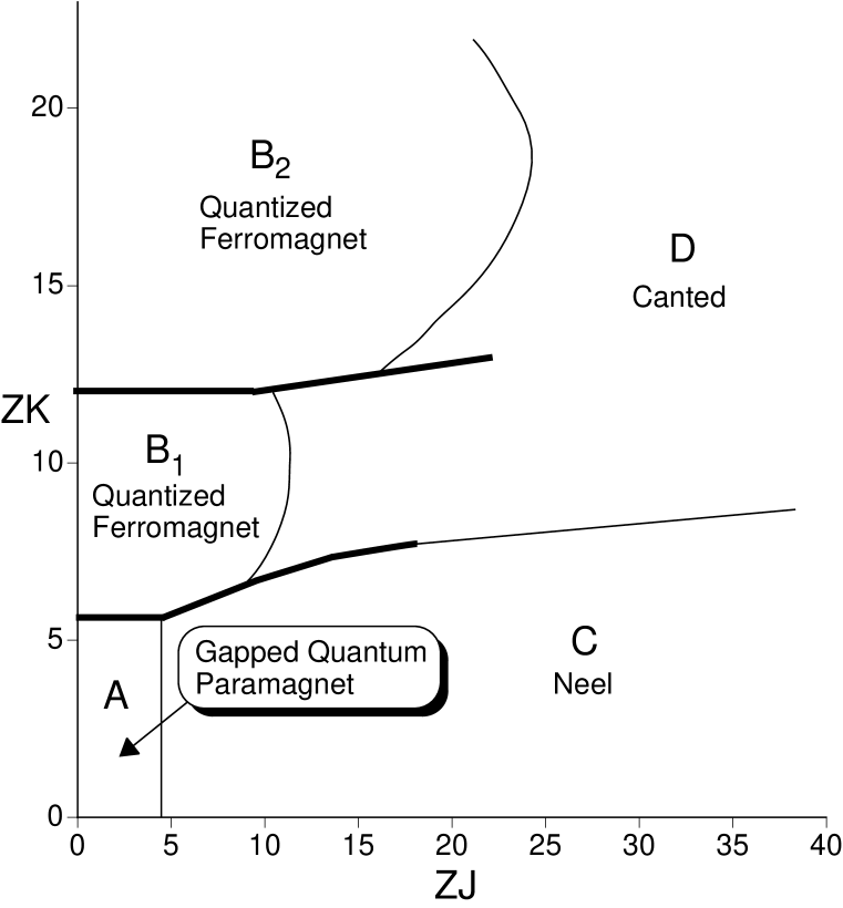
FIG. 1.: Mean-field phase diagram of $\hat{H}$ (Eqn 3) as a function of the couplings $J$ and $K$ at $MZ=4$, $g=1$, and $\alpha=1/2$; $Z$ is the co-ordination number of the lattice. The model does not have ${\cal P}$ symmetry at these values, but the phase diagram for the ${\cal P}$ symmetric case is very similar. The mean-field result becomes exact in the limit of large spatial dimensionality, but the general features of the phase diagram are expected to hold for all $d>1$. Thin lines represent second-order transitions while thick lines are first order. The quantized ferromagnetic phases $\rm{B}_{\ell}$ have magnetic moment per site $\ell$; there is an infinite sequence of these phases for all integers $\ell>0$ at larger values of $K$, and only the first two are shown. The phases have the following ground state expectation values, up to a global $O(3)$ rotation: (A) $\langle\hat{L}_{\mu}\rangle=0$, $\langle\hat{n}_{\mu}\rangle=0$; ($\rm{B}_{\ell}$) $\langle\hat{L}_{z}\rangle=\ell$, $\langle\hat{n}_{z}\rangle\neq 0$, $\langle\hat{L}_{x,y}\rangle=0$, $\langle\hat{n}_{x,y}\rangle=0$; (C) $\langle\hat{L}_{\mu}\rangle=0$, $\langle\hat{n}_{z}\rangle\neq 0$, $\langle\hat{n}_{x,y}\rangle=0$; (D) $\langle\hat{L}_{x,z}\rangle\neq 0$, $\langle\hat{n}_{x,z}\rangle\neq 0$, $\langle\hat{L}_{y}\rangle=0$, $\langle\hat{n}_{y}\rangle=0$.

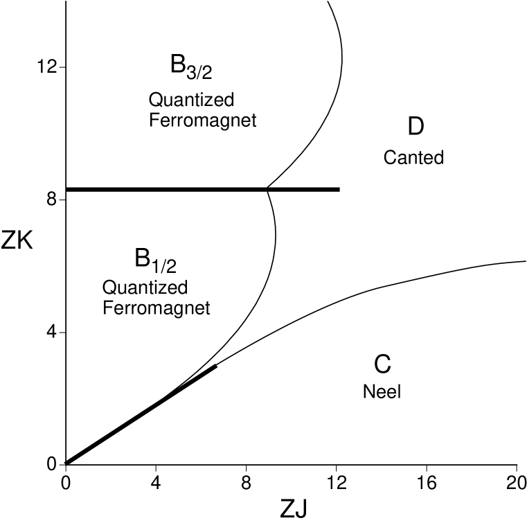
FIG. 2.: Mean-field phase diagram of $\hat{H}$ with $\hat{L}_{\mu}$ given by (109), monopole charge $q=1/2$, $M=0$ and other parameters and conventions are as in Fig 1. The phases have the same physical properties as those of the corresponding phases in Fig 1. The moment, $\ell$, of the quantized ferromagnet phases $\rm{B}_{\ell}$ is now half-integral, and such phases exist for all half-integers $\ell$ at larger $K$. The model is on a bi- partite lattice, and the expectation values (up to a global $O(3)$ rotation) in the various phases on the two sublattices, 1,2, are: ($\rm{B}_{\ell}$) $\langle\hat{L}_{1z}\rangle=\langle\hat{L}_{2z}\rangle=\ell$, $\langle\hat{n}_{1z}\rangle=-\langle\hat{n}_{2z}\rangle\neq 0$, $\langle\hat{L}_{1x,1y,2x,2y}\rangle=0$, $\langle\hat{n}_{1x,1y,2x,2y}\rangle=0$; (C) $\langle\hat{L}_{1x}\rangle=-\langle\hat{L}_{2x}\rangle\neq 0$, $\langle\hat{n}_{1x}\rangle=\langle\hat{n}_{2x}\rangle\neq 0$, $\langle\hat{L}_{1y,1z,2y,2z}\rangle=0$, $\langle\hat{n}_{1y,1z,2y,2z}\rangle=0$; (D) $\langle\hat{L}_{1z}\rangle=\langle\hat{L}_{2z}\rangle\neq 0$, $\langle\hat{n}_{1z}\rangle=-\langle\hat{n}_{2z}\rangle\neq 0$, $\langle\hat{L}_{1x}\rangle=-\langle\hat{L}_{2x}\rangle\neq 0$, $\langle\hat{n}_{1x}\rangle=\langle\hat{n}_{2x}\rangle\neq 0$, $\langle\hat{L}_{1y,2y}\rangle=0$, $\langle\hat{n}_{1y,2y}\rangle=0$;

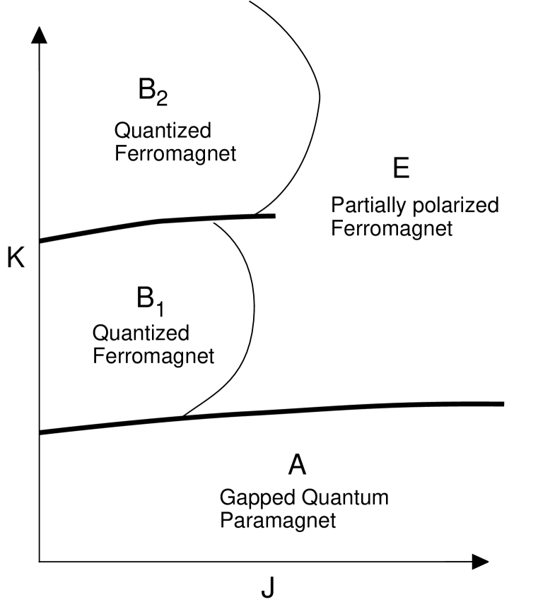
FIG. 3.: Expected phase diagram of $\cal{H}$ in $d=1$ with monopole charge $q=0$. The phases A and $\rm{B}_{\ell}$ are as in Fig 1. The $d>1$ phase D becomes phase E in $d=1$; the latter phase has $\langle\hat{n}_{\mu}\rangle=0$, $\langle\hat{L}_{z}\rangle\neq 0$, $\langle\hat{L}_{x,y}\rangle=0$. The magnetic moment is not quantized but varies continuously. The $\hat{n}_{x,y}$ fields have algebraic correlations in space.

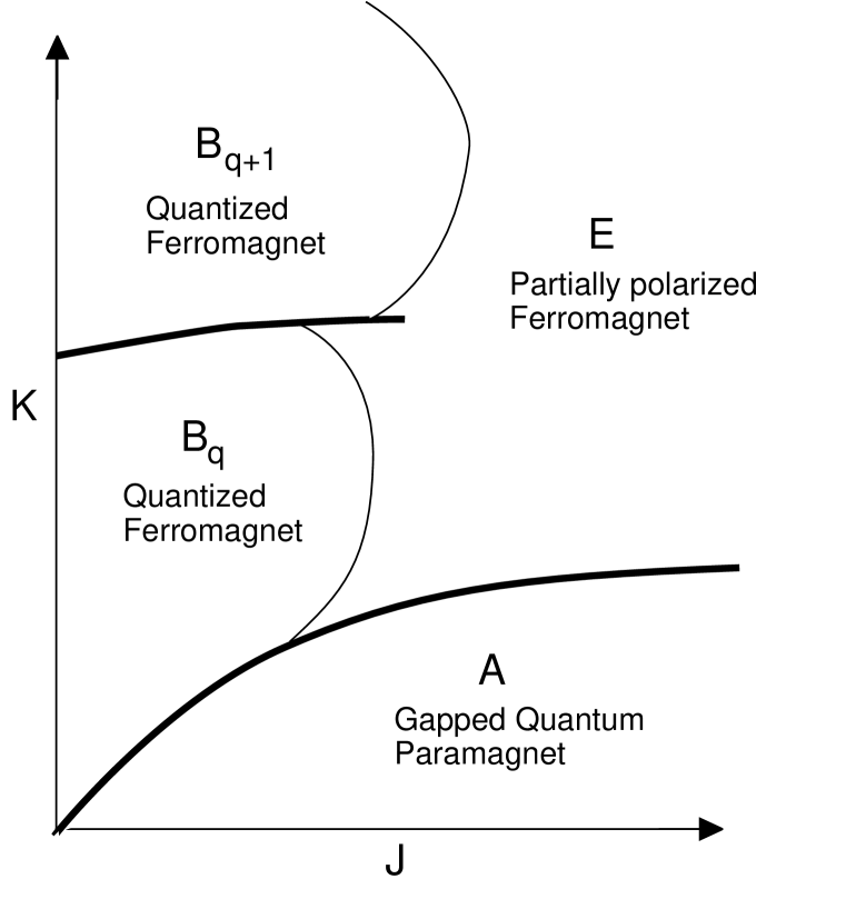
FIG. 4.: Expected phase diagram of $\cal{H}$ in $d=1$ with monopole charge an integer $q>0$. Phases are similar to those with the same labels in Fig 2 and 3.

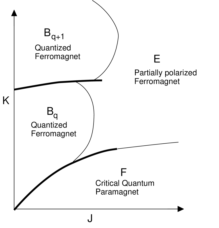
FIG. 5.: Expected phase diagram of $\cal{H}$ in $d=1$ with monopole charge a half-integer $q>0$. Phases are similar to those with the same labels in Fig 2 and 3. Phase F has no broken symmetry and algebraic correlations of all spin operators. Its low energy properties are described by the $1+1$ dimensional $O(3)$ non-linear sigma model with a topological term with co-efficient $\theta=\pi$.

REFERENCES

- [1] E.C. Stoner, Proc. Roy. Soc. (London) A 154, 656 (1936).
- [2] S. Sachdev, Z. Phys. B 94, 469 (1994).
- [3] C. Pfleiderer, G.J. McMullan, and G.G. Lonzarich, Physica B 206 & 207, 847 (1995).
- [4] J.A. Hertz, Phys. Rev. B 14, 525 (1976).
- [5] A.J. Millis, Phys. Rev. B 48, 7183 (1993).
- [6] S. Sachdev, A.V. Chubukov and A. Sokol, Phys. Rev. B, 51, 14874 (1995).
- [7] P.C. Hohenberg and J.B. Swift, J. Phys. C 7, 4009 (1974).
- [8] P. Fulde and I. Peschel, Adv. Phys. 21, 1 (1972); R.J. Birgeneau, J. Als-Nielsen and E. Bucher, Phys. Rev. Lett. 27, 1530 (1971).
- [9] S. Jin, T.H. Tiefel, M. McCormack, R.A. Fastnacht, R. Ramesh, and L.H. Chen, Science, 264, 413 (1994).
- [10] N. Furukawa, J. Phys. Soc. Jpn. 63, 3214 (1994); preprints cond-mat/9505011 and cond-mat/9505034; A.J. Millis, P.B. Littlewood, and B.I. Shraiman, Phys. Rev. Lett. 74, 5144 (1995).
- [11] S.E. Barrett et al., Phys. Rev. Lett. 72, 1368 (1994); ibid 74, 5112 (1995); R. Tycko et al., Science 268, 1460 (1995).
- [12] D.-H. Lee and C.L. Kane, Phys. Rev. Lett. 64, 1313 (1990).
- [13] H.A. Fertig, L. Brey, R. Cote, and A.H. MacDonald, Phys. Rev. B50, 11018 (1994).
- [14] S.L. Sondhi, A. Karlhede, S.A. Kivelson and E.H. Rezayi, Phys. Rev. B 47, 16419 (1993).
- [15] M. Kasner and A.H. MacDonald, cond-mat/9510021
- [16] N. Read and S. Sachdev, Phys. Rev. Lett. 75, 3509 (1995).
- [17] L. Brey, H.A. Fertig, R. Cote, and A.H. MacDonald, Phys. Rev. Lett. 75, 2562 (1995).
- [18] N. Read, private communication.
- [19] T.R. Kirkpatrick and D. Belitz, cond-mat/9601008.
- [20] C.J. Hamer, J.B. Kogut, and L. Susskind, Phys. Rev. D 19, 3091 (1979).
- [21] S. Chakravarty, B.I. Halperin, and D.R. Nelson, Phys. Rev. Lett.60, 1057 (1988); Phys. Rev. B39, 2344 (1989).
- [22] S. Sachdev and J. Ye, Phys. Rev. Lett. 69, 2411 (1992); A.V. Chubukov and S. Sachdev, Phys. Rev. Lett. 71, 169 (1993); A.V. Chubukov, S. Sachdev, and J. Ye, Phys. Rev. B 49, 11919 (1994).
- [23] J. Ye, S. Sachdev, and N. Read, Phys. Rev. Lett. 70, 4011 (1993); N. Read, S. Sachdev and J. Ye, Phys. Rev. B, 52, 384 (1995).
- [24] A. J. Millis and H. Monien, Phys. Rev. Lett. 70, 2810 (1993); Phys. Rev. B 50, 16606 (1994); J. M. Tranquada, G. Shirane, B. Keimer, S. Shamoto, and M. Sato, Phys. Rev. B 40, 4503 (1989).; A.W. Sandvik and D.J. Scalapino, Phys. Rev. Lett. 72, 2777 (1994); A.W. Sandvik, A.V. Chubukov and S. Sachdev, Phys. Rev. B, 51, 16483 (1995).
- [25] M.P.A. Fisher, P.B. Weichmann, G. Grinstein, and D.S. Fisher, Phys. Rev. B 40, 546 (1989).
- [26] We could also have studied an analogous “quantum top model” to allow for the possibility of phases in which the spins are non-collinear but have no net ferromagnetic moment—the analog of the Néel phase in that model would have 3 spin-wave modes, all with . The phases with a ferromagnetic moment in the quantum top model are quite similar to those being discussed here in the quantum rotor model, and we will therefore not enter into this complication in this paper.
- [27] E. Brezin and J. Zinn-Justin, Phys. Rev. B 14, 3110 (1976). D.R. Nelson and R.A. Pelcovits, Phys. Rev. B 16, 2191 (1977).
- [28] See e.g. D. Boyanovsky and J.L. Cardy, Phys. Rev. B 26, 154 (1982).
- [29] S. Sachdev, T. Senthil, and R. Shankar, Phys. Rev. B 50, 258 (1994).
- [30] The limits of momentum and frequency going to zero do not commute in the computation of the effective coupling of to ; it is necessary to generalize to a momentum- and frequency-dependent field and take the limit before taking .
- [31] R. Shankar and N. Read, Nucl. Phys. B336, 457 (1990).
- [32] T.T. Wu and C.N. Yang, Nucl. Phys. B107, 365 (1976).
- [33] I. Affleck and F.D.M. Haldane, Phys. Rev. B 36, 5291 (1987).
- [34] E. Witten, Comm. Math. Phys. 92, 455 (1984); V.G. Knizhnik and A.B. Zamalodchikov, Nucl. Phys. B 247, 83 (1984).
- [35] Because systems with do not have symmetry, terms which couple the ‘spin’ field (in the notation of Ref [33]) with the magnetization density are also permitted. It may be necessary to include this term in the most general case.
- [36] I. Affleck, in Les Houches XLIX, Fields, Strings and Critical Phenomena, edited by E. Brezin and J. Zinn Justin, pg 562, North Holland, Amsterdam (1990).
- [37] S. Sachdev in Proceedings of the 19th IUPAP International Conference on Statistical Physics, edited by B.-L. Hao, World Scientific, Singapore, to be published; cond-mat/9508080
- [38] M. Aizenman and J. Wehr, Phys. Rev. Lett. 62, 2503 (1989); K. Hui and A.N. Berker, ibid 62, 2507 (1989).
- [39] E. Brezin, J.C. Le Guillou and J. Zinn-Justin in Phase Transitions and Critical Phenomena vol 6, edited by C. Domb and M.S. Green, Academic Press, London (1976).