Zero–Bias Anomaly in Finite Size Systems

Abstract

The small energy anomaly in the single particle density of states of disordered interacting systems is studied for the zero dimensional case. This anomaly interpolates between the non–perturbative Coulomb blockade and the perturbative limit, the latter being an extension of the Altshuler–Aronov zero bias anomaly at $d=0$. Coupling of the zero dimensional system to a dissipative environment leads to effective screening of the interaction and a modification of the density of states.

I Introduction

The density of states (DOS) of disordered interacting electronic systems exhibits singularity near the Fermi energy. This phenomenon manifests itself in the suppression of the tunneling conductance at small external bias and is referred to as zero bias anomaly (ZBA). It has been explained and investigated theoretically by Altshuler and Aronov (AA) in 1979 for $d=3$ and latter extended for lower dimensionality by Altshuler Aronov and Lee [1](for a review see Ref. [2]). They have predicted that for a d–dimensional system with diffusive disorder and weak short range interactions the singular correction to the DOS behaves as $\delta\nu_{d}\sim(\mbox{max}\{\epsilon,T\})^{d/2-1}$ with the dimensionality $d=1,2,3$. For three dimensional ($d=3$) samples the ZBA constitutes a small but nonanalytic correction to the DOS (as long as the dimensionless conductance, $g$, is large, $g\gg 1$). It may be argued subsequently that this phenomenon is a precursor of the “Coulomb gap”, which appears in the Anderson insulator regime, $g<1$. Throughout this paper we shall consider good conductors, hence we shall not discuss here the localized regime. But remarkably enough, even for good metals, $g\gg 1$, there is a situation where the ZBA is a strong effect. This is the case with a finite size system. The original treatment of AA was given for infinite (quasi) d–dimensional systems. For a finite size system the quantization of the spectrum of the diffusive modes becomes of crucial importance. For instance, the electron–electron interaction term in the Hamiltonian takes the form

$$H_{int}=\frac{1}{2}\sum_{\bf Q}V({\bf Q}):\rho_{\bf Q}\rho_{-{\bf Q}}:,$$ (1)

where ${\bf Q}=2\pi{\bf n}/L$ are quantized momenta, $\rho_{\bf Q}$ is the ${\bf Q}$ component of the electron density operator and $:\ldots:$ denotes normal ordering. The quantization of the momentum has two major consequences for the ZBA.

First, if one accounts for all finite ${\bf Q}$, excluding the ${\bf Q}=0$ mode, in the interaction Hamiltonian, the singularity in the DOS is rounded off on the scale $\mbox{max}\{\epsilon,T\}\approx E_{c}$, where $E_{c}$ is the Thouless correlation energy. As long as the ZBA is still a small correction to the total DOS on the scale $E_{c}$, $\delta\nu_{d}(E_{c})\ll\nu^{[0]}$, the finite ${\bf Q}$ modes do not enhance the singularity for $\epsilon,T<E_{c}$. It is easy to see [2] that the requirement $\delta\nu_{d}(E_{c})\ll\nu^{[0]}$ is satisfied for $g\gg 1$; in this case the finite ${\bf Q}$ contribution to the ZBA is small for any energy and temperature. It means that for such systems the finite ${\bf Q}$ interaction may indeed be treated by perturbation theory, which produces regular expansion in powers of $1/g$. Throughout this paper we shall assume that the condition $g\gg 1$ is satisfied, hence the perturbative treatment of the non–zero modes is applicable.

The second consequence of the spectrum quantization is the special role played by the ${\bf Q}=0$ term in the interaction Hamiltonian. Its contribution to the energy may be written as $V(0):N^{2}:/2$, where $N\equiv\rho_{0}$ is the total number of electrons in a dot. This term in fact corresponds to the classical charging energy of the dot. It leads to a strong singularity in the DOS. The first order in interaction perturbative result is $\delta\nu_{0}(\epsilon=0)=-V(0)/(4T)$ (for the ${\bf Q}=0$ contribution $T$ and $\epsilon$ are not interchangeable). In the limit $T<V(0)$, the perturbative treatment is not sufficient. We present here a relatively simple method which allows us to treat ${\bf Q}=0$ contribution to the ZBA exactly. An exact solution is possible due to the fact that the zero–mode interaction term commutes with the total Hamiltonian. As a result the problem is trivial, although the zero–mode interaction has some interesting consequences. The thermodynamical and the response functions are practically unaffected by the zero–mode interactions (apart from modifying the statistical ensemble from grand canonical to canonical). The single particle DOS is modified in an essential way. We use imaginary time functional integral to integrate out all fermionic degrees of freedom. Similar methods were used in the context of Josephson junctions with dissipative environment (for a review see [3]). Non–perturbative treatment reveals the exponential suppression of the DOS at the Fermi energy. This result reproduces the classical treatment of the “orthodox” theory of the Coulomb blockade [4]. In other words, the $d=0$ generalization of the AA ZBA, and the Coulomb blockade, are two limiting cases of the same theory.

This statement is in fact not new. In his original paper, Ref. [5], Nazarov had established the connection between the two (including a non–perturbative treatment of the finite ${\bf Q}$ modes). A similar, although more transparent, theory has recently been put forward by Levitov and Shytov [6]. To a large extent, our results can be extracted as the $d=0$ limit of the expressions found in Refs. [5, 6]. The point is that Refs. [5, 6] used some uncontrolled (although plausible) approximations. We have shown that for ${\bf Q}=0$ all calculations may be done exactly, confirming some of the approximations made in Refs. [5, 6].

One may combine the zero and finite ${\bf Q}$ mode interactions to the ZBA. In doing so we take into account the zero mode in an exact fashion and add on top of it the perturbative contribution of the ${\bf Q}\neq 0$ modes. As was mentioned above the latter can be expressed as a regular expansion in powers of $1/g$ valid at any temperature energy and dimensionality. To address the insulating regime one should consult Refs. [5, 6]. In the metallic limit the ${\bf Q}\neq 0$ contribution modifies the DOS at high energies ($\epsilon\geq e^{2}/2C$), as a precursor to the Coulomb blockade which dominates at lower energies (cf. Fig. 4b).

The new ingredient in our analysis is the inclusion of the zero–point (and thermal) motion of the electromagnetic environment in contact with the system. We show that the influence of the environment may lead to a Debye screening of the zero–mode interaction, hence to a softening of the Coulomb blockade. The physics behind the zero–mode screening is the following: the total charge on the dot, $eN$, interacts with charges in the environment, leading to their redistribution. The polarized charge of the environment reduces the energy cost of adding (or removing) an electron to (or from) the dot. There is a certain finite time constant (the $RC$ – constant of the circuit), characterizing this redistribution of the environmental charge, rendering the effective interaction in the dot non–instantaneous (retarded). It might appear that the results obtained through this analysis are highly non–universal and depend on the particular choice of the model for the environment. We stress, however, that our result expressed by Eqs. (23) and (36) is quite general, the only model–dependent feature is the concrete form of the screened zero–mode interaction, $V(\omega)$. Nonuniversality in this sense is unavoidable, due to the long range nature of the Coulomb interaction: the behavior of the dot depends on numerous long distance features.

A particularly interesting case is when the zero–mode interaction is fully screened in the long time limit. By this we refer to a situation when on a long time scale the addition of an electron to the dot does not cost any energy (for instance there is a slow continuous leakage of any extra charge from the dot). In this case the usual Coulomb gap in the spectrum is absent and one obtains the power–law ZBA, very similar to the one known from the physics of Luttinger liquid. The exponent is determined by the time scale of the environment polarization. This result for a quantum dot coincide with those obtained in Refs. [7, 8] for a single tunnel junction connected to a linear $RCL$ circuit [9]. For a quantum dot one may consider the setup with only partially screened interaction, where the gap in the DOS at low energies crosses over to a power–law ZBA at larger energies.

Let us list several aspects of the problem, which we do not consider here. Although we deal with finite size systems, we do not consider effects related to the discreteness of the single electron spectrum. It means that the mean level spacing, $\Delta$, is assumed to be the smallest energy scale in our problem. We restrict ourselves to the case of good metals, where $g=E_{c}/\Delta\gg 1$. Thus the energy interval of interest, $\Delta<\epsilon<E_{c}$, is wide. Since we are not interested in the single electron spectrum quantization, one may choose any boundary conditions for the electron wave functions. We prefer to use periodic boundary conditions and employ the momentum representation. We also stress that our analysis omits the underlaying periodicity of the problem as function of the charge of the positive background (or of a gate voltage) which could be manifested as a sequence of Coulomb blockade resonances. Instead we restrict ourselves to the case where the background is such that the dot prefers to have an integer charge (half way between resonances). One can easily generalize the same treatment for any background charge, noting that in the close vicinity of a half–integer (near a resonance) a very different treatment, accounting for multiple tunneling events [10] is required. In fact even far from resonances multiple tunneling may be important (e.g “inelastic co–tunneling” [11]). For the sake of clarity we restrict ourselves to a “golden rule” scenario, where we consider only lowest order processes in the tunneling amplitude, postponing the consideration of multiple tunneling to a further publication.

The outline of the article is as follows. In Section II we recall the derivation of the ZBA given by AA and extend it to $d=0$. The non–perturbative treatment of zero-mode interaction is discussed in Section III, where we study in some details the case of an instantaneous zero–mode interaction and rederive the results of the “orthodox” Coulomb blockade. Section IV is devoted to the study of screened retarded zero–mode interaction. We show that in one particular case the ZBA reproduces the results derived for a single junction connected to a linear circuit.

II Zero–Bias Anomaly

The derivation of the ZBA in the diffusive interacting systems proceeds as follows [2]. One calculates the single particle (not to be confused with the thermodynamic, $dn/d\mu$) density of states as function of energy or temperature. The single particle DOS is defined as the imaginary part of the trace of the single particle Green function

$$\nu(\epsilon)=-\left.\frac{1}{\pi}\Im\mbox{Tr}{\cal G}(\epsilon_{n})\right|_{i\epsilon_{n}\rightarrow\epsilon+i\delta}.$$ (2)

Following AA [2], we calculate the first order correction in the screened interaction to the single particle DOS in a dirty system. The dominant contribution [12] comes from the exchange diagram depicted in Fig. 1.

FIG. 1.: First order interaction correction to the Green function; wavy line – interaction; dashed lines – impurity dressing (diffusons).

After performing the fast momentum summation one obtains

$$\delta\nu(\epsilon)=-\frac{\nu^{[0]}}{\pi}\Im\,T\!\!\!\!\!\sum_{\omega_{m}>\epsilon_{n}}\sum_{\bf Q}\left.\frac{2\pi iV({\bf Q},\omega_{m})}{(D{\bf Q}^{2}+|\omega_{m}|+\gamma_{in})^{2}}\right|_{i\epsilon_{n}\rightarrow\epsilon+i\delta},$$ (3)

where $D$ is the diffusion constant; $\gamma_{in}$ – the inelastic relaxation rate; $V({\bf Q},\omega_{m})$ – the screened Coulomb interaction, given by

$$\left[V({\bf Q},\omega_{m})\right]^{-1}=\left[V^{[0]}({\bf Q})\right]^{-1}+\Pi({\bf Q},\omega_{m})$$ (4)

Here $V^{[0]}({\bf Q})$ is the bare (instantaneous) Coulomb interaction and $\Pi({\bf Q},\omega_{m})$ is the polarization operator of the system. For an isolated diffusive system the polarization is

$$\Pi({\bf Q},\omega_{m})=\nu^{[0]}\frac{D{\bf Q}^{2}}{D{\bf Q}^{2}+|\omega_{m}|};$$ (5)

$\nu^{[0]}$ is the DOS of non–interacting system.

Let us consider a three dimensional cube with the linear size $L$ with no current flowing through the boundaries. The slow momentum ${\bf Q}$ assumes quantized values

$${\bf Q}=\frac{2\pi}{L}{\bf n},$$

where ${\bf n}$ is a vector with integer components, including ${\bf n}=(0,0,0)$. If either the energy, $\epsilon$, or the temperature, $T$, is much larger than the Thouless energy, $E_{c}\equiv D/L^{2}$, one may disregard the discreteness of ${\bf Q}$ and perform slow momentum integration instead of summation. We shall refer to such a case as a three–dimensional, $d=3$. Substituting Eqs. (4) and (5) in Eq. (3) and performing integrations, one readily obtains [2] (e.g. for $T\gg E_{c};\epsilon$)

$$\frac{\delta\nu_{3}}{\nu^{[0]}}=a_{3}\frac{1}{g}\sqrt{\frac{T}{E_{c}}},$$ (6)

where $a_{3}\approx 3.8\cdot 10^{-2}$ and $g\equiv\nu^{[0]}DL^{d-2}\gg 1$ is the dimensionless conductance of the sample (the full $T$ and $\epsilon$ dependence may be found in Ref. [2]). At small temperature this correction exhibits singular (non–analytic) behavior, which is the ZBA. One cannot employ, however, Eq. (6) for $\epsilon;T<E_{c}$. In this case the discreteness of the momentum spectrum begins to play a crucial role. Performing momentum summation in Eq. (3), excluding the ${\bf Q}=0$ contribution, one obtains for $\gamma_{in}\ll\epsilon;T\ll E_{c}$

$$\frac{\delta\nu_{3}}{\nu^{[0]}}=a_{0}\frac{1}{g}\left(\frac{T}{E_{c}}\right)^{2}f_{0}\left(\frac{\epsilon}{T}\right),$$ (7)

where $a_{0}=\sum_{{\bf n}\neq 0}(2\pi|{\bf n}|)^{-6}\approx 1.1\cdot 10^{-3}$ and

$$f_{0}(x)=\int_{0}^{\infty}\!\!dyy\left(2-\mbox{tanh}\frac{y-x}{2}-\mbox{tanh}\frac{y+x}{2}\right)$$

with the asymptotic values $f_{0}(x\ll 1)=\pi^{2}/3\,$; $f_{0}(x\gg 1)=x^{2}$. At $T\approx E_{c}$ Eqs. (6) and (7) match parametrically. According to Eq. (7) the small temperature singularity in the DOS is rounded off due to finite size effects (the finite value of $E_{c}$), (Fig. 2).

Eq. (7) does not account, however, for the ${\bf Q}=0$ contribution to the momentum sum in Eq. (3). Below we evaluate this contribution and argue that it reflects the physics of the Coulomb blockade. The first problem is that the bare Coulomb interaction, $V^{[0]}({\bf Q})=L^{-3}4\pi e^{2}/Q^{2}$, is not well–defined for ${\bf Q}=0$. We argue that for finite size samples this expression should be regularized at $Q\approx 1/L$ (cf. analogous regularization of the bare interaction in the $d=1$ case [2]), leading to $V^{[0]}({\bf Q}=0)\approx e^{2}/L$. More precisely we shall use

$$V^{[0]}=\frac{e^{2}}{C},$$ (8)

where $C\approx L$ is the self capacitance of the sample, which includes some non–universal geometrical factors (hereafter the interaction potential, $V$, without momentum index refers to ${\bf Q}=0$). In other words, one may regard the finite value of $V^{[0]}$ as the result of fast screening processes, occurring on the boundary of the sample, which are not included explicitly in Eq. (4). According to Eqs. (4) and (5), the ${\bf Q}=0$ interaction can not be screened, indeed $\Pi({\bf Q}=0,\omega_{m})=0$. This amounts to saying that a finite size isolated system cannot screen its total charge. This is not the case for a system which is coupled capacitevely to the environment. In the latter case the polarization operator should contain an additional term arising from the polarization of the environment. This would lead to an effective screening of the ${\bf Q}=0$ interaction. We postpone, however, discussion of the screened zero–mode interaction till Section IV and proceed with the interaction given by Eq. (8).

FIG. 2.: Perturbative calculation of the DOS. Full line: ${\bf Q}\neq 0$ modes only; dashed line: ${\bf Q}=0$ mode is included. Dotted line: AA result without account for finite size effects ($d=3$, cf. Eq. (6)). The curves are shifted vertically for clarity.

Substituting now Eq. (8) into Eq. (3) and performing energy summation and analytical continuation, one obtains for the zero–mode contribution to the DOS

$$\frac{\delta\nu_{0}}{\nu^{[0]}}=-\frac{V^{[0]}}{2\pi^{2}T}\Re\,\Psi^{(\prime)}\left(\frac{1}{2}+\frac{\gamma_{in}-i\epsilon}{2\pi T}\right),$$ (9)

where $\Psi(x)$ is the digamma function. For $\gamma_{in}\ll T$ this reduces to

$$\frac{\delta\nu_{0}}{\nu^{[0]}}=-\frac{V^{[0]}}{4T}\mbox{cosh}^{-2}\frac{\epsilon}{2T}.$$ (10)

Note that the dependencies on temperature and energy are very different, whereas for finite $d$ energy and temperature play essentially the same role. The temperature (and diffusive constant) dependence is compatible with the AA result, $\delta\nu_{d}\sim T^{(d/2-1)}D^{-d/2}$, extended to $d=0$. The zero–mode contribution leads to a dramatic singularity $\sim T^{-1}$ in the single particle DOS, Fig. 2. For sufficiently low temperatures, $T\ll e^{2}/2C$, this last expression cannot be correct. Indeed in this case Eq. (10) predicts $\delta\nu\gg\nu^{[0]}$, a result which is certainly nonperturbative. Moreover, the resulting DOS becomes negative. This clearly indicates that the first order perturbation theory is not sufficient to treat the ZBA in finite size systems at low temperatures. In the next section we shall show how the zero–mode interaction can be treated nonperturbativly. Unlike Eq. (10), the exact result is well behaved at any temperature and, in fact, is well known from the “orthodox” theory of the Coulomb blockade [4].

III Zero mode interaction

A General formulation

As we have seen in the previous section, the perturbative treatment of the zero–mode interactions in a dot at low temperature meets serious difficulties. From another hand, the first order (in the screened interaction) result for ${\bf Q}\neq 0$ and a not too dirty system, $g\gg 1$ (cf. Eq. (6), (7)), is well behaved. Thus we separate out the dangerous contribution of the zero–mode interaction and try to treat it non–perturbativly. To this end consider a Hamiltonian describing electrons moving in a disordered potential, which interact through the zero mode repulsive interaction only

$$H_{0}=\sum_{\alpha}\epsilon_{\alpha}a^{+}_{\alpha}a_{\alpha}+\frac{V^{[0]}}{2}:\left[\sum_{\alpha}a^{+}_{\alpha}a_{\alpha}-N_{0}\right]^{2}:\,,$$ (11)

where $a^{+}_{\alpha}(a_{\alpha})$ is a creation (annihilation) operator of an electron in an exact single particle state (which is defined including disorder potential and spin) with an eigenenergy $\epsilon_{\alpha}$; $V^{[0]}$ is the bare zero–mode interaction, Eq. (8); $N_{0}$ - the charge of the positive background, which we assume to be an integer [13]. Bellow we shall comment on the case where Hamiltonian includes also finite ${\bf Q}$ interactions, which can be treated perturbatively.

Before to proceed we would like to stress the following fact. One may argue that the interaction term in the Hamiltonian, Eq. (11), is trivial. Indeed it has the form $H_{int}=V^{[0]}:N^{2}:/2$, where $N\equiv\sum_{\alpha}a^{+}_{\alpha}a_{\alpha}$ is a total number of particles in the system. As $N$ commutes with the Hamiltonian, $[H_{0},N]=0$, it does not have any dynamics, $\partial_{t}N=0$. Thus the interaction term is just a constant added to the Hamiltonian, and seems not to have any nontrivial consequences. This is indeed the case when considering thermodynamical properties or response functions of the isolated dot. It is, however, not the case with the single particle Green function, which correlates the amplitude of the creation of one additional electron at an initial time, $t_{i}$, and its subsequent destruction at time $t_{f}$. Thus any measurement of the single particle Green function assumes implicitly the existence of processes which do not conserve the number of particles in a dot (e.g. due to tunneling). Such processes render the entire Hamiltonian noncommuting with the particle number. As a result the $N^{2}$ interaction term has a significant impact on the single particle Green function. After completing the calculations we shall comment on the relation of the above arguments to gauge invariance.

The imaginary time single particle Green function may be written as [14]

$${\cal G}_{\alpha}(\tau_{i},\tau_{f},\mu)=\frac{1}{Z(\mu)}\int{\cal D}[\psi^{*}_{\alpha}(\tau)\psi_{\alpha}(\tau)]e^{-S[\psi^{*}_{\alpha},\psi_{\alpha}]}\psi^{*}_{\alpha}(\tau_{i})\psi_{\alpha}(\tau_{f}),$$ (12)

with the fermionic action given by

$$S[\psi^{*}_{\alpha},\psi_{\alpha}]=\int_{0}^{\beta}d\tau\left[\sum_{\alpha}\psi^{*}_{\alpha}(\tau)(\partial_{\tau}+\epsilon_{\alpha}-\mu)\psi_{\alpha}(\tau)+\frac{V^{[0]}}{2}\left[\sum_{\alpha}\psi^{*}_{\alpha}(\tau)\psi_{\alpha}(\tau)-N_{0}\right]^{2}\right];$$ (13)

here $Z(\mu)$ is the partition function and $\mu$ is the chemical potential. Splitting the interaction term in the action by means of the Hubbard–Stratonovich transformation with the auxiliary Bose field, $\phi(\tau)$, one obtains

$${\cal G}_{\alpha}(\tau_{i}-\tau_{f})=\frac{1}{Z(\mu)} \int{\cal D}[\phi(\tau)]e^{-\int_{0}^{\beta}d\tau\left[\phi(\tau)[2V^{[0]}]^{-1}\phi(\tau)-iN_{0}\phi(\tau)\right]}$$ (15)

$$\int{\cal D}[\psi^{*}_{\alpha}\psi_{\alpha}]e^{-\int_{0}^{\beta}d\tau\sum_{\alpha}\psi^{*}_{\alpha}(\partial_{\tau}+\epsilon_{\alpha}-\mu+i\phi(\tau))\psi_{\alpha}}\psi^{*}_{\alpha}(\tau_{i})\psi_{\alpha}(\tau_{f})$$

$$=\frac{1}{Z(\mu)} \int{\cal D}[\phi(\tau)]e^{-\int_{0}^{\beta}d\tau\left[\phi(\tau)[2V^{[0]}]^{-1}\phi(\tau)-iN_{0}\phi(\tau)\right]}Z^{[\phi]}(\mu){\cal G}^{[\phi]}_{\alpha}(\tau_{i},\tau_{f},\mu)$$ (16)

with the same transformations in $Z(\mu)$. Here $Z^{[\phi]}(\mu)$ and ${\cal G}^{[\phi]}_{\alpha}(\tau_{i},\tau_{f},\mu)$ are respectively the partition and Green functions of non–interacting electrons in the time dependent (but spatially uniform) potential, $i\phi(\tau)$. To calculate these quantities one should resolve the spectral problem for the first order differential operator $\left[\partial_{\tau}-\mu+\epsilon_{\alpha}+i\phi(\tau)\right]$ with antiperiodic boundary conditions. This can be easily done (see e.g. chapter 7 in Ref. [14]). For the spectral determinant (partition function) one finds

$$Z^{[\phi]}(\mu)=Z^{[0]}(\mu-i\phi_{0}),$$ (17)

where $Z^{[0]}(\mu)\equiv\exp\{-\beta\Omega^{[0]}(\mu)\}$ is the partition function of non–interacting electron gas. We have introduced Matsubara representation for the boson field, $\phi(\tau)$: $\phi_{m}\equiv\beta^{-1}\int_{0}^{\beta}d\tau\phi(\tau)\exp\{i\omega_{m}\tau\}$, $\omega_{m}=2\pi mT$. The Green function is given by

$${\cal G}^{[\phi]}_{\alpha}(\tau_{i},\tau_{f},\mu)={\cal G}^{[0]}_{\alpha}(\tau_{i}-\tau_{f},\mu-i\phi_{0})e^{i\int_{\tau_{i}}^{\tau_{f}}d\tau[\phi(\tau)-\phi_{0}]},$$ (18)

where ${\cal G}^{[0]}_{\alpha}(\epsilon_{n},\mu)=(i\epsilon_{n}-\epsilon_{\alpha}+\mu)^{-1}$ is the Green function of non-interacting fermions. It is convenient to rewrite the exponent in the last equation in the following form

$$\exp\{i\int_{\tau_{i}}^{\tau_{f}}d\tau[\phi(\tau)-\phi_{0}]\}=\exp\{\beta\sum_{m\neq 0}\frac{\phi_{m}J_{-m}^{\tau_{i},\tau_{f}}}{\omega_{m}}\},$$ (19)

where $J_{m}^{\tau_{i},\tau_{f}}$ is the Matsubara transform of the following function

$$J_{\tau}^{\tau_{i},\tau_{f}}=\delta(\tau-\tau_{i})-\delta(\tau-\tau_{f}).$$ (20)

Transforming next the functional integral over $\phi(\tau)$ to integrals over the Matsubara components, $\phi_{m}$, we obtain

$${\cal G}_{\alpha}(\tau_{i}-\tau_{f})=\frac{1}{Z(\mu)} \int d\phi_{0}e^{-\beta[\phi_{0}[2V^{[0]}]^{-1}\phi_{0}-i\phi_{0}N_{0}+\Omega^{[0]}(\mu-i\phi_{0})]}{\cal G}^{[0]}_{\alpha}(\tau_{i}-\tau_{f},\mu-i\phi_{0})$$ (22)

$$\int\prod_{m\neq 0}d\phi_{m}\exp\left\{\beta\sum_{m\neq 0}\left[-\frac{\phi_{m}\phi_{-m}}{2V^{[0]}}+\frac{\phi_{m}J_{-m}^{\tau_{i},\tau_{f}}}{\omega_{m}}\right]\right\}.$$

Again with the analogous modifications in $Z(\mu)$. The integral over the static component, $\phi_{0}$, describes the smooth transition between the grand canonical ensemble with the chemical potential $\mu$ (at $V^{[0]}=0$) to the canonical ensemble with $N_{0}$ electrons (at $V^{[0]}=\infty$). For large enough systems ($\Delta^{-1}\equiv-\partial^{2}\Omega^{[0]}/\partial\mu^{2}\gg\beta$) one can neglect differences between the two statistical ensembles. This means that the integral over $\phi_{0}$ can be calculated in a saddle point approximation, leading to ${\cal G}^{[0]}_{\alpha}(\tau_{i}-\tau_{f},\overline{\mu})$, where the stationary point, $\overline{\mu}$, is the real solution of the equation $(\mu-\overline{\mu})/V^{[0]}+N_{0}+\partial\Omega^{[0]}(\overline{\mu})/\partial\mu=0$. The remaining integrals (over $\phi_{m}$ for $m\neq 0$) are purely Gaussian. As a result one obtains

$${\cal G}_{\alpha}(\tau_{i}-\tau_{f},\mu)={\cal G}^{[0]}_{\alpha}(\tau_{i}-\tau_{f},\overline{\mu})e^{-S(\tau_{i}-\tau_{f})},$$ (23)

where

$$S(\tau)=T\sum_{m\neq 0}\frac{V^{[0]}}{\omega_{m}^{2}}(1-e^{i\omega_{m}\tau}).$$ (24)

Eqs. (23) and (24) solve the problem of finding the exact single particle Green function in the presence of the zero–mode interaction. This result is depicted diagrammatically in Fig. 3. The dressed Green function of the interacting problem is given by the bare one (with a renormalized chemical potential) decorated with the propagator of the auxiliary boson field ${\cal D}(\tau)\equiv\exp\{-S(\tau)\}$. We refer to this auxiliary field as a – Coulomb boson. As ${\cal D}(0)=1$, the zero mode interaction does not influence equal time Green functions (apart from the renormalization of the chemical potential). As a result thermodynamical quantities are not affected by the presence of the Coulomb boson. This is not unexpected since the interaction term commutes with a total Hamiltonian, hence it does not affect quantities defined for the closed system. By contrast, to measure a two point Green function one should perform a tunneling experiment, where the system can not be considered as completely isolated. In this case the presence of the interaction term in Eq. (11) (and hence of the Coulomb boson) is of crucial importance.

FIG. 3.: Diagrammatic representation of the Coulomb boson.

This observation can be related to gauge invariance [15]. As we have seen the problem with zero mode interaction is essentially reducible to that of an electrons gas in a spatially uniform a.c. potential. Such a potential can be always removed from the problem by a time–dependent gauge transformation. Thus gauge invariant physical quantities (e.g. thermodynamical quantities) are not affected by the presence of spatially uniform potential, cf. Eq. (17). The single particle Green function, being non gauge invariant object is affected. By introducing an electron tunneling from an external source we fix the (time dependent) phase of the electron wave function in the system. This point has been discussed by Finkelstein [15], who argued that unlike the conductivity or thermodynamical quantities, the non gauge invariant single particle DOS may be affected by very small ${\bf Q}$ terms, leading in $d\leq 2$ to more pronounced singularities.

B The Coulomb boson and DOS

For the instantaneous (frequency–independent) interaction, Eq. (8), the sum in Eq. (24) may be easily performed, yielding

$$S(\tau)=\frac{V^{[0]}}{2}\left(|\tau|-\frac{\tau^{2}}{\beta}\right).$$ (25)

Using the Lehmann representation for temperature Green functions [16] one may write for the propagator of the Coulomb boson

$${\cal D}(\omega_{m})=\int_{-\infty}^{\infty}\frac{d\omega^{\prime}}{2\pi}\frac{B(\omega^{\prime})}{i\omega_{m}-\omega^{\prime}},$$ (26)

where the spectral function $B(\omega)$ is defined as $B(\omega)\equiv-2\Im{\cal D}^{R}(\omega)$. Fourier transforming of ${\cal D}(\tau)=\exp\{-S(\tau)\}$ and analytically continuing we obtain (see Appendix A)

$$B(\omega)=\sqrt{\frac{2\pi}{V^{[0]}T}}\left(e^{-\frac{(\omega+V^{[0]}/2)^{2}}{2V^{[0]}T}}-e^{-\frac{(\omega-V^{[0]}/2)^{2}}{2V^{[0]}T}}\right).$$ (27)

According to Eq. (23) (cf. also Fig. 3) the electron Green function is given by ${\cal G}_{\alpha}(\epsilon_{n})=T\sum_{\omega_{m}}{\cal G}^{[0]}_{\alpha}(\epsilon_{n}-\omega_{m}){\cal D}(\omega_{m})$. Performing the summation by a standard contour integration and then analytical continuation ($i\epsilon_{n}\rightarrow\epsilon+i\delta$) one obtains for the one particle (tunneling) density of states, $\nu(\epsilon)\equiv-\pi^{-1}\sum_{\alpha}\Im{\cal G}^{R}_{\alpha}(\epsilon)$,

$$\nu(\epsilon)=-\frac{1}{2}\int_{-\infty}^{\infty}\frac{d\omega}{2\pi}\left(\mbox{tanh}\frac{\epsilon-\omega}{2T}+\mbox{coth}\frac{\omega}{2T}\right)B(\omega)\nu^{[0]}(\epsilon-\omega),$$ (28)

where $\nu^{[0]}(\epsilon)$ is the density of states in the absence of the zero–mode interaction and $B(\omega)$ is given by Eq. (27). For non–interacting electrons (with or without disorder) $\nu^{[0]}(\epsilon)$ may be well–approximated by a constant value, $\nu^{[0]}$, in this case the integral in the last expression may be readily evaluated. In the limit of weak interaction ($V^{[0]}\ll T$) one obtains

$$\frac{\nu_{0}}{\nu^{[0]}}=1-\frac{V^{[0]}}{4T}\mbox{cosh}^{-2}\frac{\epsilon}{2T}.$$ (29)

This is the zero bias anomaly of AA extrapolated to $d=0$ system, which has been obtained from a diagrammatic expansion, Eq. (10). Notice that we did not actually use the fact that the system is disordered. Note also, that the exact lowest order result, Eq. (29), coincides with the one obtained from the exchange diagram only, Eq. (10). The first order Hartree term with the ${\bf Q}=0$ interaction leads to redefinition of the chemical potential which has been absorbed in the factor, $\overline{\mu}$. For strong interaction ($V^{[0]}\gg T$) one has (Fig. 4a)

$$\frac{\nu_{0}}{\nu^{[0]}}=\left\{\begin{array}[]{ll}{\displaystyle\sqrt{\frac{2\pi T}{V^{[0]}}}\,e^{-\frac{V^{[0]}}{8T}}\mbox{cosh}\frac{\epsilon}{2T}};&\epsilon\ll\sqrt{V^{[0]}T}\ll V^{[0]},\\ {\displaystyle 1-e^{-(\epsilon-V^{[0]})/T}};&\epsilon\gg V^{[0]}\gg T.\end{array}\right.$$ (30)

The exponential suppression of the tunneling density of states near the Fermi energy is a direct manifestation of the Coulomb blockade. The ZBA in $d=0$ systems, being treated non–perturbativly, leads to results which are well–known from the “orthodox” theory of the Coulomb blockade, cf. Ref. [4].

FIG. 4.: Non perturbative DOS. (a) as function of temperature at the Fermi energy ($\epsilon=0$); only the ${\bf Q}=0$ mode is included. (b) DOS as function of energy at $T=0$; finite ${\bf Q}$ contributions are included.

One may ask how the finite ${\bf Q}$ interactions modify the standard Coulomb blockade predictions. In the case where the finite ${\bf Q}$ interactions can be treated perturbativly the answer can be read off Eq. (28): in Eq. (28) one should substitute the perturbative AA expression for the DOS ($\nu^{AA}$) for $\nu^{[0]}(\epsilon)$. Indeed, one may repeat the derivation given above in the presence of the finite ${\bf Q}$ interactions; the result coincides with Eq. (23), where ${\cal G}^{[0]}$ includes the effects of all but zero–mode interactions. In the limit of zero temperature one obtains

$$\nu(\epsilon)=\left\{\begin{array}[]{ll}{\displaystyle 0};&|\epsilon|<V^{[0]}/2,\\ {\displaystyle\nu^{AA}(|\epsilon|-V^{[0]}/2)};&|\epsilon|>V^{[0]}/2.\end{array}\right.$$ (31)

This result (Fig. 4b) implies that for voltages larger than the Coulomb blockade gap the tunneling current is still somewhat suppressed due to the presence of the finite dimensional ZBA. Although the finite ${\bf Q}$ interactions reduce the jump at $|\epsilon|=V^{[0]}/2$ ($T=0$), it do not remove the discontinuity. There is, however, important physics which leads to the rounding off of the threshold at $|\epsilon|=e^{2}/2C$ even at zero temperature. This is the screening of the zero–mode interaction due to fluctuations in the electromagnetic environment. This issue is to be discussed next.

IV Screened zero–mode interaction

In the preceding section we studied the tunneling DOS of a dot which is perfectly isolated (both electrically and electromagnetically) from the outside world. In this case the total charge of the dot can not be screened. This is why we have employed a bare (instantaneous) zero–mode interaction, Eq. (8). This scheme, however, is not very satisfactory. First, measurements of some quantities of major interest (such as the single particle DOS studied here, or the inelastic broadening to be discussed elsewhere), require by definition direct coupling to an external medium. But more importantly, even in the absence of external leads the dot interacts (through capacitive coupling) with external gates, conducting layers, external charges, all of which will be referred to as the environment. The creation of an additional charge in the dot leads to redistribution of charges in the environment, which takes finite time. The redistributed environmental charge partially screens the initially created charge on the dot, reducing the zero–mode interaction energy. The fact that this redistribution is not instantaneous implies that the effective screened interaction is retarded. Equivalently one may notice that the dot’s capacitance is proportional to the dielectric constant of the surrounding medium. Unless this medium is a perfect vacuum, the dielectric constant is a function of frequency. As a result the zero–mode interaction, $e^{2}/C(\omega)$, is not instantaneous, but rather characterized by a finite retardation time scale.

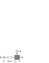
FIG. 5.: Equivalent circuit of a dot coupled to the enviroment. The grey square represents a dot, $C$ being its self capacitance; $C_{G}$– the mutual capacitnce to the environment; $Z(\omega)$– the linear impedance of the environment. Here $U$ represents the noise voltage. The black arrow is a tunneling tip through which particles may be injected to the dot, measuring its DOS. This tip may be coupled to the dot through a large impedance barrier.

Phenomenologically it is convenient to consider an equivalent circuit (Fig. 5), assigning the self capacitance, $C$, (bare interaction) to the dot, which in turn is capacitively coupled (through $C_{G}$) to the gate electrode. The gate is electrically coupled to the ground through the linear impedance $Z(\omega)$. The voltage source, $U$, represents the equilibrium noise voltage of the entire circuit. We shall model the dot–environment interaction by assuming that the dot is subjected to a time dependent (but spatially uniform) noise potential due to the environment

$$H_{noise}=\eta(t)\sum_{\alpha}a^{+}_{\alpha}a_{\alpha}.$$ (32)

At the end of these calculations all physical quantities should be averaged over realizations of the noise. We shall assume further that the noise is Gaussian with zero mean value. The averaging procedure thus may be written as

$$\langle\ldots\rangle_{noise}=\frac{1}{{\cal N}}\int{\cal D}[\eta(\tau)]e^{-\frac{1}{2}\int\int_{0}^{\beta}d\tau d\tau^{\prime}\eta(\tau)K^{-1}(\tau-\tau^{\prime})\eta(\tau^{\prime})}\ldots\,\,,$$ (33)

where ${\cal N}$ is a normalization factor and $K(\tau-\tau^{\prime})=\langle\eta(\tau)\eta(\tau^{\prime})\rangle$ is the noise correlator, which is to be determined employing the fluctuation–dissipation theorem (FDT). An important observation is that the partition function of the dot, $Z(\mu)$, is not affected by the noise term. Indeed, we have already seen, Eq. (17), that the partition function of the electron gas in a spatially uniform a.c. field depends on its mean value only (which is zero in our case). This can be understood as a consequence of the gauge invariance of the partition function – spatially uniform field may be always removed by a gauge transformation. As a result, the noise term in Eq. (12) enters in the numerator only. Averaging Eq. (12) over the Gaussian noise, Eq. (33), leads to an effective fermionic action with interaction which is non–local in time,

$$S_{int}[\psi^{*}_{\alpha},\psi_{\alpha}]=\frac{1}{2}\int\!\!\!\int_{0}^{\beta}d\tau d\tau^{\prime}\sum_{\alpha}\psi^{*}_{\alpha}(\tau)\psi_{\alpha}(\tau)\left(V^{[0]}\delta(\tau-\tau^{\prime})-K(\tau-\tau^{\prime})\right)\sum_{\alpha}\psi^{*}_{\alpha}(\tau^{\prime})\psi_{\alpha}(\tau^{\prime}).$$ (34)

As a result, one obtains an effective renormalization (screening) of the zero–mode interaction potential

$$V^{[0]}\rightarrow V(\omega_{m})=V^{[0]}-K(\omega_{m}).$$ (35)

Further calculations follow the same steps outlined in Sec. II. The final result is given again by Eq. (23) where now (cf. Eq. (24))

$$S(\tau)=T\sum_{m\neq 0}\frac{V(\omega_{m})}{\omega_{m}^{2}}(1-e^{i\omega_{m}\tau}).$$ (36)

We shall next employ the FDT to calculate the noise correlator, $K(i\omega)$. According to the FDT the equilibrium noise spectrum ($T=0$) of the total noise voltage generated by the circuit is $\langle UU\rangle=e^{2}i\omega Z_{tot}$, where the total impedance of the equivalent circuit is $Z_{tot}=(i\omega C)^{-1}+(i\omega C_{G})^{-1}+Z(\omega)$. The corresponding voltage drop on the dot is $\eta=U(i\omega C)^{-1}/Z_{tot}$; thus the noise correlator, $K=\langle\eta\eta\rangle$, is given by

$$K(i\omega)=\frac{e^{2}}{C}\frac{1/(i\omega C)}{Z_{tot}}.$$ (37)

Substituting this expression in Eq. (35) and rewriting it in a finite temperature form one obtains

$$V(\omega_{m})=\frac{e^{2}}{C}\,\,\frac{C/C_{G}+|\omega_{m}|ZC}{1+C/C_{G}+|\omega_{m}|ZC}.$$ (38)

The high frequency (unscreened) value coincides with that of Eq. (8), whereas at low frequency the interaction is partially screened and is given by the total capacitance, $V(0)=e^{2}/(C+C_{G})$. The characteristic crossover frequency is given by the “$RC$” time of the circuit, $\omega\approx(ZC)^{-1}$. As a result the long time behavior of $S(\tau)$, determined by the small frequency asymptotic of the screened interaction, is given by $S(\tau)\approx|\tau|e^{2}/2(C+C_{G})$ for $ZC\ll\tau\ll\beta$.

A case of particular interest is that of a “maximally” screened interaction, when $V(i\omega\rightarrow 0)=0$. In this case the linear term in $S(\tau)$ is absent and the action grows at most logarithmically at large $\tau$. This would immediately imply that instead of exponential suppression of the DOS at the Fermi energy, one obtains only a power–law ZBA. According to Eq. (38) such a case may be realized when $C_{G}\rightarrow\infty$ (more precisely $ZC_{G}\gg\beta$). This is the case of a dot strongly connected to the environment. For simplicity we restrict ourselves to the scenario of a pure ohmic environment, $Z=R$, in which case the interaction potential is given by [17]

$$V(\omega_{m})=V^{[0]}\,\frac{|\omega_{m}|}{\Omega+|\omega_{m}|},$$ (39)

where $\Omega\equiv(RC)^{-1}$ and $V^{[0]}$ is given by Eq. (8). As $V(\omega=0)=0$ the addition or subtraction of an electron from the dot costs no Coulomb energy over long time scales. On short time scales, however, before the environment adjusts to screen out the added electron, one has to pay some energy, Eq. (39). Thus the addition of an electron can be considered as “tunneling” under an energy barrier in the time direction. The very same physics has been discussed in the context of $d=2$ systems in Refs. [18, 6]. The related energy cost on short time scales suppresses free particle exchange between the dot and the particle reservoir (although Coulomb blockade in its strict sense is absent). This leads to the suppression of the tunneling DOS hence to ZBA. Substituting Eq. (39) into Eq. (36), one obtains for $\Omega^{-1}\ll\tau\ll\beta$ [19]

$$S(\tau)\approx 2r\log(1+\tilde{\Omega}|\tau|)+O\left((\Omega\tau)^{-1}\right)\,,$$ (40)

where $\tilde{\Omega}\equiv e^{\gamma}\Omega$ with $\gamma=0.577\ldots$ being the Euler constant and $r\equiv V^{[0]}/(2\pi\Omega)=Re^{2}/(2\pi\hbar)$ is dimensionless resistance of the environment. Performing the Fourier transform and analytical continuation (see Appendix A), one obtains for the zero–temperature spectral density of the Coulomb boson

$$B(\omega)=-\frac{\mbox{sign}\,\omega}{\tilde{\Omega}}\,\frac{2\pi}{\Gamma(2r)}\left|\frac{\omega}{\tilde{\Omega}}\right|^{2r-1}e^{-|\omega/\tilde{\Omega}|}.$$ (41)

Finally the zero temperature DOS may be found from Eq. (28) with $B(\omega)$ given by Eq. (41). Assuming a constant bare DOS (i.e. $\nu^{[0]}=\mbox{const}$) one obtains

$$\frac{\nu_{0}(\epsilon)}{\nu^{[0]}}=1-\Gamma\left(2r,\left|\frac{\epsilon}{\tilde{\Omega}}\right|\right)\approx\left\{\begin{array}[]{ll}{\displaystyle\frac{1}{\Gamma(2r+1)}\left|\frac{\epsilon}{\tilde{\Omega}}\right|^{2r}};&|\epsilon|\ll\Omega,\\ {\displaystyle 1-\left|\frac{\epsilon}{\tilde{\Omega}}\right|^{2r-1}e^{-|\epsilon/\tilde{\Omega}|}};&|\epsilon|\gg\mbox{max}\{\Omega,V^{[0]}\},\end{array}\right.$$ (42)

where $\Gamma(2r,x)$ is the incomplete gamma function. For the maximally screened zero–mode interaction scenario the ZBA in $d=0$ has a power law behavior, rather than the gap given by Eq. (31). For high–impedance (slow) environment, $r\gg 1$, there is a crossover to the “orthodox” Coulomb blockade in the interval $\Omega<\epsilon<V^{[0]}$. However for the low–impedance, $r<1$, environment the power–law ZBA, Eq. (42), directly crosses over to the finite dimensional AA result at $\epsilon\approx\Omega$.

The straightforward finite temperature generalization of Eq. (41) is (see Appendix A)

$$B(\omega)=-\frac{\mbox{sinh}\,\omega/2T}{\tilde{\Omega}}\,\frac{2}{\Gamma(2r)}\left(\frac{2\pi T}{\tilde{\Omega}}\right)^{2r-1}\left|\Gamma\left(r+\frac{i\omega}{2\pi T}\right)\right|^{2}.$$ (43)

Substituting this result into Eq. (28) one obtains e.g. for the DOS at the Fermi energy, $\epsilon=0;\,\,\,T\ll\Omega$

$$\frac{\nu_{0}}{\nu^{[0]}}=a(r)\left(\frac{2\pi T}{\tilde{\Omega}}\right)^{2r},$$ (44)

where

$$a(r)\equiv\frac{1}{\pi\Gamma(2r)}\int_{0}^{\infty}dx\frac{\left|\Gamma(r+ix)\right|^{2}}{\mbox{cosh}\,\pi x}=\left\{\begin{array}[]{ll}1-\Psi\left(\frac{1}{2}\right)2r;&r\ll 1,\\ 2^{-2r}/\sqrt{\pi r};&r\gg 1;\end{array}\right.$$ (45)

$\sigma(1/2)=1/\pi;\,\,\,\sigma(1)=1/8$. At $T>\mbox{max}\{\Omega,V^{[0]}\}$ the DOS obeys Eq. (29). Screening of the zero mode interaction converts the exponential suppression of the DOS (cf. Eq. (30)) into the power–law, Eq. (44).

Our results in the limit of maximally screened interaction $C_{G}\rightarrow\infty$ are compatible with the results of Refs. [7, 8], where tunneling through a single tunnel junction coupled to a linear impedance was considered. This coincidence is not surprising at all; indeed a dot coupled to a circuit through large capacitance, $C_{G}$, can be viewed as an island from which charge can continuously leak out; this is practically the setup of Refs. [7, 8]. Our present analysis stresses the physics of a weakly coupled dot (with a finite $C_{G}$, Eq. (38)) and its relation to the ZBA. At $T=0$, employing the above given expressions one obtains

$$\frac{\nu_{0}(\epsilon)}{\nu^{[0]}}=\left\{\begin{array}[]{ll}0;&|\epsilon|\leq e^{2}/2(C+C_{G}),\\ 1-\Gamma\left(2\tilde{r},\frac{|\epsilon|-e^{2}/(C+C_{G})}{\tilde{\Omega}(C+C_{G})/C_{G}}\right);&e^{2}/2(C+C_{G})<|\epsilon|,\end{array}\right.$$ (46)

where $\tilde{r}\equiv r[C_{G}/(C+C_{G})]^{2}$. At finite temperature and $\epsilon=0$ one has

$$\frac{\nu_{0}}{\nu^{[0]}}\approx\left\{\begin{array}[]{ll}\exp\{-e^{2}/8T(C+C_{G})\};&T\leq e^{2}/2(C+C_{G}),\\ (T/\tilde{\Omega})^{2\tilde{r}};&e^{2}/2(C+C_{G})<T<\Omega,\\ 1-e^{2}/4TC;&\mbox{max}\{\Omega,e^{2}/2C\}<T\end{array}\right.$$ (47)

(the above expressions account for the ${\bf Q}=0$ contribution only). We stress that, our results are a particular, d=0, case of a general non–perturbative expression for the ZBA obtained by Nazarov [5] and Levitov and Shytov [6]. Our point here is that for $d=0$ case all calculations can be carried out exactly, avoiding some of the uncontrolled albeit plausible assumptions employed in Refs. [5, 6].

V Acknowledgments

We are grateful to A. Altland, M. Devoret, U. Sivan and B. Shklovskii for useful suggestions. In particular we are indebted to A. M. Finkelstein for his comments on the relation between the structure of the density of states and gauge invariance. This research was supported by the German–Israel Foundation (GIF) and the U.S.–Israel Binational Science Foundation (BSF) and the Israel Academy of Sciences.

A

This Appendix is devoted to the calculation of the spectral density of the Coulomb boson, ${\cal D}(\tau)=\exp\{-S(\tau)\}$. In the case of unscreened zero mode interaction $S(\tau)$ is given by Eq. (25). The Fourier transform has a form

$${\cal D}(\omega_{m})=\int_{0}^{\beta}d\tau e^{i\omega_{m}\tau}e^{-\frac{V^{[0]}}{2}(\tau-\beta^{-1}\tau^{2})}.$$ (A1)

Deforming the contour of integration as it shown on Fig. 6 and making the obvious redefinition of variables one obtains

$${\cal D}(\omega_{m})=i\int_{0}^{\infty}dte^{-\omega_{m}t-\frac{V^{[0]}t^{2}}{2\beta}}\left(e^{-iV^{[0]}t/2}-e^{iV^{[0]}t/2}\right).$$ (A2)

In this expression one can perform analytical continuation, resulting in ${\cal D}^{R}(\omega)={\cal D}(\omega_{m}\rightarrow-i\omega+\delta)$. The imaginary part of ${\cal D}^{R}(\omega)$ may be easily evaluated extending the region of integration up to $-\infty$. As a result, $B(\omega)=-2\Im{\cal D}^{R}(\omega)$ is given by Eq. (27).

FIG. 6.: Countour of integration in Eq. (A1).

Next we discuss the maximally screened zero mode interaction. For $0<\tau\ll\beta/2$ the action is given by Eq. (40). Periodicity and symmetry requires that for $\beta/2\ll\tau<\beta$ action has the form $S(\tau)\approx 2r\log(1+\tilde{\Omega}(\beta-\tau))$. Performing the Fourier transform by deforming the contour of integration and analytical continuation exactly as for the non–screened interaction, one obtains $B(\omega)=-F(\omega)+F(-\omega)$, where

$$F(\omega)=2\Re\int_{0}^{\infty}dt\frac{e^{i\omega t}}{(1+i\tilde{\Omega}t)^{2r}}=\frac{\theta(\omega)}{\tilde{\Omega}}\,\frac{2\pi}{\Gamma(2r)}\left(\frac{\omega}{\tilde{\Omega}}\right)^{2r-1}e^{-\omega/\tilde{\Omega}}.$$ (A3)

This leads to zero temperature expression, Eq. (41). To generalize the above expressions to finite temperatures we use the conformal transformation $\tau\rightarrow\sin\pi T\tau/(\pi T)$ (cf.Ref. [20]) yielding

$$F(\omega)\stackrel{{\scriptstyle T\ll\Omega}}{{\longrightarrow}}\,\, 2\Re\left[\frac{e^{-i\pi r}}{\tilde{\Omega}^{2r}}\int_{0}^{\infty}dte^{i\omega t}\left(\frac{\pi T}{\mbox{sinh}\,\pi Tt}\right)^{2r}\right]$$ (A5)

$$=\frac{e^{\omega/2T}}{\tilde{\Omega}}\frac{2\pi}{\Gamma(2r)}\left(\frac{2\pi T}{\tilde{\Omega}}\right)^{2r-1}\,\left|\Gamma\left(r+\frac{i\omega}{2\pi T}\right)\right|^{2}\,.$$

REFERENCES

- [1] B. L. Altshuler, and A. G. Aronov, Solid State Commun. 30, 115 (1979); B. L. Altshuler, A. G. Aronov, and P. A. Lee, Phys. Rev. Lett. 44, 1288 (1980);
- [2] B. L. Altshuler, and A. G. Aronov. In A. J. Efros and M. Pollak, editors, Electron–Electron Interaction In Disordered Systems, pp. 1–153. Elsevier Science Pub. B. V., North–Holland, 1985.
- [3] G. Schön, and A. D. Zaikin, Phys. Rep. 198, 237 (1990).
- [4] K. Mullen, Y. Gefen, and E. Ben–Jacob, Physica B 152, 172 (1988); D. V. Averin, and K. K. Likharev, in Mesoscopic Phenomena in Solid editors B. L. Altshuler, P. A. Lee, and R. A. Webb. Elsevier Science Publishers B. V., North–Holland, 1991, pp. 173–271.
- [5] Yu. V. Nazarov, Zh. Eksp. & Theor. Fiz., 96, 975 (1989); [Sov. Phys. JETP 68, 561 (1989)].
- [6] L. S. Levitov, and A. V. Shytov, (to be published).
- [7] M. H. Devoret, D. Esteve, H. Grabert, G.-L. Ingold, H. Pothier, and C. Urbina, Phys. Rev. Lett., 64, 1824 (1990).
- [8] S. M. Girvin, L. I. Glazman, M. Jonson, D. R. Penn, M. D. Stiles, Phys. Rev. Lett., 64, 3183 (1990).
- [9] We acknowledge very useful comments by M. Devoret on this point. Ref. [7] as well as his lecture notes (Les–Houches, 1994, to be published) contain much of the physics alluded to above.
- [10] K. A. Matveev, Zh. Eksp. & Theor. Fiz., 99, 1598 (1991); [Sov. Phys. JETP 72, 892 (1991)].
- [11] D. V. Averin, and Yu. V. Nazarov, Phys. Rev. Lett., 65, 2446 (1990).
- [12] This contribution is dominant only when the screening radius is much larger than the electron wavelength.
- [13] We shall not treat here the periodic structure as a function of .
- [14] J. W. Negele, and H. Orland, Quantum Many–Particle Systems, Addison–Wesley publishing company, 1988.
- [15] A. M. Finkelstein, Electron Liquid in Disordered Conductors, volume 14 of Soviet scientific reviews, editor I. M. Khalatnikov, Harwood Academic Publishers GmbH, 1990; A. M. Finkelstein, Physica B 197, 636 (1994).
- [16] A. A. Abrikosov, L. P. Gorkov, and I. E. Dzyaloshinski, Methods of Quantum Field Theory in Statistical Physics. Prentice–Hall, New Jersey 1963.
-
[17]
We note the connection to the dynamically screened interaction,
, discussed in Section II, cf. Eq. (4).
Making the extension (
being a phenomenological leakage rate of the global charge in the dot) and
taking we obtain
where and . This coincides with Eq. (39) for . - [18] B. Spivak, unpublished (1990).
- [19] Although Eq. (40) is supposed to be valid only for , it has an almost correct behavior for small as well. As one expects, the short time () behavior of the action corresponds to an unscreened interaction, cf. Eq. (25), , whereas Eq. (40) leads to . Consequently our results, based on Eq. (40) are expected to be qualitatively correct even for .
- [20] R. Shankar, Int. J. Mod. Phys. B 4, 2371 (1990); C. de C. Chamon, D. E. Freed, and X. G. Wen, Phys. Rev. B 51, 2363 (1995).