Thermodynamics of finite magnetic two-level systems

Abstract

We use Monte Carlo simulations to investigate the thermodynamical behaviour of aggregates consisting of few superparamagnetic particles in a colloidal suspension. The potential energy surface of this classical two-level system with a stable and a metastable “ring” and “chain” configuration is tunable by an external magnetic field and temperature. We determine the complex “phase diagram” of this intriguing system and analyze thermodynamically the nature of the transition between the ring and the chain “phase”.

With progressing miniaturization of devices, there is growing interest in the thermodynamical behaviour of finite-size systems [1]. A central question in this respect is, whether small systems can exhibit well-defined transitions that could be interpreted as a signature of phase transitions which, strictly speaking, are well defined only in infinite systems. So far, reproducible features of the specific heat have been interpreted as indicators of “melting” transitions in small rare gas clusters [2, 3].

Here we investigate the intriguing thermodynamical behaviour of a structurally relaxed finite system which is controlled by two external variables, namely the temperature $T$ and the magnetic field $B_{\rm ext}$. The system of interest consists of few near-spherical, superparamagnetic particles with a diameter of $\approx 10-500$ Å in a colloidal suspension. Such systems, covered by a thin surfactant layer, are readily available in macroscopic quantities, are called ferrofluids, and are known to form complex labyrinthine [4] or branched structures [5] as many particle systems, whereas the only stable states for systems with few particles ($N<14$) are the “ring” and the “chain” [6].

The existence of two environmental variables, yet still only two isomer states, gives rise to a thermodynamical behaviour of unprecedented richness, as compared to that of other small clusters, such as the noble gas clusters [2, 3]. This is also an intriguing example of a classical, externally tunable finite two-level system.

We will show that the system exhibits phase transitions between two ordered phases, one magnetic and the other one nonmagnetic, as well as phase transitions between these ordered phases and a disordered phase. Whereas the system is not susceptible to small magnetic fields, it shows a strong paramagnetic response when exposed to larger magnetic fields.

Our model system consists of six spherical magnetite particles with a diameter of $\sigma=200$ Å, mass $m=1.31{\times}10^{7}$ amu, and a large permanent magnetic moment $\mu=1.68{\times}10^{5}~{}\mu_{\rm B}$. The potential energy $E_{\rm p}$ of this system in the external field $\vec{B}_{\rm ext}$ consists of the interaction between each particle $i$ and the applied field, given by $u_{i}=-\vec{\mu}_{i}\cdot\vec{B}_{\rm ext}$, and the pair-wise interaction between the particles $i$ and $j$, given by [6]

$$u_{ij} = (\mu_{0}^{2}/r_{ij}^{3})\left[\hat{\mu}_{i}\cdot\hat{\mu}_{j}-3(\hat{\mu}_{i}\cdot\hat{r}_{ij})(\hat{\mu}_{j}\cdot\hat{r}_{ij})\right]$$ (1)

$$+ \epsilon\left[\exp\left(-\frac{r_{ij}-\sigma}{\rho}\right)-\exp\left(-\frac{r_{ij}-\sigma}{2\rho}\right)\right]\;.$$ (2)

The first term in Eq. (2) is the magnetic dipole-dipole interaction energy. The second term describes a non-magnetic interaction between the surfactant covered tops in a ferrofluid that is repulsive at short range and attractive at long range [5]. We note that the most significant part of this interaction, which we describe by a Morse-type potential with parameters $\epsilon=0.121$ eV and $\rho=2.5$ Å, is the short-range repulsion, since even at equilibrium distance the attractive part does not exceed $10\%$ of the dipole-dipole attraction.

The equilibrium structures of small clusters are either rings or chains, both of which can be easily distinguished by their different mean magnetic moment $\langle\mu\rangle$.

In the following, we present the first complete “phase diagram” of a model aggregate of magnetic tops and describe in detail how “phase transitions” occur in such a nanoscale system. Unlike in the bulk, where transitions between well-defined phases are sharp, small aggregates in a ferrofluid transform smoothly from one configuration to another due to changes in the two environmental variables $B_{\rm ext}$ and $T$. Our results presented below are based on a careful analysis of set of 32 extensive Metropolis Monte Carlo simulations [7], each of which consisting of $6{\times}10^{9}$ steps.

The canonical partition function, from which all thermodynamical quantities can be derived, is given by

$$Z(B_{\rm ext},T) = (2\pi\beta)^{-6N/2}\int\left[\prod_{i=1}^{N}{\rm d}\vec{x}_{i}\;{\rm d}\phi_{i}\;{\rm d}\theta_{i}\;{\rm d}\psi_{i}\right]$$ (3)

$$\times \exp\left(-\beta(\sum_{i<j}^{N}u_{ij}-\sum_{i}^{N}\mu_{i,\rm z}B_{\rm ext})\right)\;,$$ (4)

where $\beta=(k_{\rm B}T)^{-1}$ and where the field $\vec{B}_{\rm ext}$ is aligned with the $z$-axis. The pre-exponential factor addresses the fact that each particle has three rotational and three center-of-mass degrees of freedom. The key quantities we monitor as a function of $T$ and $B_{\rm ext}$ are the formation enthalpy $E^{*}$ of the isolated system that is decoupled from the external field, given by $E^{*}=\sum_{i<j}u_{ij}=E_{\rm p}+\mu_{z}B_{\rm ext}$, and the $z$-component of the total magnetic moment of the aggregate, $\mu_{z}$. By monitoring these two response quantities to the external temperature and field during all simulations, we determine the weighted density of states

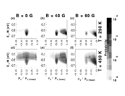
FIG. 1.: Monte Carlo results for the probability to find an aggregate in a state with its magnetic moment in the field direction $\mu_{z}$ and potential energy $E_{\rm p}$. The individual contour plots show our results for the temperature $T=250$ K at the field values (a) $B_{\rm ext}$=0 G, (b) $B_{\rm ext}$=40 G, (c) $B_{\rm ext}$=60 G, and $T=$450 K at the field values (d) $B_{\rm ext}$=0 G, (e) $B_{\rm ext}$=40 G, (f) $B_{\rm ext}$=60 G.

$$P(E^{*},\mu_{z};B_{\rm ext},T) = Z^{-1}(B_{\rm ext},T)\;\rho(E^{*},\mu_{z})\;$$ (5)

$$\times \exp(-\beta(E^{*}-\mu_{z}B_{\rm ext}))\;,$$ (6)

which gives the probability to find the system in a state with the formation enthalpy $E^{*}$ and magnetic moment $\mu_{z}$. The partition function $Z$, which appears as the normalization constant, can be rewritten as

$$Z(B_{\rm ext},T) =(2\pi\beta)^{-6N/2}$$ (8)

$$\int{\rm d}E^{*}{\rm d}\mu_{z}\;\rho(E^{*},\mu_{z})\;\exp(-\beta(E^{*}-\mu_{z}\;B_{\rm ext}))\;.$$

We then combined the results of all simulations using the optimized Monte Carlo data analysis of Ferrenberg et al. [8, 9] in order to calculate the normalized density of states ${\rho}(E^{*},\mu_{z})$ and ${\rho}(E_{p},\mu_{z})$ with minimized statistical error [10]. Using the above defined density of states, the field- and temperature dependence of the expectation value of any function $F(E^{*},\mu_{z})$ can be obtained as

$$<F(E^{*},\mu_{z};B_{\rm ext},T)>=$$ (9)

$$\int{\rm d}\mu_{z}\;\int{\rm d}E^{*}\;F(E^{*},\mu_{z})\;{P}(E^{*},\mu_{z};B_{\rm ext},T)\;.$$ (10)

For the system described here we found it imperative to perform the simulations at sufficiently high temperatures in order to cover the whole configuration space properly. At low temperatures the thermal equilibrium might not be achieved even after extremely long iteration times, since transitions between rings and chains are very infrequent and might never occur. In order to obtain a first idea about the stable and metastable states of the system, we plotted in Fig. 1 the probability $\tilde{P}(E_{\rm p},\mu_{z};B_{\rm ext},T)$ of finding the aggregate in a state with potential energy $E_{\rm p}$ and total magnetic moment in the field direction $\mu_{z}$. This is the projection of the probability to find the system in a specific state in the high-dimensional configuration space onto the $(E_{\rm p},\mu_{z})$ subspace. Regions in the $(E_{\rm p},\mu_{z})$ subspace with a high probability indicate not only the energetic preference of corresponding states, but also a large associated phase space volume.

Rings always have an absolute magnetic moment $|\mu/\mu^{\rm max}|$ that is close to zero. Consequently, also the $z$-component of the magnetic moment of rings is near zero, as seen in Fig. 1. Even though the absolute magnetic moment $|\mu/\mu^{\rm max}|$ of chains is close to one, these aggregates can not easily be distinguished from rings in the absence of a field. In zero field, chains have no orientational preference and the $z$-component of their magnetic moment, $\mu_{z}/\mu_{z}^{\rm max}$, also averages to zero. Of course, chains – unlike rings – do align with a nonzero magnetic field and, especially at low temperatures, show a magnetic moment $\mu_{z}/\mu_{z}^{\rm max}{\approx}1$ in the field direction.

The relative stability of an aggregate is reflected in its potential energy $E_{\rm p}$. We find $E_{\rm p}$ to increase (corresponding to decreasing stability) with increasing temperature. On the other hand, applying a magnetic field destabilizes rings in favour of field-aligned chains. With increasing field, chains are confined to a gradually decreasing fraction of the configurational space which sharpens their distribution in the $(E_{\rm p},\mu_{z})$ subspace, as seen when comparing Figs. 1(a)–(c) and Figs. 1(d)–(f).

Under all conditions, we find two more or less pronounced local maxima in the probability distribution $P$, corresponding to a ring with $0{\lesssim}\mu_{z}/\mu_{z}^{\rm max}{\ll}1$, and a chain with $0{\ll}\mu_{z}/\mu_{z}^{\rm max}{\lesssim}1$. At zero field we observe a predominant occupation of the more stable ring state. Due to the relatively small energy difference with respect to the less favourable chain ${\Delta}E_{\rm p}^{\rm cr}/N=(E_{\rm p}^{\rm chain}-E_{\rm p}^{\rm ring})/N=0.06$ eV, both states get more evenly occupied at higher temperatures. At fields as low as $B_{\rm ext}=40$ G, the energy difference between chains and rings drops significantly to ${\Delta}E_{\rm p}^{\rm cr}/N=0.02$ eV. As seen in Fig. 1(b), this results in an equal occupation of both states even at low temperatures. At the much higher field value $B_{\rm ext}=60$ G, chains are favoured with respect to the rings by a considerable amount of energy ${\Delta}E_{\rm p}^{\rm cr}/N=-0.2$ eV. This strongly suppresses the occurrence of rings, as seen in Figs. 1(c) and (f).

Fig. 1 shows not only the stable and metastable states under given conditions, but also the states found along the preferential transition pathway between a ring and a chain in the projected $(E_{\rm p},\mu_{z})$ subspace. During the transition between a chain and a ring, each aggregate must undergo a continuous change of $E_{\rm p}$ and $\mu_{z}$. The favoured transition pathways are then associated with high-probability trajectories in the $(E_{\rm p},\mu_{z})$ subspace. The value of the activation barrier ${\Delta}E_{\rm p}^{\rm act}$ is then given by the largest increase of $E_{\rm p}$ along the optimum transition path which connects the stable and metastable ring and chain islands. In our simulations we found that the activation barrier occurred always at $\mu_{z}/\mu_{z}^{\em max}{\approx}0.22$. Consequently, we concluded that the field dependence of the activation energy follows the expression ${\Delta}E_{\rm p}^{\rm act}(B_{\rm ext})={\Delta}E_{\rm p}^{\rm act}(B_{\rm ext}=0)-0.22\;\mu_{z}^{\rm max}\;B_{\rm ext}$.

In order to quantitatively describe the “phase transitions” occurring in this system, we focused our attention on the specific heat and the magnetic susceptibility. The specific heat per particle in a canonical ensemble is given by $c_{B}={\rm d}{\langle}E/N{\rangle}/{\rm d}T$, where the total energy is given by $E=\frac{3}{2}Nk_{\rm B}T+E_{\rm p}$. Correspondingly, we define the magnetic susceptibility per particle as $\chi={\rm d}{\langle}\mu_{z}/N{\rangle}/{\rm d}B_{\rm ext}$. These response functions are related to the fluctuations of $E_{\rm p}$ and $\mu_{z}$ by

$$c_{B} = \left[\frac{6N}{2}k_{\rm B}+k_{\rm B}\beta^{2}(\langle E^{2}\rangle-\langle E\rangle^{2})\right]/N\;,$$ (11)

$$\chi = \left[\beta(\langle\mu_{z}^{2}\rangle-\langle\mu_{z}\rangle^{2})\right]/N\;.$$ (12)

Phase transitions are only well-defined in infinite systems and are associated with a discontinuous change in the total energy and specific heat when crossing the phase boundary. The corresponding changes in finite systems are more gradual. This is seen in the well defined, yet not sharp “crest line” separating the ring and the chain “phase” in the $T-B_{\rm ext}$ “phase diagram” in Fig. 2(a). These results illustrate how the critical magnetic field for the ring-chain transition decreases with increasing temperature. At high temperatures, the “line” separating the “phases” broadens significantly into a region where rings and chains coexist.

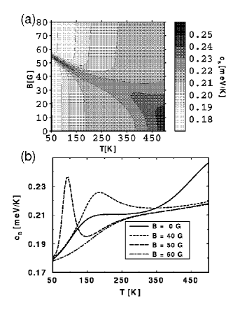
FIG. 2.: Specific heat per particle $c_{B}$ of the system as a function of temperature $T$ and the external magnetic field $B_{\rm ext}$. Results for the entire temperature and field range investigated here are presented as a contour plot in (a). The temperature dependence of $c_{B}$ for selected values of $B_{\rm ext}$ is presented in (b).

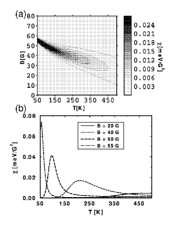
FIG. 3.: Magnetic susceptibility per particle $\chi$ of the system as a function of temperature $T$ and the external magnetic field $B_{\rm ext}$. Results for the entire temperature and field range investigated here are presented as a contour plot in (a). The temperature dependence of $\chi$ for selected values of $B_{\rm ext}$ is presented in (b).

The line plot in Fig. 2(b) is the respective constant-field cut through the contour plot in Fig. 2(a). As can be seen in Fig. 2(b), there is no transition from chains to rings, indicated by a peak in $c_{B}$, at fields exceeding $50$ G, which is close to the critical field value at which chains become favoured over rings at zero temperature. At fields $B_{\rm ext}<<40$ G, on the other hand, there is no region where chains would be thermodynamically preferred over the rings, and we only observe a gradual transition from the ring phase into the coexistence region with increasing temperature. The specific heat behaviour at zero field resembles that of a small system with a gradual melting transition close to $150$ K and an onset of disorder at about $350$ K [11]. As seen in Fig. 2(b), the critical temperature and the width of the transition region can be externally tuned by the second thermodynamical variable, the external magnetic field $B_{\rm ext}$.

Fig. 3 displays the magnetic susceptibility $\chi$, another prominent indicator of phase transitions in magnetic systems, as a function of T and $B_{\rm ext}$. Like the specific heat in Fig. 2(a), the crest line in $\chi$ separates the chain “phase” from the ring “phase” in this $T-B_{\rm ext}$ “phase diagram”. Moreover, Fig. 3 reveals the fundamentally different magnetic character of these “phases”. Whereas the system is nonmagnetic in the ring “phase” found below $40$ G, it behaves like a ferromagnet consisting of Langevin paramagnets in the chain “phase” at higher fields. The transition between these states is again gradual, as expected for finite systems. The line plot in Fig. 3(b) is the respective constant-field cut through the contour plot in Fig. 3(a). When the system is in the chain “phase” it behaves like a paramagnet obeying the Curie-Weiss law, as can be seen in Fig. 3(b)[12].

At relatively low temperatures, where the aggregates are intact, the expectation value of the magnetic moment first increases due to the gradual conversion from nonmagnetic rings to paramagnetic chains. According to Fig. 3(b), this uncommon behaviour persists up to $T=200$ K at B${}_{\rm ext}=40$ G. This trend is reversed at higher temperatures, where all aggregates eventually fragment into single paramagnetic tops. In this temperature range, the magnetic moment as well as the susceptibility decreases with increasing temperature.

Since the transition probability between both states is extremely low at low temperatures and fields, magnetically distinguishable metastable states can be frozen in. A chain configuration, which is metastable in zero field, can be prepared by first annealing the system to $T{\gtrsim}350$ K and subsequent quenching in a strong field. Similarly, a frozen-in ring configuration is unlikely to transform to a chain at low temperatures, unless exposed to very large fields. Thus the above described phase diagrams can be used to externally manipulate the self-assembly of magnetic nanostructures.

In conclusion we have studied the thermodynamical behaviour of a finite two-level system, which is externally tunable by two independent variables, namely the temperature and the magnetic field. Much of the behaviour encountered in this system, such as transitions between different states, has a well-defined counterpart in infinite systems. The reason for the encountered richness of the thermodynamic and magnetic properties is the relative ease of structural transformations, which is typical for finite systems. Consequently, we expect other finite magnetic systems, e.g. small transition metal clusters, where a small number of structural isomers with substantially different magnetic moments could coexist [13], to follow this behaviour. Moreover, we expect that our results can also be transferred to nanocrystalline material, such as magnetic clusters encapsulated in the supercages of zeolites, which will likely retain some of the intriguing properties of the isolated finite systems.

DT, PJ and SGK acknowledge financial support by the NSF under Grant No. PHY-92-24745 and the ONR under Grant No. N00014-90-J-1396.

REFERENCES

- [1] Kaigham S. Gabriel, Scientific American 273(3), 150 (1995).
- [2] Ralph E. Kunz and R. Stephen Berry, Phys. Rev. Lett. 71, 3987 (1993); David J. Wales and R. Stephen Berry, Phys. Rev. Lett. 73, 2875 (1994).
- [3] P. Borrmann, COMMAT 2, 593 (1994); G. Franke, E.R. Hilf, P. Borrmann, J. Chem. Phys. 98, 3496 (1993).
- [4] Akiva J. Dickstein, et.al. Science 261, 1012 (1993).
- [5] Hao Wang, Yun Zhu, C. Boyd, Weili Luo, A. Cebers and R.E. Rosensweig, Phys. Rev. Lett. 72, 1929 (1994).
- [6] P. Jund, S.G. Kim, D. Tománek, and J. Hetherington, Phys. Rev. Lett. 74, 3049 (1995).
- [7] N. Metropolis, A. Rosenbluth, M.N. Rosenbluth, A.H. Teller, E. Teller, J. Chem. Phys. 21, 1087 (1953).
- [8] A.M. Ferrenberg, R.H. Swendsen, Phys. Rev. Lett. 61, 2635 (1988).
- [9] A.M. Ferrenberg, R.H. Swendsen, Phys. Rev. Lett. 63, 1195 (1989).
- [10] We extended the Ferrenberg analysis in a straight-forward way to deal with a two-dimensional density of states.
- [11] R. S. Berry, J. Jellinek,G. Natanson, Chem. Phys. Lett. 107, 227 (1984); G. Natanson, F. Amar, R. S. Berry, J. Chem. Phys. 78, 399 (1983).
- [12] Our numerical approach did not allow to investigate the temperature region below K. The onset of the Curie-Weiss behaviour, indicated by a maximum in at nonzero temperature, can be seen whenever the system is in the chain “phase”.
- [13] P. Borrmann, B. Diekmann, E.R. Hilf, D. Tománek, Surface Review and Letters (1996).