Glassy Vortex State in a Two-Dimensional Disordered XY-Model

Abstract

The two-dimensional XY-model with random phase-shifts on bonds is studied. The analysis is based on a renormalization group for the replicated system. The model is shown to have an ordered phase with quasi long-range order. This ordered phase consists of a glass-like region at lower temperatures and of a non-glassy region at higher temperatures. The transition from the disordered phase into the ordered phase is not reentrant and is of a new universality class at zero temperature. In contrast to previous approaches the disorder strength is found to be renormalized to larger values. Several correlation functions are calculated for the ordered phase. They allow to identify not only the transition into the glassy phase but also an additional crossover line, where the disconnected vortex correlation changes its behavior on large scales non-analytically. The renormalization group approach yields the glassy features without a breaking of replica symmetry.

I Introduction

The two-dimensional XY-model with random phase-shift, defined in Eq. (1) below, captures the physics of a variety of physical systems. Among them are XY-magnets with non-magnetic impurities, which are coupled to the XY-spins via the Dzyaloshinskii-Moriya interaction,[1] Josephson-junction arrays with geometric disorder,[2] and crystals with quenched impurities.[3] Disordered XY-models are related to even more physical systems, like impure superconductors. It is in particular the interest in vortex-glass phases in type-II superconductors, which motivates an analysis of possible glassy features in the paradigmatic two-dimensional bond-disordered system.

The most fundamental question is, whether this model has an ordered phase. In the absence of disorder, there exists at low temperatures a phase with quasi long-range order. The famous Kosterlitz-Thouless transition separates it from the high-temperature phase with short-ranged order.[4, 5] The analysis by Cardy and Ostlund[6] and more explicitly by Rubinstein, Shraiman and Nelson[1] predicted that the phase transition should be reentrant in the presence of disorder. Later Korshunov suggested,[7] that the ordered phase might be completely destroyed by disorder. Ozeki and Nishimori[8] showed for models with gauge-invariant disorder distributions, that the phase transition cannot be reentrant, leaving open whether the ordered phase does exist or not. Experiments[9] on Josephson junction arrays and simulations[10] were in favor of the existence of an ordered phase without reentrance.

In this controversial situation Nattermann, Scheidl, Korshunov, and Li[11] as well as Cha and Fertig[12] reconsidered only recently the problem and found that the ordered phase does exist and its boundary does not have reentrant shape. The earlier observation of reentrance was attributed to an overestimation of vortex fluctuations at low temperatures.

The present study extends Refs. [11] and [12], which focused on the absence of reentrance. The purpose of this article is to examine in more detail the ordered phase, which is shown to be composed of different regions. They are distinguished by the behavior of vortex correlation functions on large length scales, which are calculated quantitatively. A low-temperature regime is found to exhibit glassy behavior in its correlations.

In addition to the previous studies we find that the strength of disorder is increased under renormalization. This effect does not destroy the ordered phase but it is crucial for the universality type of the transition at low temperatures.

In the following a generalized self-consistent screening approach is applied to the replicated system. The main improvement compared to earlier approaches[1, 6, 7] on the same basis is achieved by including all relevant fluctuations and by taking special care when the number of replicas is sent to zero.

We use the replica formalism mainly for two reasons: i) The calculation of correlations becomes very convenient: one may use an expansion technique (small fugacity and density of vortices) which fails[11, 12, 13] in the unreplicated system. ii) We show that in the present model there is no need for replica symmetry breaking, even at lowest temperatures. In particular, the reentrance disappears and the glassiness occurs without a breaking of replica symmetry. This might astonish, since for various disordered systems reentrance has been explained as an artifact of a replica-symmetric (exact mean-field or approximate variational) approach, which has been overcome by breaking the replica symmetry.[14]

The paper is organized as follows: In Sec. II we set up our model and map it onto an effective Coulomb gas. We recapitulate the breakdown of fugacity expansion in the presence of disorder. In Sec. III we set up the renormalization group within a self-consistent formulation of screening. The consistency of this approach in the original and replicated system is demonstrated. Sec. IV is devoted to the evaluation of the self-consistency and the proper performance of the replica limit. The results of the renormalization group treatment are worked out in Sec. V, which are discussed and compared to the results of previous work in Sec. VI.

II The Model

The XY-model with random phase-shifts is given by the reduced Hamiltonian

$${\cal H}=-K\sum_{<{\bf r,r}^{\prime}>}\cos(\theta_{\bf r}-\theta_{\bf r^{\prime}}-A_{<{\bf r,r}^{\prime}>}).$$ (1)

It refers to a square lattice with unit spacing in two dimensions. An XY-spin with angle $\theta_{\bf r}\in[-\pi,\pi[$ is attached to every lattice site (position ${\bf r}$). The reduced spin coupling between nearest neighbors $<{\bf r,r}^{\prime}>$ reads $K=J/T$. The interaction involves quenched random phase-shifts with variance $\overline{A_{<{\bf r,r}^{\prime}>}^{2}}=\sigma$, which are uncorrelated on different bonds. Thermal fluctuations are weighted according to the partition sum

$$Z=\int_{-\pi}^{\pi}{\cal D}\{\theta\}\ e^{-{\cal H}}.$$ (2)

This XY-model can be mapped approximately onto an effective Coulomb gas. Since this procedure is well known in the absence of disorder[15, 16] and can be performed similarly in the presence of disorder, we recall only briefly the main manipulations leading to the effective model. In order to simplify the analysis of model (2), one can replace approximately the cosine-interaction by the Villain-interaction.[15] Thereby an additional variable, the vortex density $N$ is introduced. The decisive advantage of this approximation is, that the Hamiltonian becomes bilinear in the angles. All configurations of the original angles can be expressed in terms of spin-waves and vortices. Just as in the pure case, spin-waves and vortices decouple energetically. Since spin-waves are simply harmonic, all non-trivial physics arises from vortices with an effective Hamiltonian

$${\cal H}_{\rm v} = \int_{\bf k}\frac{2\pi^{2}K}{k^{2}}\left|N_{\bf k}-Q_{\bf k}\right|^{2}$$ (4)

$$= E\sum_{\bf R}(N_{\bf R}-Q_{\bf R})^{2}-$$ (6)

$$-\sum_{\bf R\neq R^{\prime}}\pi K\ln|{\bf R}-{\bf R}^{\prime}|(N_{\bf R}-Q_{\bf R})(N_{\bf R^{\prime}}-Q_{\bf R^{\prime}}),$$

in Fourier and real space, and the partition sum

$$Z_{\rm v}=\sum_{\{N\}}e^{-{\cal H}_{\rm v}}.$$ (7)

Here $N_{\bf R}$ is the integer-valued vortex density, which is subject to thermal fluctuations. On the square lattice $N_{\bf R}$ is associated with plaquettes (dual sites), which are labeled by ${\bf R}$ in contrast to sites ${\bf r}$. Thermal vortices $N$ couple to a background of quenched vortices $Q_{\bf R}=\frac{1}{2\pi}{\nabla}\times{\bf A}$. The last expression means, that the plaquette variable $Q_{\bf R}$ is given by the rotation of variable $A$ on the surrounding bonds. From this relation one immediately derives, that the quenched vortices are Gaussian random variables with variance $\overline{Q_{-\bf k}Q_{\bf k}}=\frac{\sigma}{4\pi^{2}}k^{2}$. A single phase-shift $A_{<{\bf r,r}^{\prime}>}$ creates a dipole of quenched vortices situated in the plaquettes which have the bond $<{\bf r},{\bf r}^{\prime}>$ as side. Therefore quenched vortices are anti-correlated and their total vorticity vanishes.

We recognize from Eq. (4), that only neutral configurations of vortices will have finite energy. Hence the partition sum can be restricted to neutral configurations (i.e. $\sum_{\bf R}{\bf N}_{\bf R}=0$) like in the pure case. Every such neutral configuration can be imagined as a superposition of dipoles of a vortex ($N=1$) and an antivortex ($N=-1$). In analogy to electrostatics, vortices of the same sign repel each other and vortices of different sign attract each other.

Since the interaction is logarithmic, vortices build a Coulomb gas. The interaction is identical among the thermal and quenched component. The Fourier representation (4) of the vortex Hamiltonian makes evident, that thermal vortices try to compensate quenched vortices as well as possible. A perfect compensation is prevented by the fact, that $N_{\bf R}$ is restricted to integer values, whereas $Q_{\bf R}$ is a continuous random variable.

In Eq. (6) we introduced the vortex core energy $E=\pi\gamma K$, where $\gamma$ takes the value $\gamma\approx 1.6$ on a square lattice. It emerges from the lattice Greens function [cf. Eq. (4.13a) of Ref. [16]]. Although $\gamma$ has a unique value for the lattice model, it will occasionally be considered as an independent parameter which allows to control the density of vortices irrespectively of $K$. In a dilute vortex system with $N_{\bf R}=0,\pm 1$ only, $E$ is comparable to a chemical potential.

In a region of parameters, where vortices are negligible, fluctuations of the original angle variables are given only by spin waves. They lead to a decay of the spin correlation function[1, 6]

$$\Gamma({\bf r})=\overline{\langle\cos[\theta({\bf r})-\theta({\bf 0})]\rangle}\sim r^{-\eta}$$ (8)

with exponent $\eta={(1/K+\sigma)/2\pi}$. If the correlation decays algebraically even in the presence of vortices, the system has quasi long-range order.

As vortices are excited thermally, they give rise to additional fluctuations in the angles, the correlation will decay faster. This effect can be expressed by a renormalized $\eta$, which becomes scale dependent. If vortices lead to a divergence of the renormalized $\eta$ on large scales, quasi long-range order is destroyed. However, vortex fluctuations are not only responsible for such a quantitative effect, they also drive the phase transition into the high-temperature phase, where the spin-spin correlation decays exponentially.[4]

Let us estimate, to what extent disorder can favor the excitation of vortices. In the pure case $Q=0$, the ground state of (4) is vortex-free. The density of vortices vanishes for vanishing temperature, since the creation of quantized vortices always costs finite energy. Therefore the pure system has a phase with quasi long-range order (8) at low temperatures.

A simple argument shows, that the disordered system has even at zero temperature a finite density of vortices:[11, 12] we consider two positions at distance $R$ and determine the probability of finding there a vortex-antivortex pair. The energy of such a dipole is given by $U_{\rm dipole}(R)\approx 2\pi J\ln R$, where we neglect the core energy for large $R$. Disorder gives and additional energy contribution $V_{\rm dipole}(R)$. At $T=0$, the dipole will be present, if its total energy $U_{\rm dipole}(R)+V_{\rm dipole}(R)$ is negative. The original Gaussian distribution of the random phase-shifts results in a Gaussian distribution of $V_{\rm dipole}(R)$ with variance $\Delta^{2}(R):=\overline{V_{\rm dipole}^{2}(R)}\approx 4\pi\sigma J^{2}\ln R$. Thus the probability

$$P(R) = \int_{-\infty}^{-U_{\rm dipole}(R)}\frac{dV}{\sqrt{2\pi\Delta(R)}}\ e^{-V^{2}/2\Delta^{2}(R)}$$ (9)

$$\approx \sqrt{\frac{\sigma}{2\pi^{2}\ln R}}\ R^{-\pi/2\sigma}$$ (10)

of finding a pair at $T=0$ is finite. In other words, this shows that in the presence of disorder the ground state is no longer vortex-free and that renormalization effects can be important even at arbitrarily small temperatures.

III Screening

The goal of the present work is therefore a calculation of such renormalization effects in the presence of random phase-shifts. We use the conceptual most simple approach, a self-consistent linear response approach. For the pure Coulomb gas, this approach is equivalent[17] to the real-space renormalization group of Kosterlitz.[5] We have checked that this equivalence still holds in the presence of disorder.

We now define vortex renormalization effects by macroscopic properties of our system. As a probe we introduce additional test vortices into the system. They experience a screened interaction and the screened background potential acting on them. Let us denote the unscreened interaction between vortices $U_{\bf k}=4\pi^{2}K\frac{1}{k^{2}}$. Due to quenched disorder vortices $Q$, thermal vortices $N$ are subject to a Gaussian background potential $V_{\bf k}=U_{\bf k}Q_{\bf k}$ with variance $\overline{V_{-\bf k}V_{\bf k}}=4\pi^{2}\sigma K^{2}\frac{1}{k^{2}}$. The screened background potential and interaction are identified from the contributions to the free energy of test vortices, which are of first and second order in their vorticity[18] (see also Appendix A for some intermediate steps)

$$V_{\bf k}^{\rm scr} = U_{\bf k}(Q_{\bf k}-\langle N_{\bf k}\rangle),$$ (12)

$$U_{\bf k}^{\rm scr} = U_{\bf k}-U_{\bf k}^{2}C_{\rm con}({\bf k}).$$ (13)

It is convenient to introduce the ordinary, disconnected, and connected correlation,

$$C({\bf R}) := \overline{\langle N_{\bf R}N_{\bf 0}\rangle},$$ (15)

$$C_{\rm dis}({\bf R}) := \overline{\langle N_{\bf R}\rangle\langle N_{\bf 0}\rangle},$$ (16)

$$C_{\rm con}({\bf R}) := C({\bf R})-C_{\rm dis}({\bf R}).$$ (17)

For a specific realization of disorder, the screened interaction in principle depends explicitly on the coordinates of both interacting vortices, it is not translation invariant. Although we should in principle consider screening in the particular disorder environment, we approximately evaluate only the average screening effect by taking the disorder average, which restores the translation symmetry of the interaction.

From the large-scale behavior of the screened interaction and the variance of the screened potential one can then identify screened parameters $K^{\rm scr}$ and $\sigma^{\rm scr}$ as (for the precise definition see Appendix A)

$$K^{\rm scr} = K+2\pi^{3}K^{2}\int_{1}^{\infty}dRR^{3}C_{\rm con}(R),$$ (19)

$$\sigma^{\rm scr}(K^{\rm scr})^{2} = \sigma K^{2}-2\pi^{3}K^{2}\int_{1}^{\infty}dRR^{3}C_{\rm dis}(R)+$$ (21)

$$+4\pi^{4}\sigma K^{3}\int_{1}^{\infty}dRR^{3}C_{\rm con}(R).$$

Although we do not yet know the correlation functions, we may establish from these expressions criteria for the existence of an ordered phase. In this phase, we expect vortices to give rise only to finite screening effects, i.e. the screened parameters must have finite values. This requires $\lim_{R\to\infty}R^{4}C_{\rm con}(R)<\infty$ and a similar condition for the disconnected correlation.

In the limit of large core energy, one can calculate the correlations to leading order by considering only a single vortex dipole. In th absence of disorder, one finds $C_{\rm con}({\bf R})=C({\bf R})\sim R^{-2\pi K}$ and $C_{\rm dis}({\bf R})=0$. The condition for the ordered phase then simply reads $K\geq 2/\pi$, in agreement with the condition that the free energy a single vortex has to be positive.[4] A similar argument can be constructed for the disordered system at $T=0$, where one can estimate $C(R)\sim p(R)\sim R^{-\pi/2\sigma}$ using Eq. (9). Then the condition for order reads $\sigma\leq\pi/8$. This argument already disproves previous predictions,[1, 6, 7] that infinitesimal $\sigma>0$ would destroy order at $T=0$.

For finite core energy, screening effects have to be taken into account quantitatively for the calculation of the correlations. For this purpose we develop a self-consistent scheme in analogy to the pure case.[4, 18] We introduce scale-dependent variables $K\equiv K(l)$ and $\sigma\equiv\sigma(l)$, which include screening by dipoles of radius $1\leq R<e^{l}$ only. Then Eq. (III) can be cast in differential form:

$$\frac{d}{dl}K^{-1} = -2\pi^{3}e^{4l}C_{\rm con}(R=e^{l}),$$ (23)

$$\frac{d}{dl}\sigma = -2\pi^{3}e^{4l}C_{\rm dis}(R=e^{l}).$$ (24)

Both equations combine to a simple flow equation of the spin-spin correlation exponent, $\frac{d}{dl}\eta=-\pi^{2}e^{4l}C(R=e^{l})$.

Eqs. (III) suggests a simple “two-component picture” illustrating the screening effects of vortices. This picture virtually separates dipoles of thermal vortices $N$ into a frozen and a polarizable component. The frozen component gives rise to the $C_{\rm dis}$. It is not polarizable and does not contribute to screening of the interaction. However, since it is frozen, it behaves like the quenched disorder background and leads to an effective disorder strength represented by the screened $\sigma$. The polarizable component is the source of $C_{\rm con}$ and leads to the screening of $K$. Both components contribute equally to a renormalization of the spin exponent. This virtual separation into two components must not be taken literally. It is impossible to assign a particular dipole uniquely to one of the two components. The two-component picture is analogous to the two-fluid model of superfluidity, which also must not be taken literally in the sense that a particular atom would be either superfluid or normalfluid.

In order to take advantage from the differential screening equations, we will calculate the correlations at $R=e^{l}$ in a self-consistent way which includes screening effects by smaller dipoles. At each differential step we will also perform a simultaneous rescaling $R\to e^{-dl}R$. Then we can interpret the differential equations as renormalization group flow equations.

For the further investigation of the model, we apply the standard replica technique[19] to the partition function (7). We are going to rewrite screening in the replicated system in order to expose the consistency between screening in the unreplicated and replicated system.

The Coulomb gas (6) is replicated $n$ times and after disorder averaging one obtains the effective Hamiltonian

$${\cal H}_{n} = \sum_{\bf R}\sum_{ab}E^{ab}N_{\bf R}^{a}N_{\bf R}^{b}-$$ (26)

$$-\frac{1}{2}\sum_{{\bf R}\neq{\bf R}^{\prime}}\sum_{a,b}2\pi K^{ab}\ln|{\bf R}-{\bf R}^{\prime}|N_{\bf R}^{a}N_{\bf R^{\prime}}^{b}\ .$$

We introduce the couplings $K^{ab}=K\delta^{ab}-\hat{K}$, $\hat{K}=\sigma K^{2}/({1+n\sigma K})$ and the core energy $E^{ab}=\pi\gamma K^{ab}=E\delta^{ab}-\hat{E}$, where $E=\pi\gamma K$ and $\hat{E}=\pi\gamma\hat{K}$. On the partition sum the neutrality condition

$$\sum_{\bf R}{\bf N}_{\bf R}^{a}=0$$ (27)

is imposed for every replica.

In the replicated system, screening effects can be calculated in the same linear response scheme as before. The leading term of the free energy of test replica-vortices is of second order in the infinitesimal test vorticity. From this order, we derive a differential screening

$$\frac{d}{dl}K^{ab}=2\pi^{3}e^{4l}\sum_{cd}K^{ac}C^{cd}(R=e^{l})K^{db}$$ (28)

in analogy to Eq. (III). We introduced the replica correlation $C^{ab}(R):=\langle N^{a}_{\bf R}N^{b}_{\bf 0}\rangle_{n}$, where $\langle\dots\rangle_{n}$ denotes a thermal average in the replicated system. Since the initial interactions are replica-symmetric, i.e. the coupling has the form $K^{ab}=K\delta^{ab}-\hat{K}$, we use the replica symmetric ansatz $C^{ab}=C_{\rm con}^{(n)}\delta^{ab}+C^{(n)}_{\rm dis}$ for correlations. The relation to the correlations in the unreplicated system is provided by

$$C_{X}({\bf R})=\lim_{n\to 0}C^{(n)}_{X}({\bf R})$$ (29)

for all three types $X$ (ordinary, disconnected, and connected) of correlations, if we identify $C^{(n)}({\bf R}):=C^{aa}({\bf R})$ consistently.

Exploiting the replica symmetry of correlations, Eq. (28) decays into flow equations for $K$ and of $\hat{K}$, which read in terms of $K$ and $\sigma=\hat{K}/(K^{2}-nK\hat{K})$:

$$\frac{d}{dl}K^{-1} = 4\pi^{3}y_{\rm con}^{2},$$ (31)

$$\frac{d}{dl}\sigma = 4\pi^{3}y_{\rm dis}^{2}.$$ (32)

In order to approach the usual notation of renormalization groups, we define effective fugacities

$$y^{2}_{X}\equiv y^{2}_{X}(l):=-\frac{1}{2}e^{4l}C^{(n)}_{X}(R=1)$$ (33)

again for all three types of rescaled correlations. They are related by $y^{2}=y_{\rm dis}^{2}+y_{\rm con}^{2}$. In these definitions we took already account of rescaling of lengths, which generates an additional flow of the core energies,

$$\frac{d}{dl}E = \pi K,$$ (35)

$$\frac{d}{dl}\hat{E} = \pi\hat{K}.$$ (36)

Eqs. (III) together with (33) constitute the main renormalization group flow equations. From relations (29) we recognize, that the flow equations of $K$ and $\sigma$ of the unreplicated system coincide with those of the replicated system in the limit $n\to 0$. In the next section these equations will be completed by a flow equation of the free energy, which however does not feed into the other flow equations.

IV Self-consistent closure

The flow equations (III) together with (33) can not yet be evaluated since they are not closed. In this section we are going to achieve this closure by expressing the effective fugacities in terms of $K$, $\sigma$, $E$ and $\hat{E}$.

In the replica language, the effect of disorder is encoded in additional interactions between vortices and we first have to discuss their nature. An inspection of Eq. (26) shows, that vortices of opposite sign in the same replica interact with a potential $2\pi(K-\hat{K})\ln R$. For $n\geq 1$ they always attract each other. These dipoles are stable against dissociation due to thermal fluctuations only for $(K-\hat{K})\geq 2/\pi$.[4, 5] In previous work [1, 6] the stability of precisely such dipoles was used as criterion to determine the boundary of the ordered phase. However, for $n=0$ and low temperature or strong disorder, $K-\hat{K}=K-\sigma K^{2}$ becomes negative (repulsion!) and this criterion becomes questionable. The increasing instability of these dipoles gives rise to a reentrant phase boundary.[1]

However, it is not sufficient to consider interactions only within replicas. Independently on temperature and replica number $n$, vortices of the same sign but in different replicas attract each other with a potential $2\pi\hat{K}\ln R$. In the limit $n=0$ the coupling between different replicas reads $\hat{K}=\sigma K^{2}$. For low temperature or strong disorder, the interaction between different replicas becomes stronger to the same extent as the intra-replica coupling becomes weaker and correlations have to be calculated taking into account the competition between intra- and inter-replica interactions. The importance of inter-replica interactions has been recognized by Korshunov.[7]

The essence of the replica problem is a suitable treatment of the inter-replica interaction for integer $n\geq 1$ and to construct an analytic continuation which allows to take then the limit $n\to 0$ in a proper way. In the following this is done in a way different from Korshunov’s way, leading to opposite conclusions. On the technical level, this step is the essential progress of the present work.

A Physics of $n\geq 1$

As necessary prerequisite for the analytic continuation $n\to 0$, we must discuss vortex fluctuations in the replicated system for integer $n\geq 1$. This happens in some detail since our final conclusions contradict Refs. [1, 6, 7].

We first check, that the ground state of the replicated Hamiltonian is the state without vortices. For this purpose we examine the Hamiltonian in Fourier space, ${\cal H}_{n}=\int_{\bf k}\sum_{ab}(2\pi^{2}/k^{2})K^{ab}N^{a}_{-\bf k}N^{b}_{\bf k}$. There we easily recognize, that every creation of vortices costs energy, because $K^{ab}$ is positive definite: $K^{ab}$ has one eigenvalue $\kappa_{1}=K-\hat{K}=K(1+(n-1)\sigma K)/(1+n\sigma K)>0$ and $n-1$ eigenvalues $\kappa_{2,\dots,n}=K>0$. Since the ground state has no vortices, we are allowed to use for low temperatures a low density expansion. This is in contrast to the unreplicated system, where the ground state has a finite density of vortices, as discussed above.

For the following it is convenient to introduce the notion of a “replica-vortex” (compare Fig. 1): in a state with vorticity $\{N^{1}_{\bf R},\dots,N^{n}_{\bf R}\}$ at position ${\bf R}$, we say that a “replica-vortex” of type $\nu\equiv\{N^{1}_{\bf R},\dots,N^{n}_{\bf R}\}$ is at position ${\bf R}$. (Upper indices at $N$ are not exponents but replica indices!) Since the core energy contains a term $E\sum_{{\bf R}a}(N^{a}_{\bf R})^{2}$, which suppresses large $|N^{a}|$, we may restrict our consideration for large $E$ or $\gamma$ to states with $N^{a}_{\bf R}=0,\pm 1$: one vortex-free state and $3^{n}-1$ different types of replica-vortices, antivortices included.

Because of the neutrality condition (27) the elementary excitations in the replicated system are again vortex dipoles. In the dilute limit (large $\gamma$), some type of such replica-vortices will form with their antivortices those dipoles, which are most instable against thermal fluctuation and thus destroy order. To find out this type, we have to discuss the energy of such dipoles. The core energy $E_{\nu}$ of replica-vortex $\nu=\{N^{1},\dots,N^{n}\}$ depends only on the total vortex number $m_{0}:=\sum_{a}(N^{a})^{2}$ and the number $m_{1}:=\frac{1}{2}\left(m_{0}+\sum_{a}N^{a}\right)$ of vortices with $N^{a}=+1$. The same holds for the coupling $K_{\nu}$, which gives the strength of the logarithmic interaction between a replica-vortex of type $\nu$ and its antivortex:

$$E_{\nu}=m_{0}E-(m_{0}-2m_{1})^{2}\hat{E},$$ (38)

$$K_{\nu}=m_{0}K-(m_{0}-2m_{1})^{2}\hat{K}.$$ (39)

Due to replica symmetry, there is a certain degeneracy between different types $\nu$, which we include when we speak of the class $(m_{0},m_{1})$ of replica vortices.

The existence of order requires stability of all types of dipoles against thermal dissociation. For the dilute system this is guaranteed by $\min_{\nu\neq 0}K_{\nu}\geq 2\pi$ according to the simple stability criterion of Kosterlitz and Thouless.[4] The least stable class with the weakest coupling can be determined explicitly: it is given by replica-vortices of class $(m_{0}=1,m_{1}=0,1)$ with $K_{\nu}=K-\hat{K}$ in a high temperature region $(n+1)\hat{K}\leq K$, and by replica-vortices of classes $(m_{0}=n,m_{1}=0,n)$ with $K_{\nu}=nK-n^{2}\hat{K}$ in a low temperature region $(n+1)\hat{K}\geq K$. The resulting phase diagram for $n=1,2,4,8,16$ is shown in Fig. 2.

The fact, that the class of the least stable replica-vortices for $n>1$ depends on the physical parameters, can be interpreted as an indication for a phase transition even for $n=0$. We take it as a warning, that we must not focus on a single class of vortices. The origin for the failure of the early replica approaches[1, 6] is just the focus on classes $(m_{0}=1,m_{1}=0,1)$ only. We even do not restrict ourselves to the two classes which are dominant for $n>1$, since it turns out a posteriori, that also other classes contribute to the replica limit $n\to 0$ .

B Towards the replica limit $n\to 0$

Now we calculate the correlations and the effective fugacities taking into account contributions by all types of replica-vortices. For a low density of replica-dipoles (realized for large $\gamma$ or at low temperature) we can neglect the interaction between different replica-dipoles (“independent dipole approximation”). This means that we can calculate approximate correlations in the partition sum containing only up to one dipole of replica-vortices,

$$Z^{(n)}=1+\frac{1}{2}\sum_{\nu\neq 0}y_{\nu}^{2}\int d^{2}R_{\nu}^{+}d^{2}R_{\nu}^{-}|{\bf R}_{\nu}^{+}-{\bf R}_{\nu}^{-}|^{-2\pi K_{\nu}}.$$ (40)

The fugacity of replica-vortex $\nu$ is defined by $y_{\nu}:=e^{2l-E_{\nu}}$. The factor $1/2$ is present, since $\nu$ runs over vortices and their antivortices and we should count every realization of a dipole only once. In Eq. (40) integration is restricted to $|{\bf R}_{\nu}^{+}-{\bf R}_{\nu}^{-}|\geq 1$ for all $l\geq 0$, since lengths are rescaled.

Before we turn to the calculation of correlations, we wish to make sure that calculations in this ensemble make sense in the limit $n\to 0$. For this purpose we have to convince ourselves, that $Z_{n}\to 1$. This is equivalent to the condition, that the free energy per replica has a finite limit. Then also the renormalization group flow of the free energy per replica, which follows from the contribution of dipoles of radius $1\leq R<e^{dl}$ to $Z_{n}$, is finite. The flow reads

$$\frac{d}{dl}{\cal F}=2{\cal F}-\pi\frac{1}{n}\sum_{\nu\neq 0}y_{\nu}^{2}\ ,$$ (41)

where ${\cal F}$ denotes the free energy per unit volume, per replica, and divided by temperature. The first term on the right-hand side originates from rescaling.

From Eq. (41) one can derive (see Appendix B), that a restriction to a single class of replica-vortices leads to an inconsistency with the replica trick, namely the divergence of ${\cal F}$ for $n\to 0$. Therefore we retain all classes of vortices.

Before we turn to the correlations, we evaluate the simpler sum, which is the source for the flow of free energy:

$$\sum_{\nu\neq 0}y_{\nu}^{2} = e^{4l}\sum_{\{N^{a}\}\neq 0}e^{-2E\sum_{a}\left(N^{a}\right)^{2}+2\hat{E}\left(\sum_{a}N^{a}\right)^{2}}$$ (42)

$$= e^{4l}\sum_{\{N^{a}\}\neq 0}\overline{e^{-2E\sum_{a}\left(N^{a}\right)^{2}+2{\cal A}\sqrt{2\hat{E}}\sum_{a}N^{a}}}$$ (43)

$$= e^{4l}\left\{\overline{z^{n}}-1\right\},$$ (44)

where we introduced a “dummy” Gaussian random variable ${\cal A}$ with $\overline{{\cal A}}=0$ and $\overline{{\cal A}^{2}}=1/2$ and a “shell partition sum” $z\equiv z({\cal A},E,\hat{E}):=1+z_{+}+z_{-}$ with weights

$$z_{\pm}:=e^{-2(E\pm{\cal A}\sqrt{2\hat{E}})}.$$ (45)

Physically, the “dummy” Gaussian random variable ${\cal A}$ represents nothing but the disorder component which couples to the dipoles with radius in the shell being integrated out. Since disorder is uncorrelated on different length scales, we can average over disorder on a given scale right when we consider screening by dipoles with a radius of just the same scale. For this reason we can undo the replica trick in the flow equations in the very same way as we introduced it initially in the full unrenormalized system. In Eq. (42) the replica number $n$ became an explicit variable and we may now perform the analytic continuation $n\to 0$,

$$\frac{d}{dl}{\cal F}=2{\cal F}-\pi\ e^{4l}\ \overline{\ln z}.$$ (46)

As shown in Appendix B, this yields a well defined free energy per replica only because we have retained all classes of replica-vortices. This means, that types of fluctuations, which seem to be irrelevant for $n\geq 1$ (in our case: energetically expensive replica-dipoles) can become important in the replica limit.

In a similar way we can proceed to determine the effective fugacities. In the independent dipole approximation (40) the rescaled correlation functions read (for $R\geq 1$)

$$\langle N_{\bf R}^{a}N_{\bf 0}^{b}\rangle_{n}=-\sum_{\nu}y_{\nu}^{2}N^{a}_{\nu}N^{b}_{\nu}R^{-2\pi K_{\nu}}.$$ (47)

We ignored normalization by the factor $Z^{(n)}$, since this factor becomes unity for $n=0$. With the help of a generating function

$$\zeta(\{\eta\}):=e^{4l}\sum_{\{N^{a}\}}\overline{e^{-2E\sum_{a}\left(N^{a}\right)^{2}+\sum_{a}(2{\cal A}\sqrt{2\hat{E}}+\eta^{a})N^{a}}}$$ (48)

we find ($a\neq b$)

$$\langle N^{a}_{\bf 1}N^{a}_{\bf 0}\rangle_{n} = -\left.\frac{d^{2}\zeta(\{\eta\})}{d\eta^{a}d\eta^{a}}\right|_{\eta=0}=-e^{4l}\ \overline{\frac{(z_{+}+z_{-})}{z^{1-n}}},$$ (50)

$$\langle N^{a}_{\bf 1}N^{b}_{\bf 0}\rangle_{n} = -\left.\frac{d^{2}\zeta(\{\eta\})}{d\eta^{a}d\eta^{b}}\right|_{\eta=0}=-e^{4l}\ \overline{\frac{(z_{+}-z_{-})^{2}}{z^{2-n}}}.$$ (51)

The $R$-dependence of correlations can be restored by the substitutions $E\to E+\pi K\ln R$ and $\hat{E}\to\hat{E}+\pi\hat{K}\ln R$. As before, $n$ became an explicit variable such that we can send $n\to 0$. The effective fugacities then read

$$y^{2} = \frac{1}{2}e^{4l}\ \overline{\frac{z_{+}+z_{-}}{1+z_{+}+z_{-}}},$$ (53)

$$y_{\rm dis}^{2} = \frac{1}{2}e^{4l}\ \overline{\left(\frac{z_{+}-z_{-}}{1+z_{+}+z_{-}}\right)^{2}},$$ (54)

$$y_{\rm con}^{2} = \frac{1}{2}e^{4l}\ \overline{\frac{z_{+}+z_{-}+4z_{+}z_{-}}{(1+z_{+}+z_{-})^{2}}}.$$ (55)

Now we have achieved our goal of expressing the effective fugacities of the disordered system ($n=0$) as functions of $E$ and $\hat{E}$. In principle these fugacities could also depend on $K$ and $\sigma$. Such a dependence is absent in the independent dipole approximation used above: correlations are determined neglecting interactions between dipoles, and the energy of single dipoles of radius unity does not depend on $K$ and $\sigma$.

Equations (III), (33), and (IV B) form a closed set of equations. The flow of free energy (46) does not feed back into the other flow equations. Appealing to the two-component picture, we may call $y^{2}$ “density of dipoles”, $f:=e^{4l}\overline{\ln z}/2y^{2}$ “reduced free energy per dipole”, $p:=y_{\rm con}^{2}/y^{2}$ “fraction of polarizable dipoles”, and $q:=1-p=y_{\rm dis}^{2}/y^{2}$ “fraction of frozen dipoles”. These quantities are given by Eq. (IV B) as functions of $E$ and $\hat{E}$. For the convenience of the reader we summarize the flow equations with the two-component parameters:

$$\frac{d}{dl}{\cal F} = 2{\cal F}-2\pi fy^{2},$$ (57)

$$\frac{d}{dl}K^{-1} = 4\pi^{3}py^{2},$$ (58)

$$\frac{d}{dl}\sigma = 4\pi^{3}qy^{2},$$ (59)

$$\frac{d}{dl}E = \pi K,$$ (60)

$$\frac{d}{dl}\hat{E} = \pi\sigma K^{2}.$$ (61)

As initial values for $K$ and $\sigma$ one has to use the unrenormalized values, which also enter $E=\pi\gamma K$, $\hat{E}=\pi\gamma\sigma K^{2}$ and thereby $y$, $f$, $p$, and $q$. Initially ${\cal F}(l=0)=0$ since no fluctuations are included.

C Asymptotic approximation

In the present form the flow equations are not very convenient since the dependence of the effective fugacities and the two-component parameters on $E$ and $\hat{E}$ is still quite intricate. Therefore we perform an additional approximation which is valid on large length scales.

First the integrals over ${\cal A}$ (which are to be performed as disorder averages in Eqs. (IV B)) are split into intervals where one of the contributions to the shell partition sum dominates. Then the normalizing denominators in Eqs. (IV B) can be expanded with respect to the smaller contributions. The resulting infinite series can be integrated over ${\cal A}$ analytically term by term. From these series one then can extract easily the leading terms for large $l$ after approximating $E\approx\pi Kl$ and $\hat{E}\approx\pi\sigma K^{2}l$. Since $\frac{d}{dl}E=\pi K$ and $\frac{d}{dl}\hat{E}=\pi\sigma K^{2}$, these approximations are asymptotically correct provided $K$ and $\sigma$ converge to finite values.

For convenience we introduce an effective temperature variable

$$\tau:=\frac{1}{2\sigma K}.$$ (62)

The asymptotic approximation yields for the flow of the reduced free energy

$$\frac{d{\cal F}}{dl}\approx\left\{\begin{array}[]{ll}2{\cal F}-2\pi e^{-2\pi K(1-1/2\tau)l+4l}&(\tau>1)\\ 2{\cal F}-\sqrt{\frac{2\sigma}{l}}\frac{\pi}{\sin(\pi\tau)}e^{-(\pi/2\sigma)l+4l}&(\tau<1)\end{array}\right..$$ (63)

For the fugacities we find analogously

$$y^{2} \approx \left\{\begin{array}[]{ll}e^{-2\pi K(1-1/2\tau)l+4l}&(\tau>1)\\ \sqrt{\frac{\sigma}{2\pi^{2}l}}\frac{\pi\tau}{\sin(\pi\tau)}e^{-(\pi/2\sigma)l+4l}&(\tau<1)\end{array}\right.,$$ (67)

$$y_{\rm dis}^{2} \approx \left\{\begin{array}[]{ll}e^{-4\pi Kl+4l}\left(e^{8\pi\sigma K^{2}}-1\right)&(\tau>2)\\ \sqrt{\frac{\sigma}{2\pi^{2}l}}\frac{\pi\tau(1-\tau)}{\sin(\pi\tau)}e^{-(\pi/2\sigma)l+4l}&(\tau<2)\end{array}\right.,$$ (70)

$$y_{\rm con}^{2} \approx \left\{\begin{array}[]{ll}e^{-2\pi K(1-1/2\tau)l+4l}&(\tau>1)\\ \sqrt{\frac{\sigma}{2\pi^{2}l}}\frac{\pi\tau^{2}}{\sin(\pi\tau)}e^{-(\pi/2\sigma)l+4l}&(\tau<1)\end{array}\right..$$ (73)

Although we were starting from unique expressions, the asymptotic behavior differs for high temperature or weak disorder and for low temperature or strong disorder. There are three regimes of parameters, namely $\tau>2$ (called regime IA), $2>\tau>1$ (called regime IB), and $\tau<1$ (called regime II). Their physical properties will be analyzed in the next section.

Approaching the separatrices $\tau=1$ or $\tau=2$ using the expressions for the high- and low-temperature regime, the expressions should coincide. This is true for their exponents. The comparison of the prefactors is not meaningful, since in the low-temperature expression the diverging factor $1/\sin(\pi\tau)$ is multiplied with the asymptotically vanishing factor $1/\sqrt{l}$.

Remarkably, for zero temperature ($\tau=0$) we find $y^{2}=y_{\rm con}^{2}=R^{4}P$, which means that the probability $P$, Eq. (9), coincides with the ordinary and connected correlation.

For the analysis of the flow equations, we wish to use the quantities of the two-component picture, as introduced in Eqs. (IV B). The reduced free energy per dipole, fraction of polarizable dipoles, and fraction of frozen dipoles converge asymptotically to

$$f := e^{4l}\ \frac{\overline{\ln z}}{2y^{2}}\approx\left\{\begin{array}[]{ll}1&(\tau>1)\\ {1}/{\tau}&(\tau<1)\end{array}\right.,$$ (77)

$$p := \frac{y_{\rm con}^{2}}{y^{2}}\approx\left\{\begin{array}[]{ll}1&(\tau>1)\\ \tau&(\tau<1)\end{array}\right.,$$ (80)

$$q := \frac{y_{\rm dis}^{2}}{y^{2}}\approx\left\{\begin{array}[]{ll}0&(\tau>1)\\ 1-\tau&(\tau<1)\end{array}\right..$$ (83)

Here we have neglected contributions which vanish on large scales. For example $q$ is not strictly zero but vanishes exponentially with $l\to\infty$ for $\sigma>0$ and $\tau>1$. Remarkably, the asymptotic two-component parameters depend on $\hat{K}$ and $\sigma$ only through the effective temperature $\tau$.

In order to eliminate $E$ and $\hat{E}$ completely from the asymptotic flow equations, we determine the flow equation for the fugacity:

$$\frac{d}{dl}y^{2} = 2y+\pi K\frac{\partial y}{\partial E}+\pi\hat{K}\frac{\partial y}{\partial\hat{E}}$$ (84)

$$\approx \left\{\begin{array}[]{ll}(4-2\pi K(1-\sigma K))y^{2}&(\tau>1)\\ \left(4-\frac{\pi}{2\sigma}\right)y^{2}&(\tau<1)\end{array}\right..$$ (87)

To close this subsection of the paper, we wish to point out, that the flow equations (IV B) for $K$ and (84) for $y$ with expression (80) for the polarizability coincide with those of Nattermann et al[11] apart from factors smaller than 2. This small deviation is due to a rougher asymptotic approximation in Ref. [11].

V Results

In the previous sections the technical part of deriving the flow equations has been achieved. The most important flow equations are Eqs. (IV Ba-c). Originally, the two-component parameters $f$, $p$, and $q$ have been functions of $E$ and $\hat{E}$. In the asymptotic approximation $E$ and $\hat{E}$ have been eliminated, the two-component parameters are given by Eq. (IV C) as simple functions of $\tau=1/2\sigma K$, and the fugacity flows according to Eq. (84). These flow equations can be summarized by

$$\frac{d}{dl}y^{2} = (4-2\pi\tau^{*}K(1-\sigma\tau^{*}K))y^{2}$$ (89)

$$\frac{d}{dl}K^{-1} = 4\pi^{3}\tau^{*}y^{2}$$ (90)

$$\frac{d}{dl}\sigma = 4\pi^{3}(1-\tau^{*})y^{2}$$ (91)

$$\frac{d}{dl}{\cal F} = 2{\cal F}-2\pi\frac{1}{\tau^{*}}y^{2}$$ (92)

$$\tau^{*} := \min(1,\tau)$$ (93)

Thus we are in position to discuss the physical implications of these flow equations.

A Qualitative aspects

To start with, we address qualitative aspects and show that the flow equations satisfy some fundamental physical criteria.

According to Eqs. (33) and (IV B) all correlations $C_{X}$ are negative, since all fugacities are positive $y_{X}^{2}\geq 0$. This is consistent with a screening that weakens the attractive interaction between vortices of the same sign and weakens the repulsive interaction between vortices of the same sign.

As a consequence, the two-component parameters are also non-negative. Our asymptotic expressions show, that the fraction of polarizable dipoles $p=\tau^{*}$ vanishes linearly at small temperature, whereas the fraction of frozen dipoles $q=1-\tau^{*}$ becomes unity.

Screening reduces the coupling $J=KT$ since $\frac{d}{dl}K\leq 0$, and it increases the strength of disorder, $\frac{d}{dl}\sigma\geq 0$. In comparison to the pure case the screening of $J$ is reduced by the factor $0\leq p\leq 1$, the fraction of polarizable dipoles. Whereas previous theoretical approaches did not yield a renormalization of $\sigma$, Eq. (Vc) manifests that our renormalization scheme leads to an increase of $\sigma$. The free energy density is reduced by screening, see Eq. (Vd). Due to disorder the contribution of dipoles is modified by a factor $f=1/\tau^{*}\geq 1$.

The increase of $\sigma$ seems to contradict the tendency of thermal vortices $N$ to neutralize quenched vortices $Q$. This neutralization is expected from Eq. (II). However, the screened $\sigma$ is not defined by the fluctuations of $Q-\langle N\rangle$. Rather, it was introduced via the fluctuation of the screened disorder potential $V$. The fluctuations of $V$ are proportional to $\sigma K^{2}$. The expected neutralization shows up as $\frac{d}{dl}\sigma K^{2}\leq 0$. This holds even though $\frac{d}{dl}\sigma\geq 0$ since the reduction of $K$ dominates the increase of $\sigma$, which follows from $2\sigma Kp\geq q$ that is easily proven with the asymptotic expressions.

The most important quantity to analyze is the flow of entropy. From spin-glass models one knows, that a replica-symmetric theory might lead to a negative entropy. This unphysical feature then indicates that the symmetric approach is insufficient and one has to allow for a breaking of replica symmetry. We now show that the present replica-symmetric theory does not suffer from this problem. Therefore we believe that a breaking of replica symmetry is not necessary.

When the entropy ${\cal S}=-\frac{d}{dT}T{\cal F}$ is derived from the reduced free energy, the unrenormalized values of $J$ and $\sigma$ have to be kept fixed. According to the flow equation for ${\cal F}$, a non-negative entropy is guaranteed by $\frac{d}{dT}\ln(Tfy^{2})\geq 0$. The demonstration of this inequality is complicated by the temperature dependence, which is implicit to the screened $J$ and $\sigma$ for $l>0$. If one ignores this implicit dependence, one easily verifies $\frac{\partial}{\partial T}\ln(Tfy^{2})\geq 0$, since $\frac{\partial}{\partial T}Tf\geq 0$ and $\frac{\partial}{\partial T}y^{2}\geq 0$ hold for $\tau>1$ and $\tau<1$ separately. The implicit temperature dependencies can be taken into account by showing $\frac{\partial}{\partial T}\frac{d}{dl}\ln(Tfy^{2})\geq 0$. This is verified in the leading order, where one has $\frac{d}{dl}\ln(Tfy^{2})=(4-2\pi K(1-\sigma K))+{\cal O}(y^{2})$ for $\tau>1$. If one would use the same expression for $\tau<1$, one would obtain a negative entropy flow. However, for $\tau<1$ we find $\frac{d}{dl}\ln(Tfy^{2})=(4-\frac{\pi}{2\sigma})+{\cal O}(y^{2})$. Therefore the entropy flow is non-negative even at very low temperatures.

B Ordered phase

A numerical integration of the flow equations (even without asymptotic approximations) shows, that below some transition line $L_{\rm c}$ in the $(T/J,\sigma)$-plane the renormalization flow indeed does converge for $l\to\infty$ to fixed points with $K_{\infty}$, $\sigma_{\infty}$, and $y_{X}=0$. This is true not only in the limit of large $\gamma$ (small fugacity), but also for arbitrarily small $\gamma$. Only the extent of the ordered phase shrinks with increasing $\gamma$. This implies in particular, that the original XY-model described by $\gamma\approx 1.6$ has an ordered phase. Above $L_{\rm c}$ all quantities diverge under renormalization and the present renormalization group leaves its range of validity, which is limited to small fugacities already due to the independent dipole approximation.

The properties of the ordered phase are evident in terms of the renormalized parameters $K_{\infty}$ and $\sigma_{\infty}$. Due to screening they are related to the bare parameters by $K_{\infty}\leq K$ and $\sigma_{\infty}\geq\sigma$, where the inequalities become equalities for vanishing fugacity within the ordered phase.

In the ordered phase, the irrelevance of vortices requires that the fugacities vanish on large scales. Therefore the flow equation (Va) of fugacity must have a negative eigenvalue. This is true at temperatures and disorder strength below $L_{\rm c}$, which is located at

$$\sigma_{\infty}=\left\{\begin{array}[]{ll}\frac{1}{K_{\infty}}\left(1-\frac{2}{\pi K_{\infty}}\right)&(2/\pi\leq K_{\infty}\leq 4/\pi)\\ {\pi}/{8}&(K_{\infty}\geq 4/\pi)\end{array}\right.$$ (94)

in terms of the renormalized parameters. It is depicted in Fig. 3 as function of the renormalized parameters and of the unrenormalized parameters for $\gamma=1.6$.

The most striking feature of the phase boundary is the absence of reentrance. Reentrance was predicted by earlier approaches.[1, 6] Absence of reentrance without a loss of the ordered phase was found only recently in improved approaches.[11, 12]

As a function of the renormalized parameters, the phase boundary $\sigma_{\infty}(K_{\infty})=\pi/8$ has a horizontal part at large $K_{\infty}$, i.e. at low temperatures. In terms of bare parameters, the line $L_{\rm c}$ can be parametrized by a function $\sigma_{\rm c}(K)$ or $K_{\rm c}(\sigma)$. Due to the renormalization of disorder strength, $\frac{d}{dl}\sigma>0$ and due to the reduction of the coupling $\frac{d}{dl}K<0$ the end points are found at $\sigma_{\rm c}(T=0)<\pi/8$ and $K_{\rm c}(\sigma=0)>2/\pi$ and $\sigma_{\rm c}(T)$ has no longer a horizontal part for finite fugacity.

Concerning the asymptotic behavior of the vortex correlation functions, one can distinguish three regions within the ordered phase. They are separated by a line $L_{\rm c1}$, fixed by $2\sigma_{\infty}K_{\infty}=1$ (equivalent to $\tau_{\infty}=1$), and a line $L_{\rm c2}$, fixed by $4\sigma_{\infty}K_{\infty}=1$ (equivalent to $\tau_{\infty}=2$), see Fig. 3. In the $(J/T,\sigma)$-diagram these lines emerge from the origin. They are straight lines in the limit of zero fugacity and bent upwards for finite fugacity.

The correlations are retrieved from the fugacities, Eq. (63), by omitting rescaling and inserting $l=\ln R$. Thereby we find ($R\gg 1$)

$$C({\bf R}) \approx \left\{\begin{array}[]{l}\displaystyle-2R^{-2\pi K_{\infty}(1-1/2\tau_{\infty})}\\ \displaystyle-2\sqrt{\frac{\sigma_{\infty}}{2\pi^{2}\ln R}}\ \frac{\pi\tau_{\infty}}{\sin(\pi\tau_{\infty})}\ R^{-\pi/2\sigma_{\infty}}\end{array}\right.$$ (98)

$$C_{\rm con}({\bf R}) \approx \left\{\begin{array}[]{l}\displaystyle-2R^{-2\pi K_{\infty}(1-1/2\tau_{\infty})}\\ \displaystyle-2\sqrt{\frac{\sigma_{\infty}}{2\pi^{2}\ln R}}\ \frac{\pi\tau_{\infty}^{2}}{\sin(\pi\tau_{\infty})}\ R^{-\pi/2\sigma_{\infty}}\end{array}\right.$$ (101)

for $\tau_{\infty}{\mbox{\hbox{ \lower-2.58334pt\hbox{$>$}\kern-8.00003pt\lower 2.15277pt\hbox{$<$}\kern 3.50006pt}}}1$ and

$$C_{\rm dis}({\bf R})\approx\left\{\begin{array}[]{l}\displaystyle-2R^{-4\pi K_{\infty}}\left(R^{4\pi K_{\infty}/\tau_{\infty}}-1\right)\\ \displaystyle-2\sqrt{\frac{\sigma_{\infty}}{2\pi^{2}\ln R}}\ \frac{\pi\tau_{\infty}(1-\tau_{\infty})}{\sin(\pi\tau_{\infty})}\ R^{-\pi/2\sigma_{\infty}}\end{array}\right.$$ (102)

for $\tau_{\infty}{\mbox{\hbox{ \lower-2.58334pt\hbox{$>$}\kern-8.00003pt\lower 2.15277pt\hbox{$<$}\kern 3.50006pt}}}2$. The limiting values for the fraction of polarizable and frozen dipoles are related to the correlations by

$$p_{\infty} = \lim_{R\to\infty}\frac{C_{\rm con}({\bf R})}{C({\bf R})},$$ (104)

$$q_{\infty} = \lim_{R\to\infty}\frac{C_{\rm dis}({\bf R})}{C({\bf R})}.$$ (105)

Naturally the question arises, whether these regimes are separated by a true thermodynamic transition at $L_{\rm c1}$ and $L_{\rm c2}$. As we have observed, that asymptotic form of the flow equations and of the correlations changes its dependence on $\sigma$ and $K$ non-analytically at $\tau=1$ and $\tau=2$. However, a phase transition in the strict sense requires a non-analytic dependence of the integrated free energy on the unrenormalized parameters $\sigma$ and $K$. We were not able to prove such a singularity at $L_{\rm c1}$ and $L_{\rm c2}$, which we therefore consider as crossover lines only. However, a true transition is expected at $L_{\rm c}$ just as in the pure case.

Region II can be distinguished qualitatively from the other regions. One can consider $q_{\infty}$ as order parameter for the low-temperature regime II. It measures the relative strength of the disconnected vortex density correlation to the usual correlation on large scales. In the definition of this order parameter the normalization of the disconnected correlation by the usual correlation is necessary, since true long-range order is absent. The glassy order reflected by the Edwards-Anderson like correlation can therefore be only quasi long-ranged, too. Nevertheless one may compare $q_{\infty}$ to the Edwards-Anderson order parameter in spin-glasses and we interpret it as order parameter for the glassiness of in the vortex system.

The regions IA and IB differ only by the analytic dependence of the connected correlation on $K_{\infty}$ and $\sigma_{\infty}$. The correlation under consideration do not provide an order parameter comparabe to $q$ for the line $L_{\rm c2}$.

C Universality

The universality class of the pure XY-model is defined by the behavior of the critical exponents $\eta=1/4$ and $\delta=15$ at the transition and the exponential divergence of the correlation length when the transition is approached from above.[5]

In the presence of disorder, the spin correlation decays with exponent[1]

$$\eta_{\infty}=(1/K_{\infty}+\sigma_{\infty})/2\pi.$$ (106)

Along the line $L_{\rm c}$ the exponent takes the value $\eta_{\infty}=1/4$ for $\sigma=0$,[5] which decreases with temperature until it reaches the value $\eta_{\infty}=1/16$ for $T=0$.[11] In the disordered phase, where correlations decay exponentially, $\eta_{\infty}=\infty$ formally. Thus the value of $\eta_{\infty}$ at the transition becomes non-universal, i.e. it is disorder dependent. Only for $\sigma=0$ or $T=0$ the jump of $\eta_{\infty}$ is universal (from 1/4 or 1/16 to $\infty$ respectively) in the sense that it does not depend on the bare coupling $J$ or bare fugacity $y$. For $\sigma>0$ or $T>0$ the jump lies inbetween and will depend on microscopic details.

In the present work we have not included a magnetic field. Therefore we can not determine $\delta$ in the presence of disorder.

We now attempt to analyze how the correlation length $\xi_{+}$ diverges when the transition line is approached from above. Even though the flow equations become invalid for large fugacity, Kosterlitz[5] has argued that $\xi_{+}$ is given by the length scale where the fugacity becomes of order unity. In the pure case, where the flow equations reduce to $\frac{d}{dl}K^{-1}=4\pi^{3}y^{2}$ and $\frac{d}{dl}y^{2}=(4-2\pi K)y^{2}$ he found $\xi_{+}\sim\exp(b/\sqrt{K^{-1}-K_{\rm c}^{-1}})$ with a non-universal constant $b$. In the zero-temperature limit the flow equations read $\frac{d}{dl}\sigma=4\pi^{3}y^{2}$ and $\frac{d}{dl}y^{2}=(4-\frac{\pi}{2\sigma})y^{2}$. By a replacement $\sigma\to 1/4K$ they can be mapped onto the flow equations of the pure case. Therefore we conclude, that the zero temperature transition has

$$\xi_{+}\sim\exp(b/\sqrt{\sigma-\sigma_{\rm c}})$$ (107)

with some other non-universal $b$. For finite temperature and finite disorder, our flow equations are too complicated for being integrated up analytically. However, we naturally expect that the functional form of the divergence is preserved and that only the argument of the square-root has to be replaced by the distance to the transition line, say $\min_{(\sigma_{\rm c},K_{\rm c})\in L_{c}}[(K^{-1}-K_{\rm c}^{-1})^{2}+(\sigma-\sigma_{\rm c})^{2}]^{1/2}$.

VI Discussion and conclusions

The present theory is based on a selfconsistent linear screening approach, which is solved in a differential form. This differential form has been presented in the renormalization group language. In fact, the very same differential equations can be directly derived by a real space renormalization group, generalizing the scheme of Kosterlitz[5] to the replicated system. In this scheme the flow equations obtain contributions from integrating out all classes of replica dipoles with the smallest (cut-off) diameter.

The controversy among earlier theoretical treatments of the disordered XY-model requires to put the present work into perspective with these earlier approaches.

When Cardy and Ostlund (CO) considered the more complicated problem of the XY-model in the presence of random fields,[6] they used a replica-symmetric approach to derive renormalization group flow equations, which generated also random bond disorder. Rubinstein, Shraiman, and Nelson[1] (RSN) focused on the random bond problem, which they analyzed without using the replica formalism. However, the resulting flow equations were a subset of those of CO. Their starting point was essentially Eq. (23), which they evaluated only to the leading order in the fugacity of vortices in the unreplicated system. Consequently, they neglected the disconnected correlation and could not find a flow of $\sigma$. Their flow equations for $K$ and $y^{2}$ coincide with our asymptotic flow equations for $\tau>1$. However, they used them also for $\tau<1$, which gave rise to reentrance and a negative flow of entropy.

The present approach is in principle equivalent to CO and RSN. The essential difference lies in the calculation of the correlations, or in the contributions which are taken into account when the dipoles of smallest distance are integrated out. CO and RSN thereby made too crude approximations, which treat the disorder effectively as annealed. This yields correct results only for high temperatures $\tau>1$ but fails for $\tau<1$.

Technically, they considered only contributions of replica-vortices of class $(m_{0}=1,m_{1}=0,1)$. We pointed out, that already for replica numbers $n>1$ this restriction is insufficient at low temperatures. Therefore we included all classes of replica-vortices. The additional vortex classes turned out to be important for $\tau<1$ and remove reentrance and the negative flow of entropy.

From the disappearence of reentrance after the inclusion of additional vortex classes we have to conclude, that these additional fluctuations in the replicated system ($n>1$) reduce the effect of thermal fluctuations in the original unreplicated system ($n=0$). This strange feature reminds of the fact, that in variational replica approaches one has to maximize and not to minimize the free energy for $n=0$ in order to find the physical state.[20]

When Korshunov[7] considered the problem in the replica representation, he attempted to identify the transition in the limit of zero fugacity with the dissociation of the least stable class of dipoles. The $N$-complexes in his notation are identical to dipoles formed by replica vortices of class $(m_{0},m_{1}=0,m_{0})$, where one has to identify $N\equiv m_{0}$. They indeed drive the transition for $n\geq 1$. From my point of view, there are problems in his way of taking the limit $n\to 0$, which cause the conclusion, that the ordered phase should not exist at all. One problem is, that it does not make sense to consider replica vortices which occupies $m_{0}>1$ replicas even for a number of replicas $n<1$, since $(n-m_{0})(m_{0}-1)\geq 0$ should be preserved during the analytic continuation.

In addition, the consideration of such restricted classes of dipoles is not sufficient for an analytic continuation $n\to 0$. Even then, if one takes into account all classes of replica-vortices, it is the most stable and not the least stable class, which drives the transition in the limit $n\to 0$. This is again a strange feature of replica theory. The arguments for these statements are detailed in Appendix B.

In Appendix C we further show, that $L_{\rm c}$ can be derived already from considering a single vortex in a finite system. After replication its free energy can be calculated by taking into account certain types of fluctuations, which are again parametrized by some $m$ in the range $(n-m)(m-1)\geq 0$. The transition $L_{\rm c}$ follows from a maximization of the free energy with respect to this parameter.

For several disordered systems the occurence of reentrance and negative contributions to the flow of entropy have been shown to be artefacts of a replica-symmetric theoretical approach, which could be removed by breaking replica symmetry.[14] For the present model these artefacts have emerged in the early replica-symmetric approaches, indeed. Here we have shown that these problems can be cured by including the relevant fluctuations within a symmetric theory. Hence a breaking of replica symmetry is not necessary.

The recent approaches of Nattermann, Scheidl, Korshunov, and Li[11, 13] and also of Cha and Fertig[12] found the existence of the ordered phase and the absence of reentrance without using the replica formalism. Their results agree with the present theory at least in the limit of zero fugacity, for finite fugacity there are quantitative deviations. In a very recent real-space renormalization group approach in the unreplicated system, Tang[21] has derived flow equations identical to Eqs. (V) and achieves even quantitative agreement with the present results.

A qualitative progress of the present theory is the inclusion of a renormalization of $\sigma$. This renormalization is driven by the disconnected vortex density correlation, which in earlier approaches was neglected from the very beginning or found to be zero due to later approximations. Although $\sigma$ is increased under renormalization, this effect does not destroy the ordered phase. The flow of $\sigma$ is essential for the universality type of the zero-temperature transition, which deviates from the Kosterlitz-Thouless transition in the pure system only by the value of the critical exponents but not in the exponential divergence of the correlation length.

Due to the renormlaization of $\sigma$ one can exclude a horizontal part of $L_{\rm c}$ at low temperatures even for finite fugacity. Such a horizontal part was shown to exist by Ozeki and Nishimori[8] for a wide class of disordered systems with a certain gauge symmetry. But the XY-model under consideration does not possess this symmetry.

To sum up, is has been shown that the two-dimensional XY-model with random phase-shifts on bonds has a phase with quasi long-range order. It has exhibits a zero temperature transition at a critical strength of disorder. Near the transition the correlation length diverges exponentially as in the pure case, but the jump of the spin correlation exponent is of different magnitude.

Within the ordered phase there is a glassy low-temperature region. In the absence of true long-range order, we identified the ratio of the Edwards-Anderson correlation to the usual vortex-density correlation on large length scales as order parameter for glassiness.

We used a replica-symmetric renormalization group approach. The reentrance and negative entropy flow of earlier approaches of that kind could be cured by taking into account additional fluctuations. No need for a breaking of replica symmetry was found.

Several generalizations of the present work are of interest. In a forthcoming publication,[22] the present theory will be extended to include (random) magnetic fields on the ordered phase of the XY-model. The properties of the system in the disordered phase are beyond the range of our perturbative renormalization approach. In particular the question about possible glassy properties in this phase deserves further research. In the limit $\sigma\to\infty$, the present model becomes the so-called gauge glass model, which also exhibits a glass transition.[23]

A Linear response

Since Eqs. (III) are the basis of the present analysis, it seems worthwhile to present some intermediate steps of their derivation. We start by including a test vorticity $q$ into the effective vortex Hamiltonian (4),

$${\cal H}_{\rm v}=\frac{1}{2}\int_{\bf k}U_{\bf k}\left|N_{\bf k}+q_{\bf k}-{Q}_{\bf k}\right|^{2}.$$ (A1)

The free energy of the system with test vortices reads

$${\cal F}[\{q\}]=-\ln\sum_{\{N\}}e^{-{\cal H}_{\rm v}}.$$ (A2)

The screened potential and interaction are defined by

$$V_{\bf k}^{\rm scr} := \left.\frac{\delta{\cal F}[\{q\}]}{\delta q_{-\bf k}}\right|_{q=0},$$ (A4)

$$U_{\bf k}^{\rm scr}\delta({\bf k}+{\bf k}^{\prime}) := \left.\overline{\frac{\delta^{2}{\cal F}[\{q\}]}{\delta q_{-\bf k}\delta q_{-\bf k^{\prime}}}}\right|_{q=0},$$ (A5)

and result in Eqs. (III). The screened parameters are identified via

$$K^{\rm scr} := \lim_{k\to 0}\frac{k^{2}}{4\pi^{2}}\ U_{\bf k}^{\rm scr},$$ (A7)

$$\sigma^{\rm scr}(K^{\rm scr})^{2} := \lim_{k\to 0}\frac{k^{2}}{4\pi^{2}}\overline{V_{-\bf k}^{\rm scr}\ V_{\bf k}^{\rm scr}}.$$ (A8)

Fourier transformation then leads to Eqs. (III). On the way one needs the probability distribution of quenched vortices,

$$P[\{Q\}]\propto\exp\left\{-\frac{2\pi^{2}}{\sigma}\int_{\bf k}\frac{1}{k^{2}}|Q_{\bf k}|^{2}\right\},$$ (A9)

and one has to integrate partially

$$\overline{Q_{\bf k}\langle N_{-\bf k}\rangle} = \int{\cal D}\{Q\}P[\{Q\}]Q_{\bf k}\langle N_{-\bf k}\rangle$$ (A10)

$$= -\frac{\sigma k^{2}}{4\pi^{2}}\int{\cal D}\{Q\}\frac{\delta P[\{Q\}]}{\delta Q_{-\bf k}}\langle N_{-\bf k}\rangle$$ (A11)

$$= \frac{\sigma k^{2}}{4\pi^{2}}\int{\cal D}\{Q\}P[\{Q\}]\frac{\delta\langle N_{-\bf k}\rangle}{\delta Q_{-\bf k}}$$ (A12)

$$= \sigma KC_{\rm con}({\bf k}).$$ (A13)

The resulting screening formulae are also valid in the case, where the interaction and disorder correlation on small scales have additional contributions due to $E$ and $\hat{E}$, which flow under renormalization independently of $K$ and $\sigma$.

It is important to realize, that $\sigma^{\rm scr}$ could alternatively be defined by $\frac{4\pi^{2}}{k^{2}}\overline{(Q_{-{\bf k}}-\langle N_{-{\bf k}}\rangle)(Q_{{\bf k}}-\langle N_{{\bf k}}\rangle)}$ for small $k$, which also might be plausible at first sight but gives different results as soon as $K^{\rm scr}\neq K$. Then, however, it would be necessary to distinguish the screened interactions among thermal vortices $N$ from the screened interactions between thermal vortices $N$ and quenched vortices $Q$. This complication is avoided by the definition actually used, which is based on the correlation of $V^{\rm scr}$. Only in this way screening effects can be captured by a renormalization of the parameters $K$ and $\sigma$, which were present already in the unrenormalized model.

B Extremal principle

In this appendix we address the question, whether the correct vortex flow equations can be found, if one considers only the contributions of a single class of replica vortices to the partition sum and the correlations.

For $n>1$ one naturally expects, that fluctuations of the vortices with the lowest energy cost give the most important contribution to renormalization. Since the interaction between different replicas favors vortices of the same sign, optimal replica vortices will be of class $(m_{0},m_{1}=0)$ or $(m_{0},m_{1}=m_{0})$, which we call simply $m\equiv m_{0}$ vortices. According to Eq. (IV A), their core energy is

$$E_{m}=mE-m^{2}\hat{E}.$$ (B1)

Since $E$ and $\hat{E}$ are positive, the dipoles with minimum energy are always given by $m=1$ for $(n+1)\hat{E}\leq E$ and by $m=n$ for $(n+1)\hat{E}\geq E$. They determine the phase diagram of Fig. 2. The most stable pairs are given by $m^{*}=E/2\hat{E}$ (or, for $n\geq 1$, by one of the two nearest integers to $m^{*}$).

Now we consider screening effects by $m$-vortices only. We would like to point out, that the restriction to this class of vortices does not break replica symmetry, since we include all $2{n\choose m}$ possibilities to place such vortices in $n$ replicas. Then the flow equations read

$$\frac{d}{dl}{\cal F} = 2{\cal F}-2\pi\frac{1}{n}{n\choose m}y_{m}^{2},$$ (B3)

$$\frac{d}{dl}K^{-1} = 4\pi^{3}y_{\rm con}^{2},$$ (B4)

$$\frac{d}{dl}\sigma = 4\pi^{3}y_{\rm dis}^{2},$$ (B5)

with fugacity $y_{m}=e^{2l-E_{m}}$ and effective fugacities $y^{2}={n-1\choose m-1}y_{m}^{2}$, $y_{\rm dis}^{2}={n-2\choose m-2}y_{m}^{2}$, and $y_{\rm con}^{2}={n-2\choose m-1}y_{m}^{2}$. They can be related by the identities ${n\choose m}=\frac{n}{m}{n-1\choose m-1}$, ${n-2\choose m-1}=\frac{n-m}{n-1}{n-1\choose m-1}$, and ${n-2\choose m-2}=\frac{m-1}{n-1}{n-1\choose m-1}$. Thereby we find the two-component parameters and flow of $y$

$$f = \frac{1}{m},$$ (B7)

$$p = \frac{n-m}{n-1},$$ (B8)

$$q = \frac{m-1}{n-1},$$ (B9)

$$\frac{d}{dl}y^{2} = (4-2\pi K_{m})y^{2},$$ (B10)

where $K_{m}:=mK-m^{2}\hat{K}$.

To simplify the discussion of the replica-limit $n=0$, we use the asymptotic approximation $E\approx\pi Kl$ and $\hat{E}\approx\pi\sigma K^{2}l$. One should consider $m$ in the range $0\leq m\leq 1$, which follows from an analytic continuation of the condition $(n-m)(m-1)\geq 0$.

One easily convinces oneself in the case without disorder ($\hat{E}=0$), that one obtains unphysical results, if one looks for $m$ which minimizes $K_{m}$: this would be $m=0$ and, the systen would be unstable to the creation and dissociation of dipoles ($E_{0}=K_{0}=0$). However, if we look for the maximum, which lies in the pure case always at $m=1$, we find a positive core energy $E_{1}$ and the correct phase boundary at $K_{1}=K=2/\pi$.

Therefore let us try to look for the most stable type of dipoles also in the presence of disorder. It is given by $m^{*}=\tau:=1/2\sigma K$. Recalling the constraint $0\leq m^{*}\leq 1$ in the limit of $n=0$, we have to distinguish a high- and low-temperature regime with

$$m^{*}=1; \quad K_{m^{*}}=K(1-1/2\tau) \quad{\rm for}\quad\tau\geq 1,$$ (B12)

$$m^{*}=\tau; \quad K_{m^{*}}=1/4\sigma \quad{\rm for}\quad\tau\leq 1.$$ (B13)

If the core energy is large and renormalization is negligible, the criterion $K_{m^{*}}\geq 2/\pi$ for the dissociation of the most stable dipoles then yields the correct transition line $L_{\rm c}$ as in Eq. (94). Surprisingly, even the two-component parameters $f=1/\tau$, $p=\tau$, and $q=1-\tau$ for $\tau<1$ according to Eq. (B) are in perfect agreement with (IV C).

So, was it essentially unnecessary to consider all classes of vortices? No! Even though the flow equations are correct, we must know the initial values to integrate them up, in particular we must know the unrenormalized value of $y$. The problem is, that for $n\to 0$ we have $y^{2}={n-1\choose m^{*}-1}y_{m^{*}}^{2}\to\frac{\sin(\pi m^{*})}{\pi n}y_{m^{*}}^{2}$, which diverges $\sim n^{-1}$ in the low temperature regime with $0<m^{*}<1$. This pretends erroneously the relevance of vortices. In particular, there is an inconsistency with the replica trick, since according to Eq. (Ba) the free energy per replica diverges like $\frac{1}{n}{n\choose m^{*}}=\frac{1}{m^{*}}{n-1\choose m^{*}-1}\to\frac{\sin(\pi m^{*})}{m^{*}\pi n}\propto n^{-1}$. These problems are removed by including the contributions of all classes of vortices.

C Single Vortex argument

It is instructive to show, that the phase boundary $L_{\rm c}$ in the limit of zero fugacity can be derived by considering a single vortex. Similar to the reasoning of Kosterlitz and Thouless,[4] we examine the possibility of finding single free vortices in a system of finite linear dimension $L$ by determining its free energy.

The energy of a vortex is composed of its self-energy $\pi J\ln L$ and of a potential energy $V$ due to disorder. The disorder-averaged free energy reads

$${\cal F} = \pi K\ln L+\delta{\cal F},$$ (C1)

$$\delta{\cal F} = -\overline{\ln\int d^{2}re^{-\beta V({\bf r})}}=-\lim_{n\to 0}\frac{1}{n}\ln\overline{Z^{n}},$$ (C2)

$$\overline{Z^{n}} = \int d^{2}r_{1}\dots d^{2}r_{n}\times$$ (C4)

$$e^{-\frac{1}{2}\beta^{2}\sum_{1\leq a<b\leq n}\Delta^{2}({\bf r}_{a}-{\bf r}_{b})+\frac{n}{2}\beta^{2}\sum_{1\leq a\leq n}\overline{V^{2}({\bf r}_{a})}}.$$

We use $\overline{V^{2}({\bf r}_{a})}\approx 2\pi\sigma J^{2}\ln L$ and find the leading power of $\overline{Z^{n}}$ in $L$ by considering all possible partitionings ${\cal P}$ of replicas into groups:[24]

$$\overline{Z^{n}}\sim L^{n^{2}\pi\sigma K^{2}+\max_{\cal P}\left[2|{\cal P}|-2\pi\sigma K^{2}\sum_{1\leq a<b\leq n}(1-\delta_{a,b}^{\cal P})\right]}.$$ (C5)

Here $|{\cal P}|$ denotes the number of groups, and $\delta_{a,b}^{\cal P}=1$ or $0$ if replicas $a$ and $b$ are in the same or in different groups. If we consider only the possibility, where $n/m$ groups of $m$ replicas are formed, we find

$$\overline{Z^{n}}\sim L^{n^{2}\pi\sigma K^{2}+\max_{m}\left[2n/m-\pi\sigma K^{2}n(n-m)\right]}.$$ (C6)

The restriction to these partitionings looks at first sight like a one-step replica symmetry breaking, but it is not. If one partitioning is included, also all other partitionings, wich are related by a permutation of replicas, are also included.

In the analytic continuation $n\to 0$ the group parameter has to be taken in the range $0\leq m\leq 1$ and the maximization is replaced by a minimization. Then

$$\delta{\cal F}=-\min_{0\leq m\leq 1}\left[2/m+\pi\sigma K^{2}m\right]\ln L.$$ (C7)

Finally, for $\pi\sigma K^{2}<2$ the minimum is taken at $m=1$ and we obtain

$${\cal F}=\left\{\pi K(1-\sigma K)-2\right\}\ln L,$$ (C8)

whereas for $\pi\sigma K^{2}>2$ the minimum is taken at $m=\sqrt{2/\pi\sigma K^{2}}<1$ and we obtain

$${\cal F}=\pi K\left\{1-\sqrt{8\sigma/\pi}\right\}\ln L.$$ (C9)

The phase boundary $L_{\rm c}$ is there, where the free energy of the single vortex changes sign. Eq. (C8) gives the high-temperature part of $L_{\rm c}$, whereas Eq. (C9) gives the low-temperature part of $L_{\rm c}$ in agreement with Eq. (94). Note, that the boundary $\pi\sigma K^{2}=2$ separating the validity of Eqs. (C8) and (C9) does not coincide with $L_{\rm c1}$ of $L_{\rm c2}$. This, however, cannot be expected since within the ordered phase fluctuations are dominated by vortex dipoles and not by single vortices. The appearence of the separatrix $\pi\sigma K^{2}=2$ is specific for the physics of single vortices.

FIG. 1.: Schematic picture of a dipole of replica-vortices. Every horizontal line represents a two-dimensional system, which is replicated $n=8$ times in this example. An up/down arrow represents a vorticity $N_{\bf R}=\pm 1$. The dipole consists of a vortex of type $\nu=\{0,1,1,0,-1,1,0,-1\}$ and class $(m_{0}=5,m_{1}=3)$ and its antivortex at positions ${\bf R}={\bf R}_{\nu}^{\pm}$.

FIG. 2.: Phase diagram for $n=1,2,4,8,16$ in the limit $\gamma\to\infty$. Below the transition line all types of dipoles are stable against thermal dissociation, above the line there is at least one instable type. At high temperatures (above the shoulder of the transition line), the transition is driven by the dissociation of replica dipoles $(m_{0}=1,m_{1}=0,1)$, whereas it is driven by dipoles $(m_{0}=n,m_{1}=0,n)$ at low temperatures (below the shoulder of the transition line).

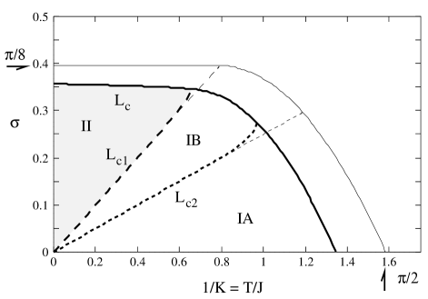
FIG. 3.: Phase diagram for $\gamma=1.6$ (thick lines) and $\gamma=10$ (thin lines). The transition $L_{\rm c}$ (continuous lines) separates the low-temperature phase with quasi long-range order from the disordered high temperature phase. The crossover line $L_{\rm c1}$ (long dashed lines) separates the glassy region II from the non-glassy region I. On the crossover line $L_{\rm c2}$ (short dashed lines) separates regimes IA and IB within phase I. There the disconnected vortex density correlation function changes its asymptotic behavior.

REFERENCES

- [1] M. Rubinstein, B. Shraiman and D.R. Nelson, Phys. Rev. B 27, 1800 (1983).
- [2] E. Granato and J.M. Kosterlitz, Phys. Rev. B 33, 6533 (1986); Phys. Rev. Lett. 62, 823 (1989).
- [3] D.R. Nelson, Phys. Rev. B 27, 2902 (1983).
- [4] J.M. Kosterlitz and D.J. Thouless, J. Phys. C 6, 1181 (1973).
- [5] J.M. Kosterlitz, J. Phys. C 7, 1046 (1974).
- [6] J.L. Cardy and S. Ostlund, Phys. Rev. B 25, 68991 (1982).
- [7] S.E. Korshunov, Phys. Rev. B 48, 1124 (1993).
- [8] Y. Ozeki and H. Nishimori, J. Phys. A 26, 3399 (1993).
- [9] M.G. Forrester, H. Jong-Lee, M. Tinkham and C.J. Lobb, Phys. Rev. B 37 5966(1988); S.P. Benz, M.G. Forrester, M. Tinkham and C.J. Lobb, Phys. Rev. B 38, 2869 (1988).
- [10] A. Chakrabarti and C. Dasgupta, Phys. Rev. B37, 7557 (1988); M.G. Forrester, S.P. Benz, and C.J. Lobb, Phys. Rev. B41, 8749 (1990).
- [11] T. Nattermann, S. Scheidl, S.E. Korshunov, and M.S. Li, J. Phys. I France 5, 565 (1995).
- [12] M.-C. Cha and H.A. Fertig, Phys. Rev. Lett. 74, 4867 (1995).
- [13] S.E. Korshunov and T. Nattermann, preprint (1995).
- [14] G. Parisi, J. Phys. A 13, L115 (1980); J. Phys. A 13, 1101 (1980); J. Phys. A 13, 1887 (1980); Phys. Rev. Lett 50, 1946 (1983); J.-P. Bouchaud and A. Georges, Phys. Rev. Lett. 68, 3908 (1992); J.-P. Naef and A. Canning, J. Phys. I France 2, 247 (1992); H. Steffan and R. Kühn, Z. Phys. B 95, 249 (1994).
- [15] J. Villain, J. Physique (France) 36, 581 (1975).
- [16] J.V. José, L.P. Kadanoff, S. Kirkpatrick and D. Nelson, Phys. Rev. B 16, 1217 (1977).
- [17] A.P. Young, J. Phys. C 11, L453 (1978).
- [18] For screening in ordinary Coulomb gases see D.R. Nelson, in Fundamental Problems in Statistical Mechanics V, ed. E.G.D. Cohen (North-Holland, Amsterdam, 1979); P. Minnhagen and G.G. Warren, Phys. Rev. B. 24, 2526 (1981); J.M. Thijssen and H.J.F. Knops, Phys. Rev. B 38, 9080 (1988).
- [19] S.F. Edwards and P.W. Anderson, J. Phys. F 5, 965 (1975).
- [20] see, e.g, G. Parisi, Phys. Rev. Lett 43, 1754 (1979); or the random energy model as the simplest case of glassy system: B. Derrida, Phys. Rev. lett 45, 79 (1980); B. Derrida, Phys. Rev. B 24, 2613 (1981); D.J. Gross and M. Mézard, Nucl. Phys. B240, 431 (1984).
- [21] L.H. Tang, in preparation.
- [22] S. Scheidl, in preparation.
- [23] D.A. Huse and S. Seung, Phys. Rev. B 42, 1059 (1990); M.A. Moore and S. Murphy, Phys. Rev. B 42, 2587 (1990); M.P.A. Fisher, T.A. Tokuyasu, and A.P. Young, Phys. Rev. Lett. 66, 2931 (1991); M. Cieplak, J.R. Banavar and A. Khurana, J. Phys. A 24, L145 (1991); M.J.P. Gingras, Phys. Rev. B 45, 7547 (1992).
- [24] G. Hackenbroich and S. Scheidl, Physica C 181, 163 (1991).