Shear Flows and Segregation in the Reaction $A+B\rightarrow\emptyset$

Abstract

We study theoretically and numerically the effects of the linear velocity field ${\bf v}=v_{0}y{\bf\hat{x}}$ on the irreversible reaction $A+B\rightarrow\emptyset$. Assuming homogeneous initial conditions for the two species, with equal initial densities, we demonstrate the presence of a crossover time $t_{c}\sim v_{0}^{-1}$. For $t\ll v_{0}^{-1}$, the kinetics are unaffected by the shear and we retain both the effect of species segregation (for $d<4$) and the density decay rate $At^{-\alpha}$, where $\alpha=\min({d\over 4},1)$. We calculate the amplitude $A$ to leading order in a small density expansion for $2\leq d<4$, and give bounds in $d=4$. However, for $t\gg v_{0}^{-1}$, the critical dimension for anomalous kinetics is reduced to $d_{c}=2$, with the density decay rate $Bt^{-1}$ holding for $d\geq 2$. Bounds are calculated for the amplitude $B$ in $d=2$, which depend on the velocity gradient $v_{0}$ and the (equal) diffusion constants $D$. We also briefly consider the case of a non-linear shear flow, where we give a more general form for the crossover time $t_{c}$. Finally, we perform numerical simulations for a linear shear flow in $d=2$ with results in agreement with theoretical predictions.

PACS Numbers: 02.50. -r, 05.40. +j, 47.70. -n, 82.20. -w.

1 Introduction

Recently there has been considerable activity in the field of diffusion limited chemical reactions (see [1–9] and references therein). Many studies have concentrated on the effects of density fluctuations, especially in the one and two species reactions $A+A\rightarrow\emptyset$ and $A+B\rightarrow\emptyset$. In the time dependent case it is well known that for sufficiently low spatial dimensions these fluctuations alter the kinetics. For example, in the two species reaction with equal initial concentrations, the densities decay asymptotically as $t^{-{d\over 4}}$ for $d<4$ [1, 2, 7] - a slower rate than the mean field $t^{-1}$ result. This is closely related to the phenomenon of segregation, where the species separate into A and B rich zones at large times (for $d<4$). These effects are essentially due to inadequate diffusive mixing of the reactants in low dimensions. This allows the initial density fluctuations to persist, leading to the formation of segregated zones.

However, exposure of the system to a shear flow will lead to a modification of these kinetics, as the velocity gradient will allow the chemicals to mix more efficiently. Hence, we might expect that the critical dimension for the onset of anomalous kinetics (and the appearance of segregated zones) might be lowered. In this paper we attempt to confirm these intuitive expectations by focusing on a two species reaction in a linear (Couette) shear flow, in the case where both species have the same diffusion constant $D$, and the same initial density $n_{0}$. Previous work on similar problems includes the study of shear forces on a binary fluid mixture at criticality (see [10] and references therein). More recently studies have been made of reaction-diffusion systems where particles with a same species exclusion rule were subject to a drift [11, 12, 13]. This exclusion rule meant that particles of the same species were forbidden from occupying the same lattice site. New exponents for the asymptotic density decays were reported, with a theoretical justification based on the Burgers equation. Note that our model differs from these cases, both by the nature of the velocity flow (shear not drift), and by the absence of any exclusion rules.

Although very little work has been done on fluctuations in reaction-diffusion-shear systems, a considerable amount is known about diffusion in shear flows [14, 15, 16, 17]. Exact solutions have been given for the positional probability distribution of a Brownian particle released in a linear velocity field. These results will be employed in the analysis of the following sections. We also mention a paper by Yee [18], where a method was given to obtain an approximate analytic solution to a general reaction-convection-diffusion equation. However, this technique is simply a perturbative method for solving the mean field equations, and as such it takes no account of the microscopic density fluctuations. So instead we employ a different method based on a mapping of the microscopic dynamics onto a quantum field theory [6, 7, 8, 19, 20]. This allows for a systematic treatment of the density fluctuations using diagrammatic perturbation theory. In this way we are able to go beyond the traditional rate equations approach, by using the calculational framework of either an effective or a full quantum field theory.

In brief we find, for a linear shear flow with velocity gradient $v_{0}$, a crossover time of order $v_{0}^{-1}$ - at times $t\ll v_{0}^{-1}$ the behaviour of the system is essentially unaffected by the shear. However for $t\gg v_{0}^{-1}$, the critical dimension for the system is reduced from $d_{c}=4$ to $d_{c}=2$, and hence the mean field decay exponent holds in all physically realisable dimensions. In addition, we note in passing that the problem of the single species reaction $A+A\rightarrow\emptyset$ in a shear flow is unlikely to be interesting, as its critical dimension even without shear is already $d_{c}=2$ [1, 2, 6].

Finally, we give an outline of the layout of this paper. In section 2 we give simple arguments for the critical dimension and crossover times for these systems. The mapping to a quantum field theory is carried out in section 3, and in section 4 we perform density calculations in the different regimes, using the field theory formalism. Numerical simulation results are given in section 5, and we present our conclusions in section 6.

2 Decay Rates and Crossover Times

We shall first consider some simple arguments which determine the density decay rates and crossover times induced by the presence of a shear flow. If we neglect the role played by fluctuations, then the mean field result for the densities gives an asymptotic $t^{-1}$ decay. However by using a variant of an argument first put forward by Toussaint and Wilczek [1], we can understand how the density fluctuations alter this result. At $t=0$, these fluctuations ensure that

$$|N_{a}-N_{b}|_{t=0}\sim({n_{0}L^{d}})^{1\over 2},$$ (1)

where $N_{a}$,$N_{b}$ are the number of A,B particles within a volume $L^{d}$. Consequently the initial density difference satisfies:

$$|a-b|_{t=0}\sim\left({n_{o}\over L^{d}}\right)^{1\over 2}.$$ (2)

In the absence of a shear flow, after a time $t$, typically only the initial density excess will remain in a volume of size $(Dt)^{d\over 2}$, as all the other particles in that region will have mutually annihilated. Hence the number of particles remaining in volume $(Dt)^{d/2}$ at time $t$ is $(n_{0}(Dt)^{d\over 2})^{1\over 2}$ (using equation (1)) and we thus obtain a $t^{-{d\over 4}}$ density decay [1, 2, 7]. However, in our case, the presence of the shear flow means that length scales parallel to the velocity flow (in the $x$ direction) increase at a different rate to length scales in perpendicular directions. If we now specialise to the case of linear shear, then it is known (from exact solutions for random walkers in linear velocity flows [14, 15, 16]) that this characteristic length scale grows as $(Dt[1+{1\over 3}(v_{0}t)^{2}])^{1\over 2}$. Consequently, after a time $t$, only the initial density excess will remain in a volume of size $(Dt)^{d-1\over 2}(Dt)^{1\over 2}[1+{1\over 3}(v_{0}t)^{2}]^{1\over 2}$. As a result we expect the densities to decay asymptotically as

$$a\sim b\sim t^{-{d\over 4}}\left[1+{(v_{0}t)^{2}\over 3}\right]^{-{1\over 4}}.$$ (3)

Thus for $t\ll v_{0}^{-1}$, we retain the $t^{-{d\over 4}}$ decay (for $d\leq 4$), with the mean field $t^{-1}$ exponent applying for $d>4$. However for times very much larger than the crossover time $t_{c}\sim v_{0}^{-1}$, we have a different regime:

$$a\sim b\sim\cases{t^{-{(d+2)\over 4}}v_{0}^{-{1\over 2}}&for $d<2$\cr t^{-1}&for $d>2$.\cr}$$ (4)

Note that $d=2$ is the lowest possible dimension for the geometry of our system, so in practice the mean field decay exponent is always retained.

We now briefly consider the case of non-linear shear - a considerably more complicated situation. However, we can give some simple arguments which reveal the crossover time where we expect the shear to begin to alter the dynamics. Consider, for example, the non-linear flow ${\bf v}=v_{0}|y|^{n}$sgn$(y){\bf\hat{x}}$ studied in [17]. The shear flow will disrupt a segregated zone around $y=y_{0}$ when the typical zone length scale $(Dt_{c})^{1\over 2}$ is comparable to the distance over which the top and bottom of the segregated zone are sheared apart. The time $t_{c}$ at which this happens is given by

$$v_{0}t_{c}[(Dt_{c})^{1\over 2}+y_{0}]^{n}-v_{0}t_{c}y_{0}^{n}\sim(Dt_{c})^{1\over 2}.$$ (5)

We can rewrite this relation for $t_{c}$ as

$$v_{0}t_{c}y_{0}^{n}\left[1+{(Dt_{c})^{1\over 2}\over y_{0}}\right]^{n}-v_{0}t_{c}y_{0}^{n}\sim(Dt_{c})^{1\over 2}.$$ (6)

For the case of a linear shear flow ($n=1$), we have recovered our earlier result of a crossover time $t_{c}\sim v_{0}^{-1}$. However for $n\not=1$ and $(Dt_{c})^{1\over 2}\ll y_{0}$, we can expand the bracket in the above equation. This leads to a crossover time

$$t_{c}\sim{1\over v_{0}ny_{0}^{n-1}}=\left[{d\over dy_{0}}(y_{0}^{n}v_{0})\right]^{-1},$$ (7)

valid when

$${D^{1\over 2}\over y_{0}}\left({1\over v_{0}ny_{0}^{n-1}}\right)^{1\over 2}=\left({D\over v_{0}ny_{0}^{n+1}}\right)^{1\over 2}\ll 1.$$ (8)

3 The Field Theory Approach

In order to perform more quantitative calculations for the densities, we need a systematic way of including the effect of microscopic density fluctuations. One way in which this can be achieved is by mapping the microscopic dynamics onto a quantum field theory. The first step in this process is to write down a master equation for the microscopic dynamics. This can then be recast in a second quantised formalism, which may in turn be mapped onto a path integral. All of these steps have been described in detail elsewhere [6, 7, 8, 19, 20], so we simply give the resulting field theoretic action. Defining the fields $\phi$ and $\psi$ in terms of the continuous c-number fields $a$ and $b$, where $\phi={1\over 2}(a+b)$ and $\psi={1\over 2}(a-b)$, we have:

$$S=\int dxdyd^{d-2}zdt\left[2\bar{\psi}(\partial_{t}+v(y)\partial_{x}-D\nabla^{2})\psi+2\bar{\phi}(\partial_{t}+v(y)\partial_{x}-D\nabla^{2})\phi\right.$$

$$\qquad\qquad\qquad\qquad\quad\left.+2\lambda\bar{\phi}(\phi^{2}-\psi^{2})+\lambda(\bar{\phi}^{2}-\bar{\psi}^{2})(\phi^{2}-\psi^{2})-2n_{0}\bar{\phi}\delta(t)\right]$$ (9)

where $\bar{\psi}$ and $\bar{\phi}$ are the response fields. The vertices for this field theory are shown in figure 1, where the propagators for the $\phi$ field are solid lines, and the $\psi$ propagators are dotted lines. Notice that if we neglect the quartic terms in the action, and integrate out the response fields, then we recover the classical (mean field) equations:

$${\partial\psi\over\partial t}+v(y){\partial\psi\over\partial x}=D\nabla^{2}\psi$$ (10)

$${\partial\phi\over\partial t}+v(y){\partial\phi\over\partial x}=D\nabla^{2}\phi-\lambda(\phi^{2}-\psi^{2})+n_{0}\delta(t).$$ (11)

To derive the form of the Green functions we again specialise to a linear velocity field, i.e. $v(y)=v_{0}y$. The equation for the Green functions $G=G_{\psi\bar{\psi}}=G_{\phi\bar{\phi}}$ is:

$$2\left({\partial\over\partial t}+v_{0}y{\partial\over\partial x}-D\nabla^{2}\right)G=\delta(x-x^{\prime})\delta(y-y^{\prime})\delta({\bf z}-{\bf z^{\prime}})\delta(t-t^{\prime}).$$ (12)

This equation has been solved elsewhere [14, 15, 16, 17], in the context of the position probability distribution for a random walker released from the origin in a linear shear flow:

$$G=(4\pi D(t-t^{\prime}))^{-{d\over 2}}\left({3\over(v_{0}(t-t^{\prime}))^{2}+12}\right)^{1\over 2}\times$$ (13)

$$\qquad\quad\exp\left(-{3(x-x^{\prime}-{1\over 2}v_{0}(y+y^{\prime})(t-t^{\prime}))^{2}\over D(t-t^{\prime})[(v_{0}(t-t^{\prime}))^{2}+12]}-{(y-y^{\prime})^{2}\over 4D(t-t^{\prime})}-{({\bf z}-{\bf z^{\prime}})^{2}\over 4D(t-t^{\prime})}\right).$$

Note that for $v_{0}(t-t^{\prime})\ll 1$ the Green function is the essentially same as for a shearless system (with $v_{0}=0$). Physically this result corresponds to the dominance of diffusion over shear on short enough time scales.

Finally, we can use the field theory to define two classical (tree level) quantities. The first of these is the classical density $\langle\phi\rangle_{cl}$, which is the sum of tree diagrams contributing to $\langle\phi\rangle$ (see figure 2, where $\langle\phi\rangle_{cl}$ is represented by a wavy solid line). This sum can easily be evaluated [6, 7], giving

$$\langle\phi\rangle_{cl}={n_{0}\over 1+n_{0}\lambda t},$$ (14)

the same result as would be found by solving the mean field rate equations. The second classical quantity is the response function, which is defined to be the sum of all possible tree diagrams connected to a single propagator. The nature of the vertices ensures that the $\psi$ response function is just the $\psi$ propagator, whereas the $\phi$ response function is given by the diagrammatic sum shown in figure 3 (where it is represented by a thick solid line).

4 Field Theory Density Calculations

Using the formalism presented in section 3, we are now in a position to calculate the densities in the two distinct time regimes. We consider first the case of $2<d\leq 4$ and $v_{0}t\ll 1$, where an effective field theory can be developed. However such a theory turns out to be almost identical to that previously used by Lee and Cardy to study the same two species reaction, but without shear (see [7] for details). The only fundamental difference lies in the slightly modified form of the Green functions (13). However, they are still sufficiently similar to those of Lee and Cardy that our results, to leading order in a small density expansion, reproduce those of [7], and are independent of $v_{0}$. Hence, quoting from [7], we have, for $2<d<4$ and $(n_{0}\lambda)^{-1}\ll t\ll v_{0}^{-1}$:

$$\langle a\rangle,\langle b\rangle\sim{\Delta^{1\over 2}\over(2\pi)^{1\over 2}(8\pi)^{d\over 4}}(Dt)^{-{d\over 4}},$$ (15)

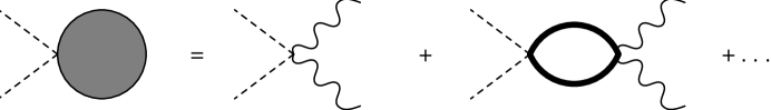
Figure 4: The initial term $\Delta$ is generated by the sum of diagrams shown here. Only the leading order diagram is evaluated.

where $\Delta$ is found by summing the diagrams shown in figure 4, giving $\Delta=2n_{0}$ to leading order in a small density expansion. Note that we require $t\gg(n_{0}\lambda)^{-1}$ so that the coarse-graining required for the calculation of the initial term $\Delta$ is valid. Strictly for this and subsequent results, we must also have $Dt\gg n_{0}^{-2/d}$ - i.e. the particles must have had time to “find” each other by diffusion. For $d=4$ we have the upper bound

$$\langle a\rangle_{upper},\langle b\rangle_{upper}=\left({1\over 2\lambda_{eff}}+\sqrt{{1\over(2\lambda_{eff})^{2}}+{\Delta\over 4(8\pi D)^{2}}}\right)t^{-1},$$ (16)

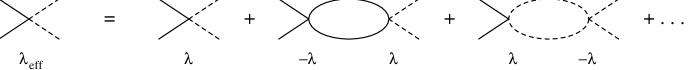
Figure 5: Diagrammatic expansion for the effective coupling constant.

where $\lambda_{eff}$ is an effective coupling constant found by summing the diagrams in figure 5, giving for $v_{0}t\ll 1$:

$$\lambda_{eff}=\lambda\left(1+{2\Lambda^{d-2}\lambda\over(8\pi)^{d/2}(d-2)D}\right)^{-1}.$$ (17)

Here $\Lambda$ is a cutoff which is needed to keep the loop integrals finite. The lower bound for the densities in $d=4$ is given by

$$\langle a\rangle_{lower},\langle b\rangle_{lower}={\Delta^{1\over 2}\over 8\sqrt{2}\pi^{3\over 2}}(Dt)^{-1}.$$ (18)

Finally, it is important to note that these calculations are valid only in the regime $(n_{0}\lambda)^{-1}\ll t\ll v_{0}^{-1}$ and $Dt\gg n_{0}^{-2/d}$. Hence, for small enough $n_{0}$ and large enough $v_{0}$, these conditions will not be satisfied and the above results will not be applicable.

4.1 $v_{0}t\ll 1$ and $d=2$

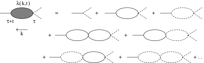
Figure 6: The sum of diagrams contributing to the primitively divergent vertex function $\bar{\lambda}(k,t)$.

Power counting on the full field theoretic action (9) gives $d=2$ as a critical dimension for the system (when $v_{0}t\ll 1$). In this case (of the lowest physically possible dimension), we must consider the full theory, as given by the action (9). The renormalisation is similar to that previously developed in [6, 7, 8], where more details may be found. In particular the field theory remains simple in that diagrams cannot be drawn which dress the propagators. Consequently the bare propagators are the full propagators and both $v_{0}$ and $D$ are not renormalised. Furthermore the simpler form of $G$ for $v_{0}t\ll 1$ again ensures that the results for the $\langle\phi^{2}\rangle$ and $\langle\psi^{2}\rangle$ loops are unchanged from the shearless case [7]. Thus the primitively divergent vertex function $\bar{\lambda}(k,t)$ (figure 6), and resulting $\beta$ function, remain unaltered. Note that we have now rescaled the couplings to absorb the diffusion constant $D$: $\bar{\lambda}=\lambda/D$.

The Callan-Symanzik equation for the densities is slightly modified to read

$$\left[2\bar{t}{\partial\over\partial\bar{t}}-2\bar{v}_{0}{\partial\over\partial\bar{v}_{0}}-dn_{0}{\partial\over\partial n_{0}}-d\Delta{\partial\over\partial\Delta}+\beta(g_{R}){\partial\over\partial g_{R}}+d\right]n(\bar{t},g_{R},n_{0},\bar{v}_{0},\Delta)=0,$$ (19)

where $\bar{v}_{0}=v_{0}/D$, $\bar{t}=Dt$, and $g_{R}$ is the dimensionless renormalised coupling. The solution can be found by the method of characteristics

$$n(\bar{t},g_{R},n_{0},\bar{v}_{0},\Delta)=(\kappa^{2}\bar{t})^{-{d\over 2}}n(\kappa^{-2},\tilde{g}_{R},\tilde{n}_{0},\tilde{\bar{v}_{0}},\tilde{\Delta}),$$ (20)

where $\tilde{n}_{0}=n_{0}(\kappa^{2}\bar{t})^{d\over 2}$, $\tilde{\Delta}=\Delta(\kappa^{2}\bar{t})^{d\over 2}$, and $\tilde{\bar{v}_{0}}=\bar{v}_{0}(\kappa^{2}\bar{t})$. Furthermore, at large enough times (but still such that $v_{0}t\ll 1$), the running coupling $\tilde{g}_{R}$ goes to zero as $(\ln\bar{t})^{-1}$ for $d=2$ [6]. The leading order result is given by (15), and following [7], we make the assumptions that higher order terms are both independent of $n_{0}$, $\bar{v}_{0}$ (and thus of $\tilde{n}_{0}$, $\tilde{\bar{v}_{0}}$), and that they diverge no more quickly than $\tilde{\Delta}^{1\over 2}$, for large $\tilde{\Delta}$. Consequently, if these assumptions are valid, then the densities in $d=2$ will be given by expression (15), with corrections which are suppressed by at least a factor of $(\ln\bar{t})^{-1}$.

4.2 $v_{0}t\gg 1$

At truly asymptotic times $t\gg v_{0}^{-1}$, we can use the Green functions $G=G_{\psi\bar{\psi}}=G_{\phi\bar{\phi}}$ (13) to motivate a new assignment of dimensions for the parameters appearing in the action (9). Firstly we can see from (13) that $[x]\sim[Dv_{0}^{2}t^{3}]^{1\over 2}$. If we ignore the $\partial^{2}_{x}$ terms in the action (corresponding to the neglect of diffusive motion in the $x$ direction) and assign $[\bar{v}_{0}]\sim k^{0}$, then we can give the following naive dimensions:

$$[x]\sim k^{-3}\quad[y],[z]\sim k^{-1}\quad[\bar{t}]\sim k^{-2}\quad[\bar{\lambda}]\sim k^{-d}\quad[\bar{\phi}],[\bar{\psi}]\sim k^{0}\quad[\phi],[\psi]\sim k^{d+2}.$$ (21)

This suggests that a full field theory analysis using the action (9), with subsequent renormalisation, becomes necessary only at dimension $d=0$.

Consequently, following [7], we must now construct a new effective field theory, valid for $d>0$. The first step in this process is to determine which initial parameters are relevant. For an initial term of the type $(\Delta^{(m,n)}/m!n!)\bar{\phi}^{m}\bar{\psi}^{n}|_{t=0}$, we must therefore consider the dimensions of the coupling $[\bar{\lambda}^{m+n}\Delta^{(m,n)}]\sim k^{-d(m+n)+d+2}$. The power of $\bar{\lambda}$ follows from considering the number of vertices needed to attach the initial term to a given diagram. These terms will be relevant when $d<2/(m+n-1)$. Hence, if we have $m+n=1$, then such an initial term is relevant for all $d$. The case of $m=1$ corresponds to the initial density, whereas the generation of an $n=1$ term is forbidden by the invariance of the system under a transformation exchanging $A\leftrightarrow B$, i.e. $(\phi,\bar{\phi},\psi,\bar{\psi})\rightarrow(\phi,\bar{\phi},-\psi,-\bar{\psi})$. The only other important initial terms are those with $m+n=2$, which are marginal in $d=2$. In fact we need only consider an extra initial term of the type $(\Delta^{(0,2)}/2)\bar{\psi}^{2}$, as $\Delta^{(1,1)}$ is forbidden by symmetry, and $\Delta^{(2,0)}$ is suppressed (it can only act as a source of noise through a $\phi$ response function, which we assume to be heavily damped, as in [7]). So, for $d\leq 2$, we are led to the construction of an effective field theory with an extra initial term, whereas for $d>2$ all initial terms (except the initial density) are irrelevant and hence the rate equation approach can be employed. In what follows we shall develop the effective field theory only in $d=2$, as the system cannot be realised in a lower dimension.

Turning to the calculation of $\Delta^{(0,2)}=\Delta$, we again need to sum the set of diagrams shown in figure 4, which for $t\gg(n_{0}\lambda)^{-1}$ gives $\Delta=2n_{0}$ to lowest order in a small density expansion [7]. Aside from this term our action is now linear in the response fields, which we integrate out to yield the equations of motion:

$${\partial\phi\over\partial t}+v_{0}y{\partial\phi\over\partial x}=D\nabla^{2}\phi-\tilde{\lambda}_{eff}(\phi^{2}-\psi^{2})$$ (22)

$${\partial\psi\over\partial t}+v_{0}y{\partial\psi\over\partial x}=D\nabla^{2}\psi,$$ (23)

where $\tilde{\lambda}_{eff}$ is a new effective reaction rate constant, found by summing the diagrams shown in figure 5, giving

$$\tilde{\lambda}_{eff}=\lambda\left(1+{4\sqrt{3}\Lambda^{d}\lambda\over(8\pi)^{d/2}d\bar{v}_{0}D}\right)^{-1},$$ (24)

in the limit $v_{0}t\gg 1$. Note that this result ensures that the density amplitudes are $v_{0}$ dependent even above the upper critical dimension $d_{c}=2$. If we now average equation (22) over the initial conditions, then we have

$${d\over dt}\langle\phi\rangle=-\tilde{\lambda}_{eff}\langle\phi^{2}\rangle+\tilde{\lambda}_{eff}\langle\psi^{2}\rangle,$$ (25)

since $\nabla^{2}\langle\phi\rangle=0$ and $\partial_{x}\langle\phi\rangle=0$. However we can see from a diagrammatic expansion for $\langle\phi\rangle$ (figure 7) that the only diagram contributing to the value of $\langle\psi^{2}\rangle$ in (25) is the single $\psi$ loop, which we now evaluate:

$$\langle\psi^{2}\rangle=\Delta\int dxdyd^{d-2}z\,G(x,y,{\bf z},t)^{2}\qquad\qquad\qquad\qquad\qquad\qquad\qquad\qquad\qquad\$$ (26)

$$\qquad=\Delta\int{dxdyd^{d-2}z\over(4\pi Dt)^{d}}\left({3\over(v_{0}t)^{2}+12}\right)\exp\left\{-{6(x-{1\over 2}v_{0}yt)^{2}\over Dt[(v_{0}t)^{2}+12]}-{y^{2}\over 2Dt}-{{\bf z}^{2}\over 2Dt}\right\}.$$

For $v_{0}t\gg 1$ and $d=2$, this gives the result:

$$\langle\psi^{2}\rangle={\sqrt{3}\Delta\over 16\pi Dv_{0}t^{2}}.$$ (27)

We can now find an upper bound solution to (25) by replacing $\langle\phi^{2}\rangle$ by $\langle\phi\rangle^{2}$ (see [7] for a proof). Calling this upper bound solution $f$, we have for $v_{0}t\gg 1$

$${df\over dt}=-\tilde{\lambda}_{eff}f^{2}+{\tilde{\lambda}_{eff}\Delta\sqrt{3}\over 16\pi Dv_{0}t^{2}}.$$ (28)

This can be solved by making the substitution $f=\dot{u}/\lambda u$, giving the upper bound

$$\langle\phi\rangle\leq f=\left[{1\over 2\tilde{\lambda}_{eff}}+\sqrt{{1\over(2\tilde{\lambda}_{eff})^{2}}+{\Delta\sqrt{3}\over 16\pi Dv_{0}}}\right]t^{-1},$$ (29)

in $d=2$. However, we can also find a lower bound for $\langle\phi\rangle$ by noting that $\phi({\bf x},t)\geq|\psi({\bf x},t)|$, or equivalently that $a({\bf x},t)$ and $b({\bf x},t)$ are everywhere non-negative. We can prove this rigorously using the effective field theory equations for $a$ and $b$:

$${\partial a\over\partial t}=D\nabla^{2}a-v_{0}y{\partial a\over\partial x}-\tilde{\lambda}_{eff}ab$$ (30)

$${\partial b\over\partial t}=D\nabla^{2}b-v_{0}y{\partial b\over\partial x}-\tilde{\lambda}_{eff}ab.$$ (31)

We now assume that the (smooth) fields $a$ and $b$ are initially everywhere non-negative. Suppose, at a later time, $a=0$ at a point, then $a>0$ locally around the point, implying that it is a local minimum. Hence $\nabla^{2}a>0$ and $\partial_{x}a=0$, meaning that $\partial_{t}a>0$. For a region of $a=0$, then we have $\partial_{t}a=0$ inside the region. On its boundaries we have $\nabla^{2}a>0$ and $\partial_{x}a=0$, giving $\partial_{t}a>0$ at these points. As a result the fields cannot pass through zero and will remain non-negative.

Since we have $\phi\geq|\psi|$, it follows that $\langle\phi\rangle\geq\langle|\psi|\rangle$. In addition, at long enough times, we expect $\psi$ to have a normal distribution - a result of $\psi$ satisfying a (modified) diffusion equation. Consequently (as in [7]), we have

$$P[\psi(t)]\propto\exp\left\{-{\psi(t)^{2}\over 2\langle\psi(t)^{2}\rangle}\right\},$$ (32)

and therefore

$$\langle\phi\rangle\geq\langle|\psi(t)|\rangle=\sqrt{{2\over\pi}\langle\psi(t)^{2}\rangle}=\sqrt{\Delta D\sqrt{3}\over 8\pi^{2}v_{0}}(Dt)^{-1},$$ (33)

for $d=2$. However since $\langle g^{2}\rangle\geq\langle g\rangle^{2}$ for any real $g$, then we also have

$$\langle\phi-|\psi|\rangle^{2}\leq\langle(\phi-|\psi|)^{2}\rangle=\langle\phi^{2}\rangle+\langle\psi^{2}\rangle-2\langle\phi|\psi|\rangle,$$ (34)

and using $\phi\geq|\psi|$ this gives us (in $d=2$):

$$\langle\phi-|\psi|\rangle^{2}\leq\langle\phi^{2}\rangle-\langle\psi^{2}\rangle=-{1\over\tilde{\lambda}_{eff}}\langle\dot{\phi}\rangle\sim O(t^{-2}).$$ (35)

In other words, for $d=2$, the bound on the corrections is of the same order as the density. Consequently we cannot say that the density asymptotically approaches the lower bound (as could be said for $(n_{0}\lambda)^{-1}\ll t\ll v_{0}^{-1}$ and $2<d<4$), only that it lies somewhere between the limits supplied by (29) and (33). In this respect the case of $d=2$ and $t\gg v_{0}^{-1}$, $t\gg(n_{0}\lambda)^{-1}$ is similar to that of $d=4$ and $(n_{0}\lambda)^{-1}\ll t\ll v_{0}^{-1}$. In addition both situations retain the $t^{-1}$ mean field decay rate, but with modified amplitudes, which for $d=2$ and $t\gg v_{0}^{-1}$, $t\gg(n_{0}\lambda)^{-1}$ depend on $v_{0}$.

Note that in the limit $\tilde{\lambda}_{eff}^{2}\Delta/\bar{v}_{0}D^{2}\gg 1$, the upper bound reduces to

$$f\approx\sqrt{{D\Delta\sqrt{3}\over 16\pi v_{0}}}(Dt)^{-1},$$ (36)

i.e. the upper and lower limits differ simply by a numerical factor of $(2/\pi)^{1\over 2}$. On the other hand, if $\tilde{\lambda}_{eff}^{2}\Delta/\bar{v}_{0}D^{2}\ll 1$, then $f\approx(\tilde{\lambda}_{eff}t)^{-1}$. In the limit of strong shear, where any reaction zones are broken up almost immediately, we have recovered a mean field decay from this upper bound.

Finally, we can see that the lower bound (33) is of limited usefulness in the small $\Delta$ or large $v_{0}$ limits, as the bound decreases with either increasing $v_{0}$ or decreasing $\Delta$. However, we can use the fact that $\tilde{\lambda}_{eff}^{2}\Delta/\bar{v}_{0}D^{2}$ is dimensionless in $d=2$ to obtain an improved expression for the densities, by performing a perturbation expansion with this parameter. From (25) it follows that the zeroth order term of this series is a constant, equal to the small $\tilde{\lambda}_{eff}^{2}\Delta/\bar{v}_{0}D^{2}$ limit of the upper bound:

$$\langle a\rangle={1\over\tilde{\lambda}_{eff}t}\left[1+{\sqrt{3}\tilde{\lambda}_{eff}^{2}\Delta\over 16\pi\bar{v}_{0}D^{2}}+O\left(\left[{\tilde{\lambda}_{eff}^{2}\Delta\over\bar{v}_{0}D^{2}}\right]^{2}\right)\right].$$ (37)

5 Numerical Results

In order to confirm some of our theoretical predictions we have performed Monte-Carlo simulations in $d=2$. Initially a square lattice of size $L_{x}\times L_{y}$ was populated with equal numbers of randomly distributed A and B particles. The evolution of this initial configuration was simulated using the rare event dynamics (RED) technique (see also [9]). In this Monte Carlo method, the time increment is determined by the current configuration: if many changes in the configuration are likely, then the time increment is small, whereas if the configuration is very stable, the time increment is large. In RED, a list is made of all possible changes to the configuration (events) together with the expected time after which each event will occur (rates). In the present model, two distinct types of events could occur:

(1) A and B particles at $(x,y)$ could hop to neighbouring sites with rates:

UP:	Rate$=1$
DOWN:	Rate$=1$
LEFT:	Rate$=1+s\left({y-0.5L_{y}\over L_{y}}\right)$
RIGHT:	Rate$=1-s\left({y-0.5L_{y}\over L_{y}}\right)$,

where $v_{0}=2s/L_{y}$. Note that the possible values of the shear gradient $v_{0}$ were restricted to ensure that the hop rates remained everywhere positive (i.e. $s\leq 2$).

(2) Each A particle could react with each B particle on the same lattice site, with a reaction rate $\lambda$. The simulations also allowed multiple occupation of each lattice site, in accordance with our theoretical description of the system.

One step in a RED simulation consists of incrementing the time scale with $\Delta t=1/\sum_{j}(r_{j})$, where $r_{j}$ is the rate for event $j$, and then allowing selection (and execution) of an event. The probability that event $i$ is chosen is equal to $p_{i}=r_{i}/\sum_{j}(r_{j})$.

For an efficient implementation the events are organized in a binary tree, where each branch contains one event and has a weight equal to the rate of that event. The weight of a parent node is equal to the sum of the weights of its children. As the root node contains the sum of all rates, the time increment $\Delta t$ is easily obtained: it is the inverse of the weight of the root node. To select a particular event $i$ with a probability proportional to its rate $r_{i}$, we start in the root node, descend to either its left or its right child with a probability proportional to their weights, and iterate this process until we have reached the bottom of the tree. The selected event is then executed and the weights in the tree of all events whose rates have changed, plus their parents, grandparents, etc. are updated. The use of the binary tree assures that the CPU time required for one step in the RED simulation scales with the logarithm of the size of the tree.

In our simulations we have adopted periodic boundary conditions in the direction of the shear flow (in the $x$ direction), but with hard wall boundary conditions perpendicular to it (at $y=0$ and $y=L_{y}$).

The results of simulations on $800\times 200$ and $900\times 300$ lattices are shown in figures 8 and 9 respectively. Data for the shearless cases ($s=0$) are averaged over $20$ runs, whereas those with shear ($s=1$) are averaged over $40$ runs. At very early times the decay is fairly slow (especially in the $n_{0}=0.04$ case) as it takes time for the particles to “find” each other. However at slightly later times we see a straight line for the densities, which is quite well described by the theoretically predicted $t^{-1/2}$ decay. Notice that the simulations both with and without shear are indistinguishable at these early times, indicating that the shear really does have a negligible impact early on (as was predicted in section 4). However for $s\neq 0$, we see a crossover at times of order $v_{0}^{-1}$ to a new regime, which is fairly well described by a $t^{-1}$ decay.

Notice that at late times the densities in the shearless simulations also tail off, and appear to fall away much more quickly than the predicted $t^{-1/2}$ decay. Similar effects were also seen in the original paper by Toussaint and Wilczek [1], where the $t^{-d/4}$ decay (for $d<4$) was first proposed. We interpret this result as being an exponentially fast density decay caused by finite size effects, which become appreciable when the segregated domain sizes become of the same order as the system size. At large enough times these segregated zones will have grown to a size where only two such regions exist (one A rich and the other B rich). The depletion zones of these segregated areas will typically be of the same order as the system length. Hence, if we have just two zones remaining in a system of size $L\times L$, then the densities would decay according to:

$${d\over dt}(L^{2}a)\sim-JL\sim-(aD/L)L\sim-Da,$$ (38)

where $J$ is the flux of particles flowing into the reaction zone. This implies

$$a\sim\exp{(-\rm{(const.)}Dt/L^{2})}.$$ (39)

In order to test this prediction, we simulated an initially completely segregated system of size $200\times 200$. The $t=0$ density profiles for each of the two species were set up to rise linearly from zero (around $y=L_{y}/2$) to a maximum on opposite boundaries (at $y=0$ and $y=L_{y}$). This configuration mimics the effects of having a diffusion length of the same order as the system size. The results of these simulations (averaged over $5$ runs) are shown in figure 10, where an exponential decay is found, in agreement with the above theory.

A further feature of the simulations concerns the effects of the hard wall boundary conditions. Segregated zones neighbouring the hard wall borders at the top and bottom of the system are likely to be more stable, as for these zones fewer reactions are occurring on their boundaries relative to similar regions in the bulk. Hence, if the system is roughly square, then we might expect the reaction zone at late times (when only two segregated regions remain) to lie roughly along $y=L_{y}/2$. This effect has indeed been seen in our simulations in the case of zero shear.

Finally, in figures 11–13, we show the results of various “snapshots” of an $800\times 200$ system as it evolves in the presence of a shear flow. The effects of the shear in tearing apart the reaction zones are clearly illustrated.

6 Conclusion

In this paper we have studied theoretically and numerically the effects of a linear shear flow on the two species reaction $A+B\rightarrow\emptyset$. For $t\ll v_{0}^{-1}$ we found that the system was essentially unaffected by the velocity flow, and the species again segregated into A and B rich zones for $d<4$. In the regime $(n_{0}\lambda)^{-1}\ll t\ll v_{0}^{-1}$ and with $Dt\gg n_{0}^{-2/d}$, our results for the densities (to leading order in a small density expansion) reproduced those of the shearless case [7]. However at large times $t\gg v_{0}^{-1}$, the critical dimension for the onset of anomalous kinetics is reduced from $d_{c}=4$ to $d_{c}=2$. Consequently, for $d\geq 2$, a mean field $t^{-1}$ decay is adopted, though with a modified $v_{0}$ dependent amplitude. Notice, however, that our calculations are for the case of equal diffusion constants. Although it would be possible to treat the case of $D_{A}\not=D_{B}$, we believe (as was found in [7]) that such a modification would be qualitatively unimportant, provided both diffusion constants remain non-zero.

To go beyond the calculations presented in this paper, one could attempt to generalise our analysis to the case of a non-linear shear flow. Unfortunately, excepting the very simple arguments of section 2, it is not clear how to make analytic progress in this case, as the equation for the Green functions (12) becomes very much harder to solve. However, it should prove possible to incorporate into our model a repulsive force between like particles. This would make our system more similar to those considered in [11, 12, 13], where a same species hard core exclusion rule was imposed. In this way we could use the field theoretic formalism to investigate the effects of exclusion on reaction-diffusion systems with shear or drift.

Acknowledgments. The authors would like to thank John Cardy for useful discussions. MJH acknowledges financial support from the EPSRC, and also from Somerville College, Oxford. GTB acknowledges financial support from the EPSRC under grant GR/J78044, from the DOE under grant DE-FG02-90ER40542, and from the Monell Foundation.

Figure 1: Vertices given by the field theoretic action.

Figure 2: The classical density $\langle\phi\rangle_{cl}$, given by (a) the sum over tree diagrams, or (b) an integral equation.

Figure 3: The diagrammatic sum for the $\phi$ response function.

Figure 7: Diagrammatic expansion for $\langle\phi\rangle$, using the initial terms $n_{0}$ and $\Delta$.

Figure 8: Simulation results on an $800\times 200$ system, with $\lambda=1000$, $n_{0}=0.1$, and $s=1$ (diamonds) or $s=0$ (plus signs). The straight lines have gradients of $-0.5$ and $-1$ respectively.

Figure 9: Simulation results on a $900\times 300$ system, with $\lambda=1000$, $n_{0}=0.04$, and $s=1$ (diamonds) or $s=0$ (plus signs). The straight lines have gradients of $-0.5$ and $-1$ respectively.

Figure 10: Simulation results on a $200\times 200$ system with complete initial segregation and $\lambda=1000$, $s=0$.

Figure 11: Snapshot of an $800\times 200$ system, with $s=1$, $n_{0}=0.1$, $\lambda=1000$ at $t=300$.

Figure 12: Snapshot of the same $800\times 200$ system at $t=900$.

Figure 13: Snapshot of the same $800\times 200$ system at $t=1500$.

References

- [1] D. Toussaint and F. Wilczek, J. Chem. Phys. 78, 2642 (1983).
- [2] K. Kang and S. Redner, Phys. Rev. A 32, 435 (1985).
- [3] L. Gálfi and Z. Rácz, Phys. Rev. A 38, 3151 (1988).
- [4] E. Ben-Naim and S. Redner, J. Phys. A 25, L575 (1992).
- [5] S. Cornell and M. Droz, Phys. Rev. Lett. 70, 3824 (1993).
- [6] B. Lee, J. Phys. A 27, 2633 (1994).
- [7] B. Lee and J. Cardy, J. Stat. Phys. 80, 971 (1995).
- [8] M.J. Howard and J. Cardy, J. Phys. A 28, 3599 (1995).
- [9] G.T. Barkema, M.J. Howard, and J.L. Cardy, submitted to Phys. Rev. E
- [10] K. Kawasaki, in Phase Transitions and Critical Phenomena, ed. C. Domb and M.S. Green (Academic Press, London, 1976), Vol. 5a.
- [11] S.A. Janowsky, Phys. Rev. E 51, 1858 (1995).
- [12] S.A. Janowsky, Phys. Rev. E 52, 2535 (1995).
- [13] I. Ispolatov, P.L. Krapivsky, and S. Redner, Phys. Rev E 52, 2540 (1995).
- [14] G.K. Batchelor, J. Fluid Mech. 95, 369 (1979).
- [15] R.T. Foister and T.G.M. Van De Ven, J. Fluid Mech. 96, 105 (1980).
- [16] R. Mauri and S. Haber, SIAM J. Appl. Math. 46, 49 (1986).
- [17] E. Ben-Naim, S. Redner, and D. ben-Avraham, Phys. Rev. A 45, 7207 (1992).
- [18] E. Yee, Phys. Lett. A 151, 295 (1990).
- [19] M. Doi, J. Phys. A 9, 1465 (1976); J. Phys. A 9, 1479 (1976).
- [20] L. Peliti, J. Physique 46, 1469 (1985).