Coherent Charge Transport in Superconductor – Normal Metal Proximity Structures

Abstract

We develop a detailed analysis of electron transport in normal diffusive conductors in the presence of proximity induced superconducting correlation. We calculated the linear conductance of the system and the profile of the electric field. A rich structure of temperature dependences was found and explained. Our results are consistent with recent experimental findings.

Recent progress in nanolithographic technology revived the interest to both experimental and theoretical investigation of electron transport in various mesoscopic proximity systems consisting of superconducting and normal metallic layers. In such systems the Cooper pair wave function of a superconductor penetrates into a normal metal at a distance which increases with decreasing temperature [1]. At sufficiently low temperatures this distance becomes large and the whole normal metal may acquire superconducting properties. Although this phenomenon has been already understood more than thirty years ago and intensively investigated during past decades, recently novel physical features of metallic proximity systems have been discovered [2, 3, 4, 5] and studied theoretically (see [6, 7, 8, 9, 10, 11, 12, 13, 14, 15] and further references therein).

In this paper we study the influence of the proximity effect on transport properties of a diffusive conductor in the limit of relatively low temperatures and voltages. We will assume that this conductor is brought in a direct contact to a superconducting reservoir which serves as an effective injector of Cooper pairs into a normal metal. It is reasonable to assume that in this case the system conductance can only increase in comparison to its normal state value. As the penetration length of Cooper pairs into a normal metal becomes larger with decreasing temperature $T$ one might expect the system conductance to increase with $1/T$ monotoneously. In what follows we shall present a rigorous calculation of a temperature dependent linear conductance of the the system and demonstrate that its actual temperature dependence turns out to be more complicated. In particular we will show that if the system contains no tunnel barriers there are two different physical regimes which determine the system conductance in different temperature intervals. At relatively high temperatures the superconducting correlation of electrons in the normal metal survives at the typical distance of order $\xi_{N}\sim\sqrt{{\cal D}/T}$, where ${\cal D}=v_{F}l_{imp}/3$ is the diffusion coefficient. As $T$ is lowered proximity induced superconductivity expands into the normal metal and, consequently, the “normally conducting” part of the system effectively shrinks in size. This effect results in increasing of the conductance of a normal metal. At sufficiently low temperature the length $\xi_{n}$ becomes of order of the size of the normal layer, i.e. the superconducting correlation survives everywhere in the normal metal and the effective gap in the quasiparticle spectrum develops there [16]. Physically this means that at sufficiently low energies and temperatures there exist no uncorrelated electrons in the normal metal with a superconducting reservoir attached to it. The characterisic energy which plays the role of such a gap is $\varepsilon_{g}\sim\min(\Delta,D/L^{2})$. At energies lower than this value electron transport is only due to such correlated electrons (or Cooper pairs injected into the N-metall) which “density of states” increases with increasing $\varepsilon$ due to the gap effect. As the temperature is increased from zero higher and higher values of $\varepsilon$ contribute to the current and the system conductance increases with $T$ at very low temperatures. Eventually with increasing $T$ a crossover to a high temperature behavior of the system conductance takes place. Note that similar behavior of the normal metal conductance in the presence of proximity-induced superconductivity has been also found in a recent numerical analysis by Nazarov and Stoof [21]. It is also interesting to point out that at $T=0$ the system conductance coincides with that of a normal metal with no proximity effects [17].

We will also demonstrate that in the presence of tunnel barriers the temperature dependence of the conductance is essentially different. Whereas the contribution of the diffusive region is nonmonotoneus in T, the conductance of the interfaces decreases monotonously with temperature. At the same time the proximity-induced superconducting gap developes in N [16]. As a result, with lowering the barrier transparency the crossover takes place to the effective conductance decreasing monotonously with T, characteristic for two serial NIS’ tunnel junctions (S’ is now the diffusive normal conductor with proximity-induced gap). We note that both types of behavior, namely nonmonotonously enhanced and monotonously decreasing with T conductance have been observed in the experiment [3].

Let us consider a a quasi-one-dimensional normal conductor of a length $2L$ with a superconducting strip of a thickness $2d_{s}$ attached to a normal metal on the top of it and two normal reservoirs attached to its edges (see fig.1). The length $L$ is assumed to be much larger than the elastic mean free path $l_{imp}$ but much shorter than the inelastic one. This geometrical realization has a direct relation to that investigated in the experiments [3, 5]. The two big normal reservoirs N’ are assumed to be in thermodynamic equilibrium at the potentials $V$ and $0$ respectively. In contrast to the case of ballistic constriction [18] the potential drop within the system is distributed between the interfaces and the conductor itself. The general approach to calculate the conductance of such kind of structures was developed in [6, 7, 8]. In what follows we shall apply this method to analyse the temperature dependence of the NS proximity structure of fig.1.

The electron transport through the metallic system can be described by the equations for a matrix of quasiclassical Green functions$\stackrel{{\scriptstyle\vee}}{{G\text{ }}}$in the contact [19, 20]:

$$\stackrel{{\scriptstyle\vee}}{{G\text{ }}}=\left(\begin{array}[]{cc}\stackrel{{\scriptstyle\wedge}}{{G}}^{R}&\stackrel{{\scriptstyle\wedge}}{{G}}^{K}\\ 0&\stackrel{{\scriptstyle\wedge}}{{G}}^{A}\end{array}\right)$$ (1)

where $\stackrel{{\scriptstyle\wedge}}{{G^{A}}}$, $\stackrel{{\scriptstyle\wedge}}{{G^{R}}}$ and $\stackrel{{\scriptstyle\wedge}}{{G^{K}}}$ are respectively the impurity-averaged advanced, retarded and Keldysh Green functions. These functions are in turn matrices in the Nambu space:

$$\stackrel{{\scriptstyle\wedge}}{{G^{R}}}=\stackrel{{\scriptstyle\wedge}}{{\sigma_{z}}}g^{R}+\stackrel{{\scriptstyle\wedge}}{{i\sigma_{y}}}f^{R},\stackrel{{\scriptstyle\wedge}}{{G^{A}}}=-(\stackrel{{\scriptstyle\wedge}}{{G^{R}}})^{*}\hbox{and}\stackrel{{\scriptstyle\wedge}}{{G^{K}}}=\stackrel{{\scriptstyle\wedge}}{{G^{R}}}\stackrel{{\scriptstyle\wedge}}{{f}}-\stackrel{{\scriptstyle\wedge}}{{f}}\stackrel{{\scriptstyle\wedge}}{{G^{A}}}$$

. Here the distribution function $\stackrel{{\scriptstyle\wedge}}{{f}}=f_{l}+\stackrel{{\scriptstyle\wedge}}{{\sigma_{z}}}\stackrel{{\scriptstyle\wedge}}{{f_{t}}}$, where $f_{l}=\tanh(\varepsilon/2T)$ and $\stackrel{{\scriptstyle\wedge}}{{f_{t}}}$ describes deviation from nonequilibrium. Taking advantage of the normalization condition for the normal and the anomalous Green functions $(g^{R})^{2}-|f^{R}|^{2}=1$ it is convenient to parametrize $g^{R}=\cosh\theta,$ $f^{R}=\sinh\theta$, where $\theta\equiv\theta_{1}+i\theta_{2}$ is a complex function. Deep in the bulk superconductor it is equal to $\theta_{s}=1/2\ln\left[(\Delta+\varepsilon)/(\Delta-\varepsilon)\right]-i\pi/2$ for $\varepsilon<\Delta$ and $\theta_{s}=(1/2)\ln\left[(\varepsilon+\Delta)/(\varepsilon-\Delta)\right]/2$ for $\varepsilon>\Delta$ (here and below we omit the indices R(A)).

The electrical current $I$ and the electrostatic potential $\phi$ are expressed through $\stackrel{{\scriptstyle\vee}}{{G\text{ }}}$ as

$$I=\frac{\nu{\cal D}S}{2}\int_{-\infty}^{\infty}d\varepsilon\text{ }Sp\left[\stackrel{{\scriptstyle\wedge}}{{\sigma_{z}}}\stackrel{{\scriptstyle\vee}}{{G\text{ }}}\partial_{x}\stackrel{{\scriptstyle\vee}}{{G\text{ }}}\right]^{K},$$ (2)

$$\phi(x)=\int_{0}^{\infty}d\varepsilon\,\hbox{Tr}\hat{g}^{K}(x,\varepsilon)=\int_{0}^{\infty}d\varepsilon\,f_{t}(x,\varepsilon)\nu_{\varepsilon}(x),$$ (3)

where $\nu$ is the the density of states, $\nu_{\varepsilon}(x)=\Re(g^{R}_{\varepsilon}(x))$ and $S$ is the crossection area of $N$ conductor.

Being expressed in terms of the function $\theta(\varepsilon,x)$ the equations [19, 20] for the Green functions and the distribution function for the N-metall take a particularly simple form

$${\cal D}\partial_{x}^{2}\theta+2i\varepsilon\sinh\theta=0$$ (4)

$$\partial_{x}\left[{\cal D}(\cosh^{2}\theta_{1})\partial_{x}f_{t}\right]=0,$$ (5)

$x$ is the coordinate along the N-conductor. Here we neglected the processes of inelastic relaxation and put the pair potential in the normal metal equal to zero $\Delta_{N}=0$ assuming the absence of electron-electron interaction in this metal.

Before we come to a detailed solution of the problem let us point out that the conclusion about the anomalous behavior of the system conductance can be reached already from the form of eq. (5). Indeed it is quite clear from (5) that the effective diffusion coefficient increases in the N-regions with proximity-induced superconductivity and, therefore, the electric field is partially expelled from these regions. This energy dependent field modulation is controlled by the solution for $\theta(\varepsilon,x)$ and is directly related to the physical origin of the anomalous temperature dependence of the system conductance discussed below.

The equations (4) and (5) should be supplemented by the boundary conditions at the interfaces of the normal metall N. Assuming that the anomalous Green function of big normal reservoirs N’ is equal to zero from [22, 7] we obtain

$$\begin{array}[]{c}\gamma_{B}\partial_{x}\theta=\sinh\theta\\ \gamma_{B}\cosh\theta_{1}\partial_{x}f_{t}=\cosh\theta_{1}(f_{t}-f_{t}(x=0,2L)),\end{array}$$ (6)

where $\gamma_{B}=R_{b}/\rho_{N}$ is the interface resistance parameter, $R_{b}$ is the resistance of the interface between the N-conductor and the N’-reservoirs, $\rho_{N}$ is the resistivity of the N-metal. In general we should also fix the boundary condition at the interface between the N-metal and the superconductor. For the case of a perfect transparency of this interface (which is only considered here) and for typical thickness of the normal layer $w_{N}\sim\sqrt{S}\\ \xi_{N}$ Cooper pairs easily penetrate into it due to the proximity effect and the Green functions of the N-metal at relatively low energies for $d\leq x\leq d+2d_{s}$ are equal to those of a bulk superconductor $\theta=\theta_{s}$. This intuitively obvious result can be proven rigorously (see e.g. [15] and references therein). Thus the region of a normal metal situated directly under the superconductor for our purposes can be also considered as a piece of a superconductor S’ and the solution of (4), (5) needs to be found only for $0<x<d$ (without loss of generality we will stick to a symmetric configuration).

Proceeding along the same lines as it has been done in ref. [8] we arrive at the final expression for the current

$$I=\frac{1}{2R}\int_{0}^{\infty}d\varepsilon\left[\tanh((\varepsilon+eV)/2T)-\tanh((\varepsilon+eV)/2T)\right]D(\varepsilon),$$ (7)

where $D(\varepsilon)$ defines the effective transparency of the system [8]

$$D(\varepsilon)=\frac{L+\gamma_{B}}{\frac{\gamma_{B}}{\cosh\theta_{2}(x=0,\varepsilon)\cos\theta_{1}(x=0,\varepsilon)}+\int_{0}^{L}dx\,\hbox{sech}^{2}\theta_{1}(x,\varepsilon)}.$$

Let us consider the case of a sufficiently long normal conductor $d\gg{\cal D}/\Delta$. Then at low temperatures $T\ll\Delta$ the interesting energy interval is restricted to $\varepsilon\ll\Delta$. For such values of $\varepsilon$ the contribution of the $S^{\prime}$-part of the normal conductor shows no structure and can be easily taken into account with the aid of obvious relations

$$\int_{0}^{L}dx\,\hbox{sech}^{2}\theta_{1}(x,\varepsilon)=\int_{0}^{d}dx\;\hbox{sech}^{2}\theta_{1}(x,\varepsilon)+d_{s}\hbox{sech}^{2}\theta_{s,1}$$ (8)

and $\hbox{sech}^{2}\theta_{s,1}=\left(1-{\varepsilon^{2}\over\Delta^{2}}\right)$. Due to this reason we will discuss only the properties of the $N$-part ($0<x<d$). For the sake of completeness we will also demonstrate the effect of finite $d_{s}$ in the end of our calculation.

For the differential conductance of the $N$-part $0\leq x\leq d$ normalized to its normal (“non-proximity”) value in the zero bias limit eq. (7) yields

$$\bar{\sigma}_{N}=\left({RdI\over dV}\right)_{V=0}={1\over 2T}\int_{0}^{\infty}d\varepsilon{D(\varepsilon)\hbox{sech}^{2}(\varepsilon/2T)}.$$ (9)

Analogously the normalized zero-bias electrostatic potential distribution reads

$$\phi_{0}(x)=\lim_{V\rightarrow 0}{\phi(x)\over V}={1\over 2Td}\int_{0}^{\infty}d\varepsilon\,D(\varepsilon)\nu_{\varepsilon}(x)\hbox{sech}^{2}(\varepsilon/2T)\int_{x}^{d}dx^{\prime}\,\hbox{sech}^{2}(\theta_{1}(x^{\prime}))$$ (10)

The analysis of the problem can be significantly simplified in the case of perfectly transparent interfaces ($\gamma_{B}=0$). In this case the boundary conditions are

$$\theta(0) = 0$$ (11)

$$\theta(d) = \theta_{S}$$ (12)

for the contact to the normal and the superconducting reservoir respectively. The effective transparency of the N-part then reads

$$D(\varepsilon)=\left({1\over d}\int_{0}^{d}dx\;\hbox{sech}^{2}(\theta_{1}(x))\right)^{-1}.$$ (13)

As it was already pointed out for relatively long normal conductors and at low $T$ only the energies $\varepsilon\ll\Delta$ give an important contribution to the conductance. In this case the typical energy scale is defined by the Thouless energy $\epsilon_{d}={\cal{D}/d^{2}}\ll\Delta$. For these energies we can set $\theta_{S}=i{\pi/2}$. Let us first put $T=0$. Then the thermal distribution factor $\beta\,\hbox{sech}^{2}(\beta\varepsilon)$ reduces to a delta function and we have

$$\bar{\sigma}_{N}(T=0)=D(0),$$ (14)

$$\phi_{0}(x)=(D(0)\nu_{0}(x)/d)\int_{x}^{d}dx^{\prime}\hbox{sech}^{2}(\theta_{1}(x^{\prime})),$$ (15)

i.e. we only need the solution of (4) with boundary conditions (11) at $\varepsilon=0$, which is $\theta=i{\pi\over 2}{\bar{x}}$ and therefore $\nu_{0}(x)=\cos(\bar{x}\pi/2)$, where $\bar{x}=x/d$. This means

$$\bar{\sigma}_{N}(T=0)=1.$$ (16)

This result coincides with that obtained first by Artemenko, Volkov and Zaitsev [17] and demonstrates that – in contrast to what one might expect intuitively – at $T=0$ and very low voltages the diffusive conductor does not “feel” the proximity-induced superconductivity and the conductance is exactly equal to its normal state value. The profile of the electric field penetrating into the normal metal at $T=0$ also can be found easily. We have

$$E_{0}(x):={\partial_{\bar{x}}}\phi_{0}(x)={\pi\over 2}(\bar{x}-1)\sin(\bar{x}\pi/2)-\cos(\bar{x}\pi/2),$$ (17)

i.e. in the low temperature limit the electrical field distribution in the structure turns out to be essentially nonmonotoneous. In the case $T\ll\varepsilon_{d}$ we can calculate $\theta$ perturbatively. From $\cal{D}\partial_{x}^{2}\theta=-2i\varepsilon\sinh\theta_{0}(x)$ and (11) we get

$$\theta={8\over\pi^{2}}{\varepsilon\over\varepsilon_{d}}[\bar{x}-\sin(\bar{x}\pi/2)]+i{\pi\over 2}\bar{x}.$$

Keeping only leading order terms in $\epsilon\over\epsilon_{d}$, we get

$$\bar{\sigma}_{N}=1+A{T^{2}\over\epsilon_{d}^{2}},$$ (18)

where $A={128\over\pi^{4}}\left({5\over 6}-{8\over\pi^{2}}\right)\zeta(2)\approx 0.049$ is a universal constant. This means, that for low temperatures $\bar{\sigma}_{N}(T)$ grows quadratically on the scale of $\varepsilon_{d}$ and approaches the crossover towards the high temperature regime discussed below.

We can also calculate the electrical field distribution in this approximation, however, the result is rather cumbersome and shows no structure which could not be seen from the numerical results presented below.

In this limit $T\gg\epsilon_{d}$ (where we still have $T\ll\Delta$), the contribution of the low energy components to the thermally weighted integrals for $\bar{\sigma}_{N}(T)$ and $\phi_{0}(T)$ is neglible and we only have to take into account the solutions of (4) for energies $\epsilon\gg\epsilon_{d}$. It is well known (see e.g. [8]), that for this energy range the solution of (4) together with (11) reads

$$\tanh(\theta(\bar{x})/4)=\tanh\left({i\pi\over 8}\right)e^{k(\bar{x}-1)}$$ (19)

where $k=d\sqrt{-2i\varepsilon/\cal{D}}$. By using obvious substitutions and multiple-argument relations for hyperbolic functions, we arrive at the following identity:

$${\int_{\bar{x}}^{1}}d\bar{x}\,\hbox{sech}(\theta_{1}(\bar{x}))=(1-\bar{x})-4\sqrt{\varepsilon_{d}\over\varepsilon}\int_{0}^{\Re(k)(1-\bar{x})}dy\,q(y)/(1+q(y))^{2}$$ (20)

where $q(y)=4(3+2\sqrt{2}){e^{-2y}\sin^{2}y/\left(e^{-2y}+3+2\sqrt{2}\right)^{2}}$.

For calculating $D(\varepsilon)$ we can, as the integrand becomes exponentially small for $y\geq\Re(k)\gg 1$, take the upper bound to infinity, such that it becomes a universal constant. From there we can calculate the conductivity in this limit

$$\bar{\sigma}_{N}(T)=1+B\sqrt{\varepsilon_{d}\over T},$$ (21)

where again $B=0.42$ is a universal constant. The whole integral in the rhs of (20) is very small compared to one, so near the normal reservoir only the $1-\bar{x}$-term has to be kept. As in this region $\nu$ is, apart from exponentially small terms, constant, $\phi_{0}$ is linear in $\bar{x}$, so there $E_{0}$ is constant.

These results have a simple physical interpretation. Superconductivity penetrates into the normal part up to $\xi_{N}=\sqrt{D\over 2\pi T}$, whereas the rest stays normal, so the total voltage drops over a reduced distance $d-\xi_{N}$. Thus the resistance of the structure is reduced according to the Ohm law. In terms of the conductividy, this means

$$\bar{\sigma}_{N}=1+B^{\prime}{\xi_{N}\over d}$$ (22)

which is equivalent to (21).

For temperatures comparable to $\varepsilon_{d}$ the problem can only be handled numerically. The results show excellent agreement to the analytical calculations in the corresponding limits.

The numerical results (see fig 2) confirm, that for $\varepsilon_{d}\ll\Delta$ the universal scaling with $T\over\varepsilon_{d}$ is excellently fulfilled, as even the peak in the conductivity is systematically at $T\approx 5\varepsilon_{d}$ and the peak height of about 9% seems to be universal. This result also agrees with the recent numerical analysis [21]. This peak becomes smaller if we take into account the effect of finite $d_{S}$ keeping $d$ fixed (fig. 3) The qualitative features, however, remain the same.

For the field distribution at $T\ll\varepsilon_{d}$ we can observe the described nonmonotoneous behavior (see fig. 4). From $T\approx\varepsilon_{d}$ also a minimum in the distribution shows up. For $T\gg\varepsilon_{d}$ the electrical field is almost constant for $\bar{x}<1-\xi_{N}/d$, drops rapidly for $\bar{x}>1-\xi_{N}/d$ and shows some interesting structure around $\bar{x}=1-\xi_{N}/d$.

Perhaps the most interesting effect found here is the nonmonotoneous dependence of the system conductance with temperature accompanied by a nontrivial shape of the electric field penetrating in the N-layer. As $T$ is lowered proximity induced superconductivity in this layer becomes stronger and stronger being more and more efficient in expelling the field from the region adjacent to a superconductor. At very low temperatures this results in a substantial suppression of this field in a big part of the sample. Inevitably (the total potential drop is fixed!) this effect leads to an excess value of the electric field far from the NS boundary as it is shown in fig.4. As it was already pointed out we can understand the effect of increase of the system conductance with increasing $T$ at very low temperatures as a gap effect. At $T\sim\varepsilon_{d}$ the conductance reaches its maximum and starts decreasing due to weakening of the proximity with further increase of $T$.

Finally we would like to point out that the presence of tunnel barriers at NN’ interfaces entirely changes the conductance of the system. If one lowers the barrier transparency the crossover takes place to the behavior demonstrating monotonously decreasing conductance with T (fig.5), which is typical for two serial NIS’ tunnel junctions. Note that both types of behavior, namely nonmonotoneous and monotonously decreasing with T conductance have been observed in the experiment [3]. Further details will be presented elsewhere [23].

We would like to thank G. Schön, C. Bruder and W. Belzig for useful discussions. This work was supported by the Deutsche Forschungsgemeinschaft within the Sonderforschungsbereich 195.

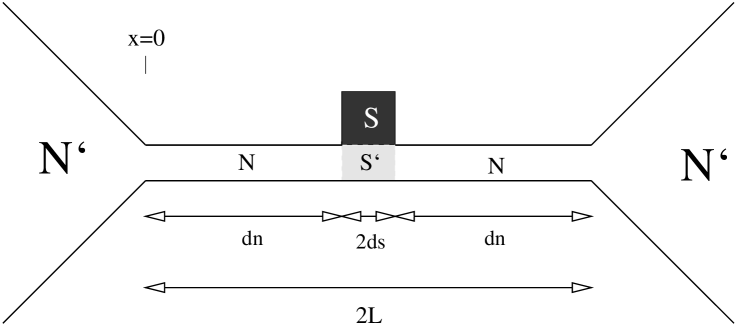
FIG. 1.: Physical setup. $N^{\prime}$ designates normal reservoirs, $S$ superconductor, $S^{\prime}$ is effectly superconducting due to the proximity to $S$, $N$ is the normal part affected by the proximity to $S^{\prime}$

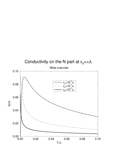
FIG. 2.: Temperature dependence of the conductivity

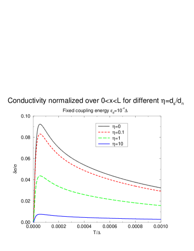
FIG. 3.: Influence of finite $d_{s}$

FIG. 4.: Field distribution for various temperatures

FIG. 5.: Destruction of the structure of $\sigma$ by the presence of strong tunneling barriers

REFERENCES

- [1] P.G. de Gennes. Superconductivity of metals and alloys.
- [2] A.Kastalsky et al., Phys. Rev. Lett. 67, 3026 (1991).
- [3] V.T.Petrashov et al., Phys.Rev. Lett. 74, 5268 (1995).
- [4] H.Pothier et al., Phys. Rev. Lett. 73, 2488 (1994).
- [5] H. Courtois et al., Phys. Rev. B 52, 1162 (1995); Phys. Rev. Lett. 76, 130 (1996).
- [6] A.V.Zaitsev, JETP Lett. 51, 41 (1990).
- [7] A.F.Volkov, JETP.Lett. 55, 747 (1992).
- [8] A.F.Volkov, A.V.Zaitsev, and T.M.Klapwijk, Physica C 210, 21 (1993).
- [9] C.W.J.Beenakker, Phys.Rev.B 46, 12841 (1992).
- [10] C.W.J.Beenakker, B.Rejaei, and J.A.Melsen, Phys.Rev.Lett. B 72, 2470 (1994).
- [11] W.J.Hekking and Yu.V.Nazarov, Phys.Rev.Lett. 71, 1625 (1993).
- [12] Yu.V.Nazarov, Phys.Rev.Lett. 73, 134 (1994).
- [13] A.D.Zaikin, Physica B 203, 255 (1994)
- [14] F.Zhou, B.Spivak and A.Zyuzin, Phys. Rev. B 52, 4467 (1995).
- [15] F.Wilhelm, G.Schön, and A.D.Zaikin, in preparation.
- [16] A.A.Golubov and M.Yu.Kupriyanov, Sov. Phys. JETP 69, 805 (1989); JETP Lett. 61, 855 (1995).
- [17] S.N.Artemenko, A.F.Volkov, and A.V.Zaitsev, Sol. St. Comm. 30, 771 (1979).
- [18] G.E.Blonder, M.Tinkham,and T.M.Klapwijk, Phys.Rev.B 25, 4515 (1982).
- [19] G.M.Eliashberg, Sov.Phys.JETP 34, 668 (1971).
- [20] A.I.Larkin and Yu.N.Ovchinnikov, Sov.Phys.JETP 41, 960 (1975).
- [21] Yu.V.Nazarov and T.H.Stoof. Diffusive Conductors as Andreev Interferometers (preprint).
- [22] M.Yu.Kupriyanov and V.F.Lukichev, Sov.Phys.JETP 67, 1163 (1988).
- [23] A.A.Golubov, F.Wilhelm, and A.D.Zaikin, in preparation.