Material-specific gap function in the high-temperature superconductors

Abstract

We present theoretical arguments and experimental support for the idea that high-$T_{c}$ superconductivity can occur with $s$-wave, $d$-wave, or mixed-wave pairing in the context of a magnetic mechanism. The size and shape of the gap is different for different materials. The theoretical arguments are based on the $t$-$J$ model as derived from the Hubbard model so that it necessarily includes three-site terms. We argue that this should be the basic minimal model for high-$T_{c}$ systems. We analyze this model starting with the dilute limit which can be solved exactly, passing then to the Cooper problem which is numerically tractable, then ending with a mean field approach. It is found that the relative stability of $s$-wave and $d$-wave depends on the size and the shape of the Fermi surface. We identify three striking trends. First, materials with large next-nearest-neighbor hopping (such as YBa₂Cu₃O_7-x) are nearly pure $d$-wave, whereas nearest-neighbor materials (such as La_2-xSr_xCuO₄) tend to be more $s$-wave-like. Second, low hole doping materials tend to be pure $d$-wave, but high hole doping leads to $s$-wave. Finally, the optimum hole doping level increases as the next-nearest-neighbor hopping increases. We examine the experimental evidence and find support for this idea that gap function in the high-temperature superconductors is material-specific.

]

I Introduction

In the years following the discovery of the high-$T_{c}$ materials, theoretical debate often centered on the anomalous normal state properties, these being seen as the key to understanding the underlying physics. The superconducting state, by contrast, was generally thought to be conventional except for its coupling strength. More recently, however, it has seemed more reasonable to regard the superconducting state, especially the gap symmetry, as holding the key to theoretical understanding. Recent experimental progress gives hope that the gap symmetry can be unraveled. Once this is done, one expects that very strong constraints can be placed on the microscopic model. This will certainly be true if, as we shall contend in this paper, different high-$T_{c}$ systems have different gap functions.

The early consensus that the high-$T_{c}$ superconductors are $s$-wave has been replaced by the view that they are most likely $d$-wave. Support for this latter position has come primarily from three experimental sources: penetration depth measurements [3, 4], photoemission measurements [5, 6], and Josephson interference measurements [7, 8, 9]. These results very much strengthened the idea that the mechanism is magnetic. Even before the discovery of high-$T_{c}$ superconductivity it was clear that magnetic interactions based on antiferromagnetic correlations would quite naturally give rise to a tendency toward higher-wave pairing [10, 11], and studies of the $t$-$J$ model [12, 13] and the Hubbard model [14] around the time of the discovery confirmed this for the CuO₂ square lattice . A more complete theory, though one which requires some phenomenological input, has been constructed on the hypothesis that antiferromagnetic spin fluctuations act very much like the phonons in low-$T_{c}$ materials and cause the pairing [15, 16]. This theory, which we shall call the spin-fluctuation model, requires the presence of very strong spin correlations which lead to a high critical temperature and to $d$-wave pairing.

If it is accepted that a magnetic mechanism is responsible for high-$T_{c}$, there still remain many outstanding issues. The spin-fluctuation model generally relies on a pairing interaction which is very well localized in momentum space. The interaction is proportional to the magnetic susceptibility, which is taken to be very strongly peaked near the $k_{x}=\pm\pi/a$ and $k_{y}=\pm\pi/a$ points. The spin-fluctuation model leads unambiguously to $d$-wave superconductivity and not to $s$-wave. This also appears to be the case in the spin bag model, although the range of the interaction is shorter in this case, of order $\hbar v_{F}/\Delta_{\text{SDW}}$, where $v_{F}$ is the Fermi velocity and $\Delta_{\text{SDW}}$ is the charge density wave gap of the ordered phase [17]. On the other hand, theories based on the $t$-$J$ model rely on a spin-spin interaction which is rather local in real space. We shall call this the spin-interaction model. If the gap equation is solved in this model, substantial regions of both $s$-wave and $d$-wave pairing are found [12]. In earlier variational Monte Carlo (VMC) calculations on this model, the dominant instability of the normal state was toward $d$-wave pairing, but in some parameter regimes there was also the possibility of admixture of $s$-wave symmetry into the ground state [18]. Thus, although the spin-interaction model clearly falls into the category of magnetic mechanisms, it is distinct from the spin-fluctuation model in that it predicts that the gap symmetry is not necessarily always pure $d$-wave. Rather, $s$-wave and $d$-wave are competing instabilities. This latter direction of inquiry has been briefly summarized by Müller, who notes that the possible coexistence of $s$- and $d$-wave can describe recent experimental results [19]. Our Sec. VII is an expansion of this theme.

The comparison of the spin-fluctuation model and the spin-interaction model leads to the conclusion that all magnetic mechanisms are not alike. Even if it is conceded that the basic mechanism for high-$T_{c}$ superconductivity is magnetic, there is still work to be done. This paper is written to amplify and sharpen this point.

We present a brief discussion of recent theoretical work which is directly relevant to the issue material-specific gap functions (Sec. II) arising from the magnetism mechanism. The extended $t$-$J$ model is developed from the overlapping copper and oxygen orbitals in the CuO₂ planes (Sec. III). We point out physical reasons to support the idea of $s$- and $d$-wave as competing instabilities based upon the solution of the $t$-$J$ model in the dilute limit (Sec. IV). It is noted that this solution in fact corresponds to a physical limit of the gap equation in which the interactions do not possess a frequency cutoff. We then extend our arguments by solving the Cooper problem with the $t$-$J$ model (Sec. V). We follow with a presentation of a mean field approach to the $t$-$J$ model which does indeed yield mixed $s$- and $d$-wave pairing under certain circumstances (Sec. VI). Finally, we survey existing experiments and find evidence of the trends identified in the analysis of our model (Sec. VII). The approach of the experimental survey is to examine different materials one by one in order to see if they all have the same gap symmetry. Our conclusion is that the details of the gap function are material-specific, and that this lends support for using the $t$-$J$ model, extended in an appropriate fashion, as a basic, yet flexible description of high-temperature superconductivity in the cuprate-layered materials.

II Theoretical Background

Admirably complete and comprehensive surveys of theoretical work on the magnetic mechanism and the question of d-wave pairing has recently been carried out by Scalapino [20] (see particularly Appendix A, and references therein), Dagotto [21], and von der Linden [22], who stress the numerical work. They conclude that numerical evidence from quantum Monte Carlo, variational Monte Carlo, and exact diagonalization on small systems favors d-wave pairing. Certain diagrammatic studies confirm this. These references also point out that the evidence is far from conclusive. For example, quantum Monte Carlo searches for a finite superfluid density in the two-dimensional Hubbard model have not been successful. Thus, studies of d-wave superconductivity in magnetic models are highly suggestive, but we are not assured that superconductivity exists in these microscopically justified models.

Our approach in this paper is to sidestep this thorny issue. Instead of investigating the microscopic models with the most sophisticated tools available to ask whether superconductivity is present, we shall use simple mean-field-type methods which are expected to give superconductivity. The idea is to apply these methods to rather more complicated models, intended to more closely mimic the actual systems. If we can identify trends as a function of the (fairly numerous) parameters in the models, these may then be compared to experiment in a detailed way. Accordingly, we do not review those studies which have been carried out on the nearest-neighbor Hubbard model or its strong-coupling equivalent, the nearest-neighbor $t$-$J$ model, the aim of which has generally been to search for pure d-wave superconductivity. Our interest is in the question of whether the gap structure may be material-specific. Specifically, we wish to address the issue of whether the shape and size of the gap function may depend on details of the band structure and the doping level. We therefore review here those papers which treat more complex models or more complicated gap functions.

The finding of a more complex gap structure in the $t$-$J$ model originates from the very beginning of this field of study. Ruckenstein et al., were among the first to apply this model for use in calculating some of physical parameters of the high-temperature superconductors [12]. They analyzed the model with a mean field treatment (similar to Sec. VI), and found a parameter range where a mixture of $s$-wave and $d$-wave was the most stable ground state.

Gros, et al., used a variational Monte Carlo method by which the ground state of the $t$-$J$ model was studied without the need for further approximations such as mean field [13]. This method has the advantage of explicitly handling the requirement of no double-occupancy. Furthermore, this method is a test for evaluating candidate wavefunctions and comparing their ground state energies with one another through extensive parameter surveys.

Li and the present authors utilized this VMC method in studying the $t$-$J$ model along with the three-site terms to suggest the possibility of $sd$-mixing in the cuprates [18]. In this paper, we presented VMC calculations which compared ground state energies of $d$-wave, extended $s$-wave and various mixtures of the two. The results showed, as is repeated often throughout this paper, that $d$-wave was the ground state near half-filling, whereas an admixture of $s$ and $d$ won out at higher hole doping. This VMC work, done solely on tetragonal lattices, found little difference in energy among the various kinds of $sd$-mixing, namely $s$+$d$, $s$+$id$, or various phases in between. Rather, all such mixtures were deemed degenerate within the statistical error of the calculations, as can clearly be seen in Fig. 6(a) of that work. We proposed at the time that the introduction of anisotropy would lift this degeneracy, and indeed recent calculations indicate (with allowance for further necessary study) that in orthorhombic lattices, the VMC calculations favor an $s$+$d$-wave state [23]. These are preliminary results of a nonsystematic study of the $t$-$J$ model phase diagram, the details of which are not clear at this time and demand further analysis before more definite claims can be made.

The recent work of O’Donovan and Carbotte yields $s$- and $d$-wave mixing [24]. Using a tight-binding model with orthorhombic distortion, they solved the zero-temperature BCS gap equation with a nearest-neighbor interaction, and found, as we do throughout this work, that only $s_{x^{2}+y^{2}}$ and $d_{x^{2}-y^{2}}$ components are found. Indeed, nearer to half-filling, they saw a predominant $d$-wave with small $s$-wave admixture, whereas at smaller density $n$, the $s$-wave component increased until it was the predominant phase with small $d$-wave admixture. The relative phases between the two was $0$ (a $d$+$s$-wave phase) shifting rather quickly as $n$ decreased further to $\pi$ ($s$-$d$-wave phase) with the increase of the $s$-wave component. This cross-over of predominant $d$- to $s$-wave is in rough agreement with the trends noted in [18] and also below.

Béal-Monod and Maki also solved the zero-temperature gap equation using a fermion-fermion interaction, where only states on the Fermi surface were considered in their analysis [25]. They found that even a small anisotropy enhanced the maximum gap as well as the transition temperature. In the tetragonal case, they found pure $d$-wave as the solution.

Varelogiannis, in study of electron-phonon interactions in the 2D superconductors, has found that either $s$- or $d$-wave results from consideration of the Coulomb pseudopotential as well as doping [26]. That some electron-phonon interaction investigations are yielding similar qualitative results as spin-interaction models is interesting.

The work most similar in spirit to the present is that of Dagotto and collaborators. They have also stressed that spin-interactions which are short-range in real space may lead to a rich superconducting phase diagram with a region of stability for $s$-wave [27]. These references also make the important point that details of the band structure, particularly peaks in the density of states, may have an important influence on superconductivity. The band structure dependence is also one of the important aspects of the results below; we find other, more local, aspects of the band structure to be important as well.

Scalapino’s survey indicates that most theoretical work on magnetic mechanisms has concentrated on the issue of “$s$-wave versus $d$-wave”: do the simplest models give rise to $d$-wave superconductivity? The whole range of theoretical tools available has been applied to this problem. If they do, and if the experiments demonstrate that the high-$T_{c}$ materials are $d$-wave, then, taking everything together, we have evidence for a magnetic mechanism. Taking our cue from the papers which show more complex phase diagrams arising from magnetic interactions, we wish to add an additional element to this debate. Is it possible to identify trends in the theoretical results on the size and shape of the gap function which can be compared with experiment? Our strategy will be to look at the simplest magnetic model, the $t$-$J$ model, but adding enough flexibility to the model that we can hope to make material-specific predictions. The model then becomes sufficiently complicated that we are limited to the simplest mean-field-type methods. These methods do have the advantages of simplicity and physical transparency.

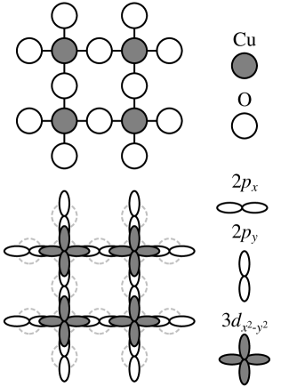
FIG. 1.: Diagram of the CuO planes showing four unit cells and the overlay of the Cu $3d_{x^{2}-y^{2}}$ and O $2p_{x}$ and $2p_{y}$ orbitals. Note that a more realistic picture would show the actual hybrid orbitals of the high-$T_{c}$ CuO planes.

III The Model

In high-$T_{c}$ systems, conduction takes place in the copper-oxygen planes. The unit cell consists of one copper and two oxygen atoms as seen in Fig. 1. The chemistry of these atoms suggest, and band structure calculations confirm, that there is only one orbital on each site that plays a role in this conduction. These are the oxygen $2p_{x}$ or $2p_{y}$ orbitals ($x$ or $y$ depending on which one points to the neighboring copper atoms) and the copper $3d_{x^{2}-y^{2}}$ orbital. The six states must accommodate five electrons in, for example, La₂CuO₄. We shall call this the half-filled band case, for reasons which will become clear later. In La_2-xSr_xCuO₄, they must accommodate $5-x$ electrons, as Sr contributes 1 less electron per unit cell to the CuO planes. The noninteracting model is easily solved.

Let us take creation operators $d^{\dagger}_{\bf r}$, $p^{\dagger}_{{\bf r}1}$, and $p^{\dagger}_{{\bf r}2}$. Then the Hamiltonian is

$${\cal H} = \sum_{\bf r}\varepsilon_{d}d^{\dagger}_{\bf r}d_{\bf r}+\sum_{\bf r}\varepsilon_{p}(p^{\dagger}_{{\bf r}1}p_{{\bf r}1}+p^{\dagger}_{{\bf r}2}p_{{\bf r}2})$$ (4)

$$-t_{pd\sigma}\sum_{\bf r}\left[(d^{\dagger}_{\bf r}p_{{\bf r}1}+p^{\dagger}_{{\bf r}1}d_{\bf r})-(d^{\dagger}_{\bf r}p_{{\bf r}2}+p^{\dagger}_{{\bf r}2}d_{\bf r})\right]$$

$$+t_{pd\sigma}\sum_{\bf r}\left[(d^{\dagger}_{{\bf r}+a\hat{x}}p_{{\bf r}1}+p^{\dagger}_{{\bf r}1}d_{{\bf r}+a\hat{x}})\right.$$

$$~{}~{}~{}~{}~{}~{}~{}~{}~{}~{}~{}\left.-(d^{\dagger}_{{\bf r}+a\hat{y}}p_{{\bf r}2}+p^{\dagger}_{{\bf r}2}d_{{\bf r}+a\hat{y}})\right].$$

Here, $\varepsilon_{d}$ and $\varepsilon_{p}$ are the atomic energies of the two orbitals and

$$t_{pd\sigma}\equiv-\int d^{3}r~{}\psi_{d}({\bf r})~{}\Delta{\cal H}~{}\psi_{py}({\bf r}-a\hat{y})$$ (5)

is the overlap integral of the $3d_{x^{2}-y^{2}}$ orbital and the $2p_{y}$ orbital in the unit cell. $\Delta{\cal H}$ is the difference of the atomic and crystal Hamiltonians. All the other overlaps in our restricted basis set are related to this one by symmetry. The relative signs in the Hamiltonian are important, and are determined by the character of the atomic wavefunctions. The above tight-binding Hamiltonian assumes that the orbitals are orthogonal to each other.

The Bloch wavefunction is now defined by

$$\psi_{\bf k} = \frac{1}{\sqrt{N_{c}}}\sum_{\bf r}e^{i{\bf k}\cdot{\bf r}}$$ (7)

$$\times\left[u_{1}~{}p^{\dagger}_{{\bf r}1}({\bf k})+u_{2}~{}p^{\dagger}_{{\bf r}2}({\bf k})+u_{3}~{}d^{\dagger}_{\bf r}({\bf k})\right]\left|0\right>,$$

with the $u_{i}({\bf k})$ still to be determined. The matrix elements of ${\cal H}$ are

$$\left<\psi^{*}_{\bf k}|{\cal H}|\psi_{{\bf k}^{\prime}}\right>=\delta_{{\bf k},{\bf k}^{\prime}}\sum_{i,j}~{}h_{ij}({\bf k})~{}u^{*}_{i}({\bf k})~{}u_{j}({\bf k}),$$ (8)

with

$$h_{ij}({\bf k})=$$ (9)

$$\left(\begin{array}[]{ccc}\varepsilon_{p}&0&t_{pd\sigma}(\text{-}1+e^{ik_{y}a})\\ 0&\varepsilon_{p}&t_{pd\sigma}(1-e^{ik_{x}a})\\ t_{pd\sigma}(\text{-}1+e^{-ik_{y}a})&t_{pd\sigma}(1-e^{-ik_{x}a})&\varepsilon_{d}\end{array}\right)$$ (13)

as may be verified by a simple calculation. The secular equation to determine the eigenvalues $\varepsilon({\bf k})$ at a given wavevector is

$$\left|h_{ij}({\bf k})-\varepsilon({\bf k})\right|=0,$$ (14)

which takes the form

$$(\varepsilon_{p}-\varepsilon({\bf k}))\left[(\varepsilon_{p}-\varepsilon({\bf k}))(\varepsilon_{d}-\varepsilon({\bf k}))-4t_{pd\sigma}^{2}\sin^{2}{\left(\frac{k_{x}a}{2}\right)}\right.$$ (15)

$$~{}~{}~{}~{}~{}~{}~{}~{}~{}~{}~{}~{}~{}~{}\left.-4t_{pd\sigma}^{2}\sin^{2}{\left(\frac{k_{x}a}{2}\right)}\right]=0.$$ (16)

There are three solutions to this equation, which we shall call $\varepsilon_{n}({\bf k})$, $\varepsilon_{+}({\bf k})$, and $\varepsilon_{-}({\bf k})$. They are

$$\varepsilon_{n}({\bf k}) = \varepsilon_{p},$$ (17)

$$\varepsilon_{\pm}({\bf k}) = \frac{\varepsilon_{p}+\varepsilon_{d}}{2}\pm\frac{1}{2}\left[(\varepsilon_{d}-\varepsilon_{p})^{2}+16t_{pd\sigma}^{2}\sin^{2}{\left(\frac{k_{x}a}{2}\right)}\right.$$ (19)

$$~{}~{}~{}~{}~{}~{}~{}~{}~{}~{}~{}~{}~{}~{}~{}~{}\left.+16t_{pd\sigma}^{2}\sin^{2}{\left(\frac{k_{x}a}{2}\right)}\right]^{1/2}.$$

We see that the band corresponding to $\varepsilon_{n}({\bf k})$ is completely flat. It has no amplitude on the Cu-atoms and can be thought of as a nonbonding orbital. $\varepsilon_{-}({\bf k})$ has dispersion which reaches downward from the atomic energies and is a bonding orbital. $\varepsilon_{+}({\bf k})$ has dispersion which reaches upward from the atomic energies and is an antibonding orbital. It is generally found that $\varepsilon_{p}\approx\varepsilon_{d}$. This leads to the very strong hybridization between copper and oxygen which is characteristic of the high-$T_{c}$ materials and distinguishes them, chemically, from most other transition-metal oxides. The two energies lie about $3.2$ eV below the Fermi energy. (We shall not attempt to assign precise values to these bare parameters, since the observable parameters are those of the effective model to be derived below. They are the important ones, and they are best taken from experiment.) With $t_{pd\sigma}\approx 1.80$ eV, only the antibonding band crosses the Fermi energy. At the Fermi energy, the wavefunctions have substantial weight at both copper and oxygen sites.

With interaction, we must add a term

$${\cal H}_{\text{int}}=U_{d}\sum_{\bf r}n_{d{\bf r}\uparrow}n_{d{\bf r}\downarrow}+U_{p}\sum_{{\bf r}i}n_{p{\bf r}i\uparrow}n_{p{\bf r}i\downarrow}.$$ (20)

Here the sum runs over all atoms in the plane, and the interaction is approximated to be local; only electrons on the same atom interact. Theories of high-temperature superconductivity based on charge fluctuation-mediated attractions go beyond this approximation by including longer-range terms, particularly interactions between electrons on neighboring copper and oxygen atoms. These interactions are not so important for the magnetic mechanisms which are the subject of this paper.

Since the parameter $U_{d}$ is large, ($\sim 10$ eV) we may expect a considerable revision of the energy levels of the noninteracting problem to take place. In the ground state of the half-filled band case, the copper orbital will have essentially only one electron, since the addition of a second would cost this very large amount of energy. This leads to an insulating state because any flow of charge would require a real change of the occupations from their base values of one per copper and two per oxygen. Such a state is in fact observed in La₂CuO₄. It is also a magnetic state, in the sense that every copper atom has spin one-half. (The atomic configuration is $3d^{9}$.)

$U_{p}$ is smaller than $U_{d}$, but large enough that holes added to the half-filled band state go predominantly to the oxygen sites. Each such site has then also a spin one-half. It was shown by Zhang and Rice [28] that these oxygen spins pair with the copper spins to form a spin singlet. This is the entity which moves from unit cell to unit cell. It produces metallic conduction, as it has a charge of $-1$ relative to the rest of the lattice. It also has a spin of zero, while the other cells have spin one-half because of their unpaired copper spins. The Hamiltonian for these particles is

$${\cal H}_{\text{ZR}} = -t\sum_{{\bf r},\mathchoice{{\hbox{\boldmath$\displaystyle\delta$}}}{{\hbox{\boldmath$\textstyle\delta$}}}{{\hbox{\boldmath$\scriptstyle\delta$}}}{{\hbox{\boldmath$\scriptscriptstyle\delta$}}},\sigma}c^{\dagger}_{{\bf r},\sigma}c_{{\bf r}+\mathchoice{{\hbox{\boldmath$\displaystyle\delta$}}}{{\hbox{\boldmath$\textstyle\delta$}}}{{\hbox{\boldmath$\scriptstyle\delta$}}}{{\hbox{\boldmath$\scriptscriptstyle\delta$}}},\sigma}-t^{\prime}\sum_{{\bf r},\mathchoice{{\hbox{\boldmath$\displaystyle\gamma$}}}{{\hbox{\boldmath$\textstyle\gamma$}}}{{\hbox{\boldmath$\scriptstyle\gamma$}}}{{\hbox{\boldmath$\scriptscriptstyle\gamma$}}},\sigma}c^{\dagger}_{{\bf r},\sigma}c_{{\bf r}+\mathchoice{{\hbox{\boldmath$\displaystyle\gamma$}}}{{\hbox{\boldmath$\textstyle\gamma$}}}{{\hbox{\boldmath$\scriptstyle\gamma$}}}{{\hbox{\boldmath$\scriptscriptstyle\gamma$}}},\sigma}$$ (22)

$$+U\sum_{\bf r}n_{{\bf r}\uparrow}n_{{\bf r}\downarrow}.$$

We refer the reader to Ref. [28] for the details of the derivation. Here $c_{{\bf r}\sigma}$ creates a hole and ${\bf r}$ refers to the position of a unit cell, not an atom, and $\textstyle\delta$ and $\textstyle\gamma$ are nearest-neighbor and next-nearest-neighbor vectors, respectively, of the square lattice of unit cells. This Hamiltonian is known as the single-band Hubbard Hamiltonian. It has received a great deal of attention in connection with the high-$T_{c}$ problem. Our aim here is not to review this work, but to do the simplest calculations which are relevant to superconductivity in a certain limit of the model, namely the limit $U>>t,U>>t^{\prime}$. We shall assume that $t$ and $t^{\prime}$ are of the same order of magnitude.

The appropriate method in this limit is perturbative, in that the interaction term ${\cal H}_{\text{int}}$ is taken as the unperturbed Hamiltonian. We have that

$${\cal H}_{\text{int}}=U\sum_{\bf r}n_{{\bf r}\uparrow}n_{{\bf r}\downarrow},$$ (23)

and we wish to solve

$${\cal H}_{\text{int}}\Psi=E\Psi,$$ (24)

to get started. Since ${\cal H}_{\text{int}}$ simply counts the number of doubly-occupied sites, however, the basis of wavefunctions in configuration space (where the occupation of each site is specified) is already diagonal. The eigenvalues are just $0$, $U$, $2U$, and so on, corresponding to $0$, $1$, $2$, etc., doubly-occupied sites. Each eigenvalue is very highly degenerate. Since our interest is in the low energy states, let us concentrate on the subspace with no doubly-occupied sites, with an unperturbed energy of zero.

Now turn on the perturbation, which is

$$\sum_{{\bf k}s}\varepsilon_{\bf k}n_{{\bf k}s}.$$ (25)

The effect of this operator on a state in configuration space is to move one electron from one site to a nearby site. In acting on a state with no doubly-occupied sites, it may, for example, move an electron to a site which is already singly-occupied, thereby increasing the number of doubly-occupied sites by one. The kinetic energy operator has the effect of mixing the different subspaces. We shall take this into account in the following way. If an arbitrary wavefunction $\Psi$ is written in configuration space, then it may be decomposed as

$$\Psi=\Psi_{0}+\Psi_{1}+\Psi_{2}+\ldots,$$ (26)

where $\Psi_{0}$ has no doubly-occupied sites, $\Psi_{1}$ has one doubly-occupied site, and so on.

The Schrödinger equation may then be written as

$$\left(\begin{array}[]{cc}\begin{array}[]{ccc}{\cal H}_{00}&{\cal H}_{01}&0\\ {\cal H}_{10}&{\cal H}_{11}&{\cal H}_{12}\\ 0&{\cal H}_{21}&{\cal H}_{22}\end{array}&\ldots\\ \vdots&\ddots\end{array}\right)\left(\begin{array}[]{c}\Psi_{0}\\ \Psi_{1}\\ \Psi_{2}\\ \vdots\end{array}\right)=E\left(\begin{array}[]{c}\Psi_{0}\\ \Psi_{1}\\ \Psi_{2}\\ \vdots\end{array}\right).$$ (27)

Here the $\Psi$ are as defined above, and ${\cal H}_{nn^{\prime}}$ is the part of the Hamiltonian which acts only on a state with $n^{\prime}$ doubly-occupied sites and produces a state with exactly $n$ doubly-occupied sites. This Schrödinger equation is still completely general. If $U$ is large enough, and we are interested only in the low-lying states, we may neglect $\Psi_{2}$, and all states with more than two doubly-occupied sites. Then the first two equations are

$${\cal H}_{00}\Psi_{0}+{\cal H}_{01}\Psi_{1} = E\Psi_{0},$$ (28)

$${\cal H}_{10}\Psi_{0}+{\cal H}_{11}\Psi_{1} = E\Psi_{1}.$$ (29)

Substituting the second equation into the first, we find

$${\cal H}_{00}\Psi_{0}+{\cal H}_{01}(E-{\cal H}_{11})^{-1}{\cal H}_{10}\Psi_{0}=E\Psi_{0}.$$ (30)

The second term on the left-hand side has the following structure. ${\cal H}_{10}\Psi_{0}$ is a state with exactly one doubly-occupied site. Its energy is therefore $U$, with corrections of order $t$ or $t^{\prime}$. ${\cal H}_{11}$ acting on this state gives $U$ to the approximation in which we are interested, and we may write the entire equation as

$${\cal H}_{00}\Psi_{0}-\frac{1}{U}{\cal H}_{01}{\cal H}_{10}\Psi_{0}=E\Psi_{0}.$$ (31)

We have then a new Schrödinger equation to solve, which may be written as

$${\cal H}_{\text{eff}}\Psi_{0}=E\Psi_{0},$$ (32)

with

$${\cal H}_{\text{eff}}={\cal H}_{00}-\frac{1}{U}{\cal H}_{01}{\cal H}_{10}.$$ (33)

In this equation, the second term represents virtual processes in which a doubly-occupied site is first created, then destroyed. In second order perturbation theory (order $t^{2}$), these processes affect the energies of the lowest energy states and break the degeneracy of the lowest level. Note that ${\cal H}_{00}$ also has kinetic energy terms if the band is less than half filled, as it is possible then to move electrons from one singly-occupied site to another, creating no doubly-occupied sites. Explicitly, the various operators have the form

$${\cal H}_{10} = -t\sum_{{\bf r},\mathchoice{{\hbox{\boldmath$\displaystyle\delta$}}}{{\hbox{\boldmath$\textstyle\delta$}}}{{\hbox{\boldmath$\scriptstyle\delta$}}}{{\hbox{\boldmath$\scriptscriptstyle\delta$}}},\sigma}n_{{\bf r},-\sigma}c^{\dagger}_{{\bf r},\sigma}c_{{\bf r}+\mathchoice{{\hbox{\boldmath$\displaystyle\delta$}}}{{\hbox{\boldmath$\textstyle\delta$}}}{{\hbox{\boldmath$\scriptstyle\delta$}}}{{\hbox{\boldmath$\scriptscriptstyle\delta$}}},\sigma}(1-n_{{\bf r}+\mathchoice{{\hbox{\boldmath$\displaystyle\delta$}}}{{\hbox{\boldmath$\textstyle\delta$}}}{{\hbox{\boldmath$\scriptstyle\delta$}}}{{\hbox{\boldmath$\scriptscriptstyle\delta$}}},-\sigma})$$ (35)

$$-t^{\prime}\sum_{{\bf r},\mathchoice{{\hbox{\boldmath$\displaystyle\gamma$}}}{{\hbox{\boldmath$\textstyle\gamma$}}}{{\hbox{\boldmath$\scriptstyle\gamma$}}}{{\hbox{\boldmath$\scriptscriptstyle\gamma$}}},\sigma}n_{{\bf r},-\sigma}c^{\dagger}_{{\bf r},\sigma}c_{{\bf r}+\mathchoice{{\hbox{\boldmath$\displaystyle\gamma$}}}{{\hbox{\boldmath$\textstyle\gamma$}}}{{\hbox{\boldmath$\scriptstyle\gamma$}}}{{\hbox{\boldmath$\scriptscriptstyle\gamma$}}},\sigma}(1-n_{{\bf r}+\mathchoice{{\hbox{\boldmath$\displaystyle\gamma$}}}{{\hbox{\boldmath$\textstyle\gamma$}}}{{\hbox{\boldmath$\scriptstyle\gamma$}}}{{\hbox{\boldmath$\scriptscriptstyle\gamma$}}},-\sigma})$$

$${\cal H}_{01} = -t\sum_{{\bf r},\mathchoice{{\hbox{\boldmath$\displaystyle\delta$}}}{{\hbox{\boldmath$\textstyle\delta$}}}{{\hbox{\boldmath$\scriptstyle\delta$}}}{{\hbox{\boldmath$\scriptscriptstyle\delta$}}},\sigma}(1-n_{{\bf r},-\sigma})c^{\dagger}_{{\bf r},\sigma}c_{{\bf r}+\mathchoice{{\hbox{\boldmath$\displaystyle\delta$}}}{{\hbox{\boldmath$\textstyle\delta$}}}{{\hbox{\boldmath$\scriptstyle\delta$}}}{{\hbox{\boldmath$\scriptscriptstyle\delta$}}},\sigma}n_{{\bf r}+\mathchoice{{\hbox{\boldmath$\displaystyle\delta$}}}{{\hbox{\boldmath$\textstyle\delta$}}}{{\hbox{\boldmath$\scriptstyle\delta$}}}{{\hbox{\boldmath$\scriptscriptstyle\delta$}}},-\sigma}$$ (37)

$$-t^{\prime}\sum_{{\bf r},\mathchoice{{\hbox{\boldmath$\displaystyle\gamma$}}}{{\hbox{\boldmath$\textstyle\gamma$}}}{{\hbox{\boldmath$\scriptstyle\gamma$}}}{{\hbox{\boldmath$\scriptscriptstyle\gamma$}}},\sigma}(1-n_{{\bf r},-\sigma})c^{\dagger}_{{\bf r},\sigma}c_{{\bf r}+\mathchoice{{\hbox{\boldmath$\displaystyle\gamma$}}}{{\hbox{\boldmath$\textstyle\gamma$}}}{{\hbox{\boldmath$\scriptstyle\gamma$}}}{{\hbox{\boldmath$\scriptscriptstyle\gamma$}}},\sigma}n_{{\bf r}+\mathchoice{{\hbox{\boldmath$\displaystyle\gamma$}}}{{\hbox{\boldmath$\textstyle\gamma$}}}{{\hbox{\boldmath$\scriptstyle\gamma$}}}{{\hbox{\boldmath$\scriptscriptstyle\gamma$}}},-\sigma}$$

$${\cal H}_{00} = -t\sum_{{\bf r},\mathchoice{{\hbox{\boldmath$\displaystyle\delta$}}}{{\hbox{\boldmath$\textstyle\delta$}}}{{\hbox{\boldmath$\scriptstyle\delta$}}}{{\hbox{\boldmath$\scriptscriptstyle\delta$}}},\sigma}(1-n_{{\bf r},-\sigma})c^{\dagger}_{{\bf r},\sigma}c_{{\bf r}+\mathchoice{{\hbox{\boldmath$\displaystyle\delta$}}}{{\hbox{\boldmath$\textstyle\delta$}}}{{\hbox{\boldmath$\scriptstyle\delta$}}}{{\hbox{\boldmath$\scriptscriptstyle\delta$}}},\sigma}(1-n_{{\bf r}+\mathchoice{{\hbox{\boldmath$\displaystyle\delta$}}}{{\hbox{\boldmath$\textstyle\delta$}}}{{\hbox{\boldmath$\scriptstyle\delta$}}}{{\hbox{\boldmath$\scriptscriptstyle\delta$}}},-\sigma})$$ (39)

$$-t^{\prime}\sum_{{\bf r},\mathchoice{{\hbox{\boldmath$\displaystyle\gamma$}}}{{\hbox{\boldmath$\textstyle\gamma$}}}{{\hbox{\boldmath$\scriptstyle\gamma$}}}{{\hbox{\boldmath$\scriptscriptstyle\gamma$}}},\sigma}(1-n_{{\bf r},-\sigma})c^{\dagger}_{{\bf r},\sigma}c_{{\bf r}+\mathchoice{{\hbox{\boldmath$\displaystyle\gamma$}}}{{\hbox{\boldmath$\textstyle\gamma$}}}{{\hbox{\boldmath$\scriptstyle\gamma$}}}{{\hbox{\boldmath$\scriptscriptstyle\gamma$}}},\sigma}(1-n_{{\bf r}+\mathchoice{{\hbox{\boldmath$\displaystyle\gamma$}}}{{\hbox{\boldmath$\textstyle\gamma$}}}{{\hbox{\boldmath$\scriptstyle\gamma$}}}{{\hbox{\boldmath$\scriptscriptstyle\gamma$}}},-\sigma})$$

The notation indicates that each nearest-neighbor pair and next-nearest-neighbor pair is counted once and once only in the sum.

Writing the result out in its complete form, we have

$${\cal H}_{\text{eff}} = -t\sum_{{\bf r},\mathchoice{{\hbox{\boldmath$\displaystyle\delta$}}}{{\hbox{\boldmath$\textstyle\delta$}}}{{\hbox{\boldmath$\scriptstyle\delta$}}}{{\hbox{\boldmath$\scriptscriptstyle\delta$}}},\sigma}c_{{\bf r},\sigma}^{\dagger}c_{{\bf r}+\mathchoice{{\hbox{\boldmath$\displaystyle\delta$}}}{{\hbox{\boldmath$\textstyle\delta$}}}{{\hbox{\boldmath$\scriptstyle\delta$}}}{{\hbox{\boldmath$\scriptscriptstyle\delta$}}},\sigma}-t^{\prime}\sum_{{\bf r},\mathchoice{{\hbox{\boldmath$\displaystyle\gamma$}}}{{\hbox{\boldmath$\textstyle\gamma$}}}{{\hbox{\boldmath$\scriptstyle\gamma$}}}{{\hbox{\boldmath$\scriptscriptstyle\gamma$}}},\sigma}c_{{\bf r},\sigma}^{\dagger}c_{{\bf r}+\mathchoice{{\hbox{\boldmath$\displaystyle\gamma$}}}{{\hbox{\boldmath$\textstyle\gamma$}}}{{\hbox{\boldmath$\scriptstyle\gamma$}}}{{\hbox{\boldmath$\scriptscriptstyle\gamma$}}},\sigma}$$ (43)

$$+\frac{J}{2}\sum_{{\bf r},\mathchoice{{\hbox{\boldmath$\displaystyle\delta$}}}{{\hbox{\boldmath$\textstyle\delta$}}}{{\hbox{\boldmath$\scriptstyle\delta$}}}{{\hbox{\boldmath$\scriptscriptstyle\delta$}}}}\left({\bf S}_{\bf r}\cdot{\bf S}_{{\bf r}+\mathchoice{{\hbox{\boldmath$\displaystyle\delta$}}}{{\hbox{\boldmath$\textstyle\delta$}}}{{\hbox{\boldmath$\scriptstyle\delta$}}}{{\hbox{\boldmath$\scriptscriptstyle\delta$}}}}-\frac{1}{4}n_{\bf r}n_{{\bf r}+\mathchoice{{\hbox{\boldmath$\displaystyle\delta$}}}{{\hbox{\boldmath$\textstyle\delta$}}}{{\hbox{\boldmath$\scriptstyle\delta$}}}{{\hbox{\boldmath$\scriptscriptstyle\delta$}}}}\right)$$

$$-\frac{J}{4}\sum_{{\bf r},\mathchoice{{\hbox{\boldmath$\displaystyle\delta$}}}{{\hbox{\boldmath$\textstyle\delta$}}}{{\hbox{\boldmath$\scriptstyle\delta$}}}{{\hbox{\boldmath$\scriptscriptstyle\delta$}}}^{\prime}\neq\mathchoice{{\hbox{\boldmath$\displaystyle\delta$}}}{{\hbox{\boldmath$\textstyle\delta$}}}{{\hbox{\boldmath$\scriptstyle\delta$}}}{{\hbox{\boldmath$\scriptscriptstyle\delta$}}},\sigma}\left(c_{{\bf r}+\mathchoice{{\hbox{\boldmath$\displaystyle\delta$}}}{{\hbox{\boldmath$\textstyle\delta$}}}{{\hbox{\boldmath$\scriptstyle\delta$}}}{{\hbox{\boldmath$\scriptscriptstyle\delta$}}},\sigma}^{\dagger}n_{{\bf r},-\sigma}c_{{\bf r}+\mathchoice{{\hbox{\boldmath$\displaystyle\delta$}}}{{\hbox{\boldmath$\textstyle\delta$}}}{{\hbox{\boldmath$\scriptstyle\delta$}}}{{\hbox{\boldmath$\scriptscriptstyle\delta$}}}^{\prime},\sigma}\right.$$

$$~{}~{}~{}~{}~{}~{}~{}~{}~{}~{}~{}~{}~{}\left.+c_{{\bf r}+\mathchoice{{\hbox{\boldmath$\displaystyle\delta$}}}{{\hbox{\boldmath$\textstyle\delta$}}}{{\hbox{\boldmath$\scriptstyle\delta$}}}{{\hbox{\boldmath$\scriptscriptstyle\delta$}}},\sigma}^{\dagger}c_{{\bf r},-\sigma}^{\dagger}c_{{\bf r}+\mathchoice{{\hbox{\boldmath$\displaystyle\delta$}}}{{\hbox{\boldmath$\textstyle\delta$}}}{{\hbox{\boldmath$\scriptstyle\delta$}}}{{\hbox{\boldmath$\scriptscriptstyle\delta$}}}^{\prime},-\sigma}c_{{\bf r},\sigma}\right).$$

This rather complicated Hamiltonian can be separated into three physically quite distinct parts. The first term is a hoping term of the usual kind. An electron hops from the site ${\bf r}+\mathchoice{{\hbox{\boldmath$\displaystyle\delta$}}}{{\hbox{\boldmath$\textstyle\delta$}}}{{\hbox{\boldmath$\scriptstyle\delta$}}}{{\hbox{\boldmath$\scriptscriptstyle\delta$}}}$ to the site ${\bf r}$. The only point which must be borne in mind is that no doubly-occupied sites can be created in this process. This kinetic energy term is formally of order $t$. This is the leading term in an expansion in the small parameter $t/U$. However, the constraint of no doubly-occupied sites means that only “holes” (vacant sites) can move. Thus, the contribution of this term to the energy is proportional to the doping level. If we call the density of vacant sites $\delta$, then the total contribution of this term to the energy is of order $z\delta t$, where $z$ is the coordination number. ($z=4$ for the square lattice). The next term is a spin-spin interaction. It lowers the energy of antiferromagnetic spin configurations. The contribution of this term to the total energy is proportional to $z(1-\delta)J\sim 4z(1-\delta)t^{2}/U$. The final group of terms consists of the three-site terms, which represent a kind of induced kinetic energy through virtual processes. Their contribution to the energy is of order $z^{2}\delta J$. In the high-$T_{c}$ materials, we normally have $J/t\approx 1/3$, and $\delta$ ranges from $0.0$ to $0.4$. As a function of $\delta$, therefore, we expect the spin-spin interaction to be the dominant term at very small $\delta$, while at moderate values of $\delta$, perhaps $\delta\approx 0.1$, the other two terms will start to become important, based on this simple analysis. In fact, which terms are important depends a good deal on the property of the system in which we are interested.

IV The Dilute Limit

The $t$-$J$ model has strong support as a description of the low-lying energy states of the doped CuO₂ planes in the high-temperature superconductors. Such an important model must be investigated over its full range of parameters, not only for the sake of understanding a model which is interesting in and of itself, but also for the purpose of gaining insight into the various trends of the model as its many variables change from one area of parameter space to another. In other words, such a wide-range investigation of the $t$-$J$ model could link nonphysical, yet soluble limits of the model to more physical, insoluble regions. In this spirit of identifying trends, we present in this section an analytical solution to the dilute or low spin-density limit. The basic $t$-$J$ model will first be considered, followed by the model with the addition of three-site terms [29] and next-nearest-neighbor hopping. Justification for this “extended” $t$-$J$ model is made below.

A The basic $t$-$J$ model

Consider two spins, one up and one down, on a square, two-dimensional lattice of $N_{s}$ sites. The goal is to find the ground state of the system satisfying the Schrödinger equation

$$\tilde{\cal H}_{tJ}\left|\psi\right>=E\left|\psi\right>,$$ (44)

where $E$ is the binding energy of the two spins. These spins interact as described by the “traditional” $t$-$J$ model Eq. (43) which may be written as:

$${\cal H}_{tJ} = -t\sum_{{\bf r},\mathchoice{{\hbox{\boldmath$\displaystyle\delta$}}}{{\hbox{\boldmath$\textstyle\delta$}}}{{\hbox{\boldmath$\scriptstyle\delta$}}}{{\hbox{\boldmath$\scriptscriptstyle\delta$}}},\sigma}c_{{\bf r},\sigma}^{\dagger}c_{{\bf r}+\mathchoice{{\hbox{\boldmath$\displaystyle\delta$}}}{{\hbox{\boldmath$\textstyle\delta$}}}{{\hbox{\boldmath$\scriptstyle\delta$}}}{{\hbox{\boldmath$\scriptscriptstyle\delta$}}},\sigma}$$ (46)

$$-\frac{J}{4}\sum_{{\bf r},\mathchoice{{\hbox{\boldmath$\displaystyle\delta$}}}{{\hbox{\boldmath$\textstyle\delta$}}}{{\hbox{\boldmath$\scriptstyle\delta$}}}{{\hbox{\boldmath$\scriptscriptstyle\delta$}}},\sigma}(n_{{\bf r},-\sigma}n_{{\bf r}+\mathchoice{{\hbox{\boldmath$\displaystyle\delta$}}}{{\hbox{\boldmath$\textstyle\delta$}}}{{\hbox{\boldmath$\scriptstyle\delta$}}}{{\hbox{\boldmath$\scriptscriptstyle\delta$}}},\sigma}+c_{{\bf r}+\mathchoice{{\hbox{\boldmath$\displaystyle\delta$}}}{{\hbox{\boldmath$\textstyle\delta$}}}{{\hbox{\boldmath$\scriptstyle\delta$}}}{{\hbox{\boldmath$\scriptscriptstyle\delta$}}},\sigma}^{\dagger}c_{{\bf r},-\sigma}^{\dagger}c_{{\bf r}+\mathchoice{{\hbox{\boldmath$\displaystyle\delta$}}}{{\hbox{\boldmath$\textstyle\delta$}}}{{\hbox{\boldmath$\scriptstyle\delta$}}}{{\hbox{\boldmath$\scriptscriptstyle\delta$}}},-\sigma}c_{{\bf r},\sigma}),$$

where summations are over the $N_{s}$ sites ${\bf r}$, the four nearest-neighbor sites $\textstyle\delta$, and spin up and down $\sigma$. The $J$-term is written in the above form for convenience in comparing it with additional terms later. To find the ground state of the system, the following pair wavefunction form is used:

$$\left|\psi\right>=\sum_{{\bf r}_{1},{\bf r}_{2}}a({\bf r}_{1}-{\bf r}_{2})c_{{\bf r}_{1}\uparrow}^{\dagger}c_{{\bf r}_{2}\downarrow}^{\dagger}\left|0\right>,$$ (47)

where the solution entails finding $a({\bf r})$ at all ${\bf r}$. Before this is done, it should be noted that, although the $t$-$J$ model implicitly includes the restriction of no-doubly-occupied sites, the given form in Eq. (46) will not reflect this constraint unless an on-site repulsion term is added as

$$\tilde{\cal H}_{tJ} = {\cal H}_{tJ}+{\cal H}_{V_{0}},$$ (48)

$${\cal H}_{V_{0}} = V_{0}\sum_{\bf r}n_{{\bf r}\uparrow}n_{{\bf r}\downarrow},$$ (49)

where the limit $V_{0}\rightarrow\infty$ will yield the desired constraint $a({\bf r}=0)=0$. In other words, the probability of finding the pair on the same site will be zero as required. This added term is, of course, identical to the Hubbard $U$-term of Eq. (23).

Substitution of Eqs. (47) and (49) into Eq. (44) and appropriate relabeling of summation variables reduce the problem to the following equation in $a$:

$$-2t\sum_{\mathchoice{{\hbox{\boldmath$\displaystyle\delta$}}}{{\hbox{\boldmath$\textstyle\delta$}}}{{\hbox{\boldmath$\scriptstyle\delta$}}}{{\hbox{\boldmath$\scriptscriptstyle\delta$}}}}a({\bf r}+\mathchoice{{\hbox{\boldmath$\displaystyle\delta$}}}{{\hbox{\boldmath$\textstyle\delta$}}}{{\hbox{\boldmath$\scriptstyle\delta$}}}{{\hbox{\boldmath$\scriptscriptstyle\delta$}}})-\frac{J}{2}\sum_{\mathchoice{{\hbox{\boldmath$\displaystyle\delta$}}}{{\hbox{\boldmath$\textstyle\delta$}}}{{\hbox{\boldmath$\scriptstyle\delta$}}}{{\hbox{\boldmath$\scriptscriptstyle\delta$}}}}(a({\bf r})-a({\bf r}-2\mathchoice{{\hbox{\boldmath$\displaystyle\delta$}}}{{\hbox{\boldmath$\textstyle\delta$}}}{{\hbox{\boldmath$\scriptstyle\delta$}}}{{\hbox{\boldmath$\scriptscriptstyle\delta$}}}))\delta_{{\bf r},\mathchoice{{\hbox{\boldmath$\displaystyle\delta$}}}{{\hbox{\boldmath$\textstyle\delta$}}}{{\hbox{\boldmath$\scriptstyle\delta$}}}{{\hbox{\boldmath$\scriptscriptstyle\delta$}}}}$$ (50)

$$+V_{0}a({\bf r})\delta_{{\bf r},0}=Ea({\bf r}),$$ (51)

where ${\bf r}_{1}$ and ${\bf r}_{2}$ are fixed, and the relative coordinate ${\bf r}={\bf r}_{1}-{\bf r}_{2}$ is used. Using the following relations:

$$a({\bf k}) = \frac{1}{N_{s}}\sum_{\bf r}e^{-i{\bf k}\cdot{\bf r}}a({\bf r}),$$ (52)

$$a({\bf r}) = \sum_{\bf k}e^{i{\bf k}\cdot{\bf r}}a({\bf k}),$$ (53)

the Fourier transform of Eq. (51) is taken, and solving for $a({\bf k})$ yields

$$a({\bf k}) = \frac{J}{2N_{s}}\sum_{\mathchoice{{\hbox{\boldmath$\displaystyle\delta$}}}{{\hbox{\boldmath$\textstyle\delta$}}}{{\hbox{\boldmath$\scriptstyle\delta$}}}{{\hbox{\boldmath$\scriptscriptstyle\delta$}}}}a(\mathchoice{{\hbox{\boldmath$\displaystyle\delta$}}}{{\hbox{\boldmath$\textstyle\delta$}}}{{\hbox{\boldmath$\scriptstyle\delta$}}}{{\hbox{\boldmath$\scriptscriptstyle\delta$}}})\frac{\cos{{\bf k}\cdot\mathchoice{{\hbox{\boldmath$\displaystyle\delta$}}}{{\hbox{\boldmath$\textstyle\delta$}}}{{\hbox{\boldmath$\scriptstyle\delta$}}}{{\hbox{\boldmath$\scriptscriptstyle\delta$}}}}}{\varepsilon({\bf k})-E/2}$$ (55)

$$-\frac{V_{0}}{2N_{s}}a(0)\frac{1}{\varepsilon({\bf k})-E/2},$$

where $\varepsilon({\bf k})=-2t(\cos k_{x}+\cos k_{y})$ is the tight-binding energy dispersion. The inverse Fourier transform of Eq. (55) is then taken, resulting in the following:

$$a({\bf r}) = \frac{J}{2}\sum_{\mathchoice{{\hbox{\boldmath$\displaystyle\delta$}}}{{\hbox{\boldmath$\textstyle\delta$}}}{{\hbox{\boldmath$\scriptstyle\delta$}}}{{\hbox{\boldmath$\scriptscriptstyle\delta$}}}}a(\mathchoice{{\hbox{\boldmath$\displaystyle\delta$}}}{{\hbox{\boldmath$\textstyle\delta$}}}{{\hbox{\boldmath$\scriptstyle\delta$}}}{{\hbox{\boldmath$\scriptscriptstyle\delta$}}})\frac{1}{N_{s}}\sum_{\bf k}\frac{e^{i{\bf k}\cdot{\bf r}}\cos{{\bf k}\cdot\mathchoice{{\hbox{\boldmath$\displaystyle\delta$}}}{{\hbox{\boldmath$\textstyle\delta$}}}{{\hbox{\boldmath$\scriptstyle\delta$}}}{{\hbox{\boldmath$\scriptscriptstyle\delta$}}}}}{\varepsilon({\bf k})-E/2}$$ (57)

$$-\frac{V_{0}}{2}a(0)\frac{1}{N_{s}}\sum_{\bf k}\frac{e^{i{\bf k}\cdot{\bf r}}}{\varepsilon({\bf k})-E/2}.$$

$a(0)$ can be found self-consistently from Eq. (57) to be

$$a(0) = \frac{J}{V_{0}}\frac{I_{1}}{I_{0}+2/V_{0}}\sum_{\mathchoice{{\hbox{\boldmath$\displaystyle\delta$}}}{{\hbox{\boldmath$\textstyle\delta$}}}{{\hbox{\boldmath$\scriptstyle\delta$}}}{{\hbox{\boldmath$\scriptscriptstyle\delta$}}}}a(\mathchoice{{\hbox{\boldmath$\displaystyle\delta$}}}{{\hbox{\boldmath$\textstyle\delta$}}}{{\hbox{\boldmath$\scriptstyle\delta$}}}{{\hbox{\boldmath$\scriptscriptstyle\delta$}}}),$$ (58)

$$I_{0} \equiv \frac{1}{N_{s}}\sum_{\bf k}\frac{1}{\varepsilon({\bf k})-E/2},$$ (59)

$$I_{1} \equiv \frac{1}{N_{s}}\sum_{\bf k}\frac{\cos{k_{x}}}{\varepsilon({\bf k})-E/2}.$$ (60)

Substituting the solution of $a(0)$ back into Eq. (57) then yields the following:

$$a({\bf r}) = \frac{J}{2}\sum_{\mathchoice{{\hbox{\boldmath$\displaystyle\delta$}}}{{\hbox{\boldmath$\textstyle\delta$}}}{{\hbox{\boldmath$\scriptstyle\delta$}}}{{\hbox{\boldmath$\scriptscriptstyle\delta$}}}}a(\mathchoice{{\hbox{\boldmath$\displaystyle\delta$}}}{{\hbox{\boldmath$\textstyle\delta$}}}{{\hbox{\boldmath$\scriptstyle\delta$}}}{{\hbox{\boldmath$\scriptscriptstyle\delta$}}})$$ (62)

$$\times\frac{1}{N_{s}}\sum_{\bf k}\frac{e^{i{\bf k}\cdot{\bf r}}\left(\cos{{\bf k}\cdot\mathchoice{{\hbox{\boldmath$\displaystyle\delta$}}}{{\hbox{\boldmath$\textstyle\delta$}}}{{\hbox{\boldmath$\scriptstyle\delta$}}}{{\hbox{\boldmath$\scriptscriptstyle\delta$}}}}-I_{1}/(I_{0}+2/V_{0})\right)}{\varepsilon({\bf k})-E/2}.$$

It can be seen readily at this point that $a(-{\bf r})=a({\bf r})$ as should be expected from the symmetric form of the wavefunction chosen in Eq. (47) above. The four nearest-neighbor $a(\mathchoice{{\hbox{\boldmath$\displaystyle\delta$}}}{{\hbox{\boldmath$\textstyle\delta$}}}{{\hbox{\boldmath$\scriptstyle\delta$}}}{{\hbox{\boldmath$\scriptscriptstyle\delta$}}})$’s can now be found. Letting $\mathchoice{{\hbox{\boldmath$\displaystyle\delta$}}}{{\hbox{\boldmath$\textstyle\delta$}}}{{\hbox{\boldmath$\scriptstyle\delta$}}}{{\hbox{\boldmath$\scriptscriptstyle\delta$}}}_{1}=(1,0)$, $\mathchoice{{\hbox{\boldmath$\displaystyle\delta$}}}{{\hbox{\boldmath$\textstyle\delta$}}}{{\hbox{\boldmath$\scriptstyle\delta$}}}{{\hbox{\boldmath$\scriptscriptstyle\delta$}}}_{2}=(0,1)$, $\mathchoice{{\hbox{\boldmath$\displaystyle\delta$}}}{{\hbox{\boldmath$\textstyle\delta$}}}{{\hbox{\boldmath$\scriptstyle\delta$}}}{{\hbox{\boldmath$\scriptscriptstyle\delta$}}}_{3}=(-1,0)$, and $\mathchoice{{\hbox{\boldmath$\displaystyle\delta$}}}{{\hbox{\boldmath$\textstyle\delta$}}}{{\hbox{\boldmath$\scriptstyle\delta$}}}{{\hbox{\boldmath$\scriptscriptstyle\delta$}}}_{4}=(0,-1)$, the even symmetry of $a({\bf r})$ requires that $a(\mathchoice{{\hbox{\boldmath$\displaystyle\delta$}}}{{\hbox{\boldmath$\textstyle\delta$}}}{{\hbox{\boldmath$\scriptstyle\delta$}}}{{\hbox{\boldmath$\scriptscriptstyle\delta$}}}_{3})=a(\mathchoice{{\hbox{\boldmath$\displaystyle\delta$}}}{{\hbox{\boldmath$\textstyle\delta$}}}{{\hbox{\boldmath$\scriptstyle\delta$}}}{{\hbox{\boldmath$\scriptscriptstyle\delta$}}}_{1})$ and $a(\mathchoice{{\hbox{\boldmath$\displaystyle\delta$}}}{{\hbox{\boldmath$\textstyle\delta$}}}{{\hbox{\boldmath$\scriptstyle\delta$}}}{{\hbox{\boldmath$\scriptscriptstyle\delta$}}}_{4})=a(\mathchoice{{\hbox{\boldmath$\displaystyle\delta$}}}{{\hbox{\boldmath$\textstyle\delta$}}}{{\hbox{\boldmath$\scriptstyle\delta$}}}{{\hbox{\boldmath$\scriptscriptstyle\delta$}}}_{2})$. Solving for both $a(\mathchoice{{\hbox{\boldmath$\displaystyle\delta$}}}{{\hbox{\boldmath$\textstyle\delta$}}}{{\hbox{\boldmath$\scriptstyle\delta$}}}{{\hbox{\boldmath$\scriptscriptstyle\delta$}}}_{1})$ and $a(\mathchoice{{\hbox{\boldmath$\displaystyle\delta$}}}{{\hbox{\boldmath$\textstyle\delta$}}}{{\hbox{\boldmath$\scriptstyle\delta$}}}{{\hbox{\boldmath$\scriptscriptstyle\delta$}}}_{2})$ self-consistently in Eq. (62) results in $a(\mathchoice{{\hbox{\boldmath$\displaystyle\delta$}}}{{\hbox{\boldmath$\textstyle\delta$}}}{{\hbox{\boldmath$\scriptstyle\delta$}}}{{\hbox{\boldmath$\scriptscriptstyle\delta$}}}_{2})=\pm a(\mathchoice{{\hbox{\boldmath$\displaystyle\delta$}}}{{\hbox{\boldmath$\textstyle\delta$}}}{{\hbox{\boldmath$\scriptstyle\delta$}}}{{\hbox{\boldmath$\scriptscriptstyle\delta$}}}_{1})$. Thus, two solutions for $a({\bf r})$ are obtained:

$$a_{s}({\bf r}) = Ja(\mathchoice{{\hbox{\boldmath$\displaystyle\delta$}}}{{\hbox{\boldmath$\textstyle\delta$}}}{{\hbox{\boldmath$\scriptstyle\delta$}}}{{\hbox{\boldmath$\scriptscriptstyle\delta$}}}_{1})\frac{1}{N_{s}}\sum_{\bf k}e^{i{\bf k}\cdot{\bf r}}$$ (64)

$$\times\frac{\left(\cos{k_{x}}+\cos{k_{y}}-2I_{1}/(I_{0}+2/V_{0})\right)}{\varepsilon({\bf k})-E/2}$$

$$a_{d}({\bf r}) = Ja(\mathchoice{{\hbox{\boldmath$\displaystyle\delta$}}}{{\hbox{\boldmath$\textstyle\delta$}}}{{\hbox{\boldmath$\scriptstyle\delta$}}}{{\hbox{\boldmath$\scriptscriptstyle\delta$}}}_{1})\frac{1}{N_{s}}\sum_{\bf k}e^{i{\bf k}\cdot{\bf r}}\frac{\left(\cos{k_{x}}-\cos{k_{y}}\right)}{\varepsilon({\bf k})-E/2},$$ (65)

where Eqs. (64) and (65) correspond to an extended $s$-wave ($s_{x^{2}+y^{2}}$) solution and a $d$-wave ($d_{x^{2}-y^{2}}$) solution, respectively.

The $d_{x^{2}-y^{2}}$-wave solution in Eq. (65) has no dependence on $V_{0}$, and it can be seen by symmetry alone that $a_{d}(0)=0$; that is, there is no double-occupancy. The $s$-wave solution in Eq. (64) also obtains this constraint upon letting the on-site repulsion $V_{0}$ become infinite:

$$\lim_{V_{0}\rightarrow\infty}a_{s}({\bf r}) = Ja(\mathchoice{{\hbox{\boldmath$\displaystyle\delta$}}}{{\hbox{\boldmath$\textstyle\delta$}}}{{\hbox{\boldmath$\scriptstyle\delta$}}}{{\hbox{\boldmath$\scriptscriptstyle\delta$}}}_{1})\frac{1}{N_{s}}\sum_{\bf k}e^{i{\bf k}\cdot{\bf r}}$$ (67)

$$\times\frac{\left(\cos{k_{x}}+\cos{k_{y}}-2I_{1}/I_{0}\right)}{\varepsilon({\bf k})-E/2},$$

where it can be seen that $a_{s}(0)=0$ by using the definitions of $I_{0}$ and $I_{1}$ in Eqs. (59) and (60) above. Finally, in the thermodynamic limit ($N_{s}\rightarrow\infty$), the sums over ${\bf k}$ become integrals over $d{\bf k}$, and the solutions to the “traditional” $t$-$J$ model in the dilute limit of one pair of spins become

$$a_{s}({\bf r}) = Ja(\mathchoice{{\hbox{\boldmath$\displaystyle\delta$}}}{{\hbox{\boldmath$\textstyle\delta$}}}{{\hbox{\boldmath$\scriptstyle\delta$}}}{{\hbox{\boldmath$\scriptscriptstyle\delta$}}}_{1})\frac{1}{(2\pi)^{2}}\int d{\bf k}e^{i{\bf k}\cdot{\bf r}}$$ (69)

$$\times\frac{\left(\cos{k_{x}}+\cos{k_{y}}-2I_{1}/I_{0}\right)}{\varepsilon({\bf k})-E/2},$$

$$a_{d}({\bf r}) = Ja(\mathchoice{{\hbox{\boldmath$\displaystyle\delta$}}}{{\hbox{\boldmath$\textstyle\delta$}}}{{\hbox{\boldmath$\scriptstyle\delta$}}}{{\hbox{\boldmath$\scriptscriptstyle\delta$}}}_{1})\frac{1}{(2\pi)^{2}}\int d{\bf k}e^{i{\bf k}\cdot{\bf r}}$$ (71)

$$\times\frac{\left(\cos{k_{x}}-\cos{k_{y}}\right)}{\varepsilon({\bf k})-E/2},$$

$$I_{0} = \frac{1}{(2\pi)^{2}}\int d{\bf k}\frac{1}{\varepsilon({\bf k})-E/2},$$ (72)

$$I_{1} = \frac{1}{(2\pi)^{2}}\int d{\bf k}\frac{\cos{k_{x}}}{\varepsilon({\bf k})-E/2},$$ (73)

where integration is over the full Brillouin zone: $k_{x}=-\pi$ to $\pi$ and $k_{y}=-\pi$ to $\pi$.

Of some interest is the critical value of $J$ at which there is a bound state for each solution. Letting ${\bf r}=\mathchoice{{\hbox{\boldmath$\displaystyle\delta$}}}{{\hbox{\boldmath$\textstyle\delta$}}}{{\hbox{\boldmath$\scriptstyle\delta$}}}{{\hbox{\boldmath$\scriptscriptstyle\delta$}}}_{1}$ in Eqs. (69) and (71), the relationships between $J$ and $E$ for the two symmetries can be obtained:

$$\frac{1}{J_{s}}=\frac{1}{(2\pi)^{2}}\int d{\bf k}\frac{\cos{k_{x}}\left(\cos{k_{x}}+\cos{k_{y}}-2I_{1}/I_{0}\right)}{\varepsilon({\bf k})-E/2},$$ (74)

$$\frac{1}{J_{d}}=\frac{1}{(2\pi)^{2}}\int d{\bf k}\frac{\cos{k_{x}}\left(\cos{k_{x}}-\cos{k_{y}}\right)}{\varepsilon({\bf k})-E/2}.$$ (75)

These integrals cannot be done in closed form but lend themselves fairly easily to straightforward numerical methods such as Monte Carlo integration. Some care must be taken when considering small $E$ where the numerator tends to zero at ${\bf k}=0$. In the $J\rightarrow\infty$ limit, there are precisely four bound states corresponding to the four sites on which the attraction is nonzero. Two of these are $p$-wave, and therefore not allowable. Thus there are only two bound state solutions in this limit. Since the number of bound states can only decrease as the attraction is decreased, the maximum number of bound states is two. The $s$-wave and $d$-wave solutions discussed here are the only possible bound states in the model.

Equations (74) and (75) are the basic equations determining the bound state energies, and we derived them from the Schrödinger equation. However, we may derive them from the BCS gap equation as well. In this regard, see also Refs. [30, 31, 32]. At zero temperature the gap equation is

$$\Delta({\bf k})=-\sum_{\bf k^{\prime}}V({\bf k},{\bf k^{\prime}})\frac{\Delta({\bf k^{\prime}})}{\sqrt{(\varepsilon({\bf k})-\mu)^{2}+\Delta({\bf k})^{2}}}.$$ (76)

In the limit when $|\Delta({\bf k})|$ is small, this becomes linear:

$$\Delta({\bf k})=-\sum_{\bf k^{\prime}}V({\bf k},{\bf k^{\prime}})\frac{\Delta({\bf k^{\prime}})}{|\varepsilon({\bf k})-\mu|}.$$ (77)

This is the stability form of the gap equation. If it has a solution, then the system is superconducting (with infinitesimal gap) at zero temperature. The reason this form of the gap equation is rarely seen is that, in conventional superconductivity with BCS-like purely attractive interactions, superconductivity at zero temperature occurs even with infinitesimal interaction strength. Here this is not necessarily the case. Note also that no frequency cutoff is assumed in the interaction, because the basic model contains no retardation. This is another important difference from the usual BCS model.

We may now transform Eq. (77) into Eq. (74) by first making the substitutions $\mu=0$, (corresponding to the dilute case), $\Delta({\bf k})=\Delta_{s}(\cos(k_{x})+\cos(k_{y}))$, and $V({\bf k},{\bf k^{\prime}})=-J(\cos(k_{x}-k_{x}^{\prime})+\cos(k_{y}-k_{y}^{\prime}))$, then multiplying the resulting equation by $\cos(k_{x})+\cos(k_{y})$ and integrating over ${\bf k}$. The result is Eq. (74). A similar procedure using $\Delta({\bf k})=\Delta_{d}(\cos(k_{x})-\cos(k_{y}))$ yields Eq. (75). Hence the gap equation at zero gap is the same as the Schrödinger equation at zero binding energy.

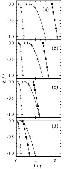
FIG. 2.: Phase diagram of binding energy $E$ vs. coupling constant $J$ for the extended $t$-$J$ model in the dilute limit for (a) $t^{\prime}=0.00~{}t$, (b) $t^{\prime}=-0.15~{}t$, (c) $t^{\prime}=-0.30~{}t$ and (d) $t^{\prime}=-0.45~{}t$. The solid line plots correspond to calculations done without the three-site term ($J_{3}=0$), the dashed lines for those done with the three-site term ($J_{3}=J$), the plots with open diamonds are for $s_{x^{2}+y^{2}}$-wave, and the plots with closed squares are for $d_{x^{2}-y^{2}}$-wave. The addition of the $J_{3}$-term causes the $s$-wave curves to shift left, whereas the $d$-wave curves shift right off to infinity; that is, there is no $d$-wave solution. The addition of the $t^{\prime}$-term causes $d$-wave (for $J_{3}=0$) to shift left and cross the $s$-wave curve at a point dependent upon the strength of $t^{\prime}$.

A phase diagram of $E$ vs. $J$ depicting the $s$- and $d$-wave bound states may be seen in Fig. 2(a). It can be noted from this low density phase diagram that $s$-wave always has the lower energy of the two solutions at fixed $J$ and is, therefore, the ground state of the problem at hand. Furthermore, $s$-wave has a bound state above a critical-$J$ ($J_{c}$) of $2.00~{}t$ whereas $d$-wave has a $J_{c}$ of about $7.32~{}t$. The phase diagram of Fig. 2(a) is identical to that reported recently by Hellberg and Manousakis [33] and the $s$-wave results are also similar to those of Kagan and Rice [34].

If one holds to the idea that magnetic pairing should produce $d$-wave, because of the hard core in the potential, the surprising aspect of these results is that $s$-wave always has by far the largest binding energy of the two symmetries. We may in fact prove a general theorem that if the potential has square symmetry, the ground state is always $s$-wave for nearest-neighbor hopping. This theorem holds whether there is a hard core or not. The proof is given first on the continuum with a radially symmetric potential, since it illustrates the main ideas most clearly. The Hamiltonian is

$${\cal H}=-\frac{\hbar^{2}}{2\mu}\left[\frac{1}{\rho}\frac{\partial}{\partial\rho}\left(\rho\frac{\partial}{\partial\rho}\right)+\frac{1}{\rho^{2}}\frac{\partial^{2}}{\partial\phi^{2}}\right]+V(\rho).$$ (78)

We argue by contradiction. Let $\psi_{m}(\rho,\phi)$ be the normalized ground state and have non-$s$-wave symmetry:

$$\psi_{m}(\rho,\phi)=\frac{1}{\sqrt{2\pi}}f(\rho)e^{im\phi},$$ (79)

with $m\neq 0$ and $\int_{0}^{\infty}\rho f^{2}(\rho)d\rho=1$. The ground state energy is

$$E_{m} = \left<\psi_{m}|{\cal H}|\psi_{m}\right>$$ (80)

$$= -\frac{\hbar^{2}}{2\mu}\int_{0}^{\infty}f(\rho)\frac{\partial}{\partial\rho}\left(\rho\frac{\partial f(\rho)}{\partial\rho}\right)d\rho$$ (83)

$$+\frac{m^{2}\hbar^{2}}{2\mu}\int_{0}^{\infty}\frac{1}{\rho}f^{2}(\rho)d\rho$$

$$+\int_{0}^{\infty}\rho f^{2}(\rho)V(\rho)d\rho.$$

Now consider the normalized trial wavefunction $\psi_{s}(\rho,\phi)=f(\rho)$, which is $s$-wave. This has the expectation value

$$E_{s} = \left<\psi_{s}|{\cal H}|\psi_{s}\right>$$ (84)

$$= -\frac{\hbar^{2}}{2\mu}\int_{0}^{\infty}f(\rho)\frac{\partial}{\partial\rho}\left(\rho\frac{\partial f(\rho)}{\partial\rho}\right)d\rho$$ (86)

$$+\int_{0}^{\infty}\rho f^{2}(\rho)V(\rho)d\rho.$$

Clearly,

$$E_{s}<E_{d}=E_{s}+\frac{m^{2}\hbar^{2}}{2\mu}\int_{0}^{\infty}\frac{1}{\rho}f^{2}(\rho)d\rho.$$ (87)

Thus $\psi_{m}$ cannot be the ground state. A similar proof obviously holds in three dimensions. The physics is simply that the increased kinetic energy from angular variations in a higher-wave wavefunction will always be greater than any gain in potential energy coming from avoidance of the core.

On the lattice, the physics is clearly the same, and the proof is quite similar. Let the potential $V({\bf r})$ have square symmetry, and let $t_{{\bf r},{\bf r^{\prime}}}$, the hopping coefficients, be positive. Let the assumed ground state be $\psi_{d}({\bf r})$ have $d$-wave ($B_{1}$) symmetry. It may be taken to be real. Now consider the wavefunction

$$\psi_{s}({\bf r})=|\psi_{d}({\bf r})|.$$ (88)

The expectation values are:

$$E_{d} = \left<\psi_{d}|{\cal H}|\psi_{d}\right>$$ (89)

$$= \sum_{\bf r}V({\bf r})\psi_{d}({\bf r})^{2}-\sum_{{\bf r}\neq{\bf r^{\prime}}}t_{{\bf r},{\bf r^{\prime}}}\psi_{d}({\bf r})\psi_{d}({\bf r^{\prime}}),$$ (90)

and

$$E_{s} = \left<\psi_{s}|{\cal H}|\psi_{s}\right>$$ (91)

$$= \sum_{\bf r}V({\bf r})\psi_{d}({\bf r})^{2}-\sum_{{\bf r}\neq{\bf r^{\prime}}}t_{{\bf r},{\bf r^{\prime}}}|\psi_{d}({\bf r})\psi_{d}({\bf r^{\prime}})|.$$ (92)

Comparison shows that

$$E_{s}\leq E_{d},$$ (93)

so that $\psi_{d}$ can never be the nondegenerate ground state. Except for pathological cases, it is not hard to improve $\psi_{s}$ to get a strict inequality in Eq. 93. (Let $\psi_{s}(x,x)\rightarrow\psi_{s}(x,x)+\delta\psi$, with $\delta$ sufficiently small). We have therefore shown that $s$-wave is in fact always the lowest energy solution. Hard core or not, $d$-wave never wins.

B The addition of the three-site terms

We now include the so-called three-site terms of the $t$-$J$ model in our dilute limit investigations. These added terms originate from the derivation of the $t$-$J$ model from the Hubbard model. Considering the Hubbard model,

$${\cal H}_{\text{Hubbard}}=-t\sum_{{\bf r},\mathchoice{{\hbox{\boldmath$\displaystyle\delta$}}}{{\hbox{\boldmath$\textstyle\delta$}}}{{\hbox{\boldmath$\scriptstyle\delta$}}}{{\hbox{\boldmath$\scriptscriptstyle\delta$}}},\sigma}c_{{\bf r},\sigma}^{\dagger}c_{{\bf r}+\mathchoice{{\hbox{\boldmath$\displaystyle\delta$}}}{{\hbox{\boldmath$\textstyle\delta$}}}{{\hbox{\boldmath$\scriptstyle\delta$}}}{{\hbox{\boldmath$\scriptscriptstyle\delta$}}},\sigma}+U\sum_{\bf r}n_{{\bf r}\uparrow}n_{{\bf r}\downarrow},$$ (94)

the $t$-term is treated as a perturbation with respect to the $U$-term, where $U\gg t$. Only terms up to and including order $t^{2}/U$ are retained. Letting $J\equiv 4t^{2}/U$, the perturbative expansion yields the $t$-$J$ Hamiltonian of Eq. (46) plus the three site terms [29]. The Hamiltonian may now be written

$${\cal H}_{tJJ_{3}} = -t\sum_{{\bf r},\mathchoice{{\hbox{\boldmath$\displaystyle\delta$}}}{{\hbox{\boldmath$\textstyle\delta$}}}{{\hbox{\boldmath$\scriptstyle\delta$}}}{{\hbox{\boldmath$\scriptscriptstyle\delta$}}},\sigma}c_{{\bf r},\sigma}^{\dagger}c_{{\bf r}+\mathchoice{{\hbox{\boldmath$\displaystyle\delta$}}}{{\hbox{\boldmath$\textstyle\delta$}}}{{\hbox{\boldmath$\scriptstyle\delta$}}}{{\hbox{\boldmath$\scriptscriptstyle\delta$}}},\sigma}$$ (98)

$$-\frac{J}{4}\sum_{{\bf r},\mathchoice{{\hbox{\boldmath$\displaystyle\delta$}}}{{\hbox{\boldmath$\textstyle\delta$}}}{{\hbox{\boldmath$\scriptstyle\delta$}}}{{\hbox{\boldmath$\scriptscriptstyle\delta$}}},\sigma}(n_{{\bf r},-\sigma}n_{{\bf r}+\mathchoice{{\hbox{\boldmath$\displaystyle\delta$}}}{{\hbox{\boldmath$\textstyle\delta$}}}{{\hbox{\boldmath$\scriptstyle\delta$}}}{{\hbox{\boldmath$\scriptscriptstyle\delta$}}},\sigma}+c_{{\bf r}+\mathchoice{{\hbox{\boldmath$\displaystyle\delta$}}}{{\hbox{\boldmath$\textstyle\delta$}}}{{\hbox{\boldmath$\scriptstyle\delta$}}}{{\hbox{\boldmath$\scriptscriptstyle\delta$}}},\sigma}^{\dagger}c_{{\bf r},-\sigma}^{\dagger}c_{{\bf r}+\mathchoice{{\hbox{\boldmath$\displaystyle\delta$}}}{{\hbox{\boldmath$\textstyle\delta$}}}{{\hbox{\boldmath$\scriptstyle\delta$}}}{{\hbox{\boldmath$\scriptscriptstyle\delta$}}},-\sigma}c_{{\bf r},\sigma})$$

$$-\frac{J_{3}}{4}\sum_{{\bf r},\mathchoice{{\hbox{\boldmath$\displaystyle\delta^{\prime}$}}}{{\hbox{\boldmath$\textstyle\delta^{\prime}$}}}{{\hbox{\boldmath$\scriptstyle\delta^{\prime}$}}}{{\hbox{\boldmath$\scriptscriptstyle\delta^{\prime}$}}}\neq\mathchoice{{\hbox{\boldmath$\displaystyle\delta$}}}{{\hbox{\boldmath$\textstyle\delta$}}}{{\hbox{\boldmath$\scriptstyle\delta$}}}{{\hbox{\boldmath$\scriptscriptstyle\delta$}}},\sigma}(c_{{\bf r}+\mathchoice{{\hbox{\boldmath$\displaystyle\delta$}}}{{\hbox{\boldmath$\textstyle\delta$}}}{{\hbox{\boldmath$\scriptstyle\delta$}}}{{\hbox{\boldmath$\scriptscriptstyle\delta$}}},\sigma}^{\dagger}n_{{\bf r},-\sigma}c_{{\bf r}+\mathchoice{{\hbox{\boldmath$\displaystyle\delta^{\prime}$}}}{{\hbox{\boldmath$\textstyle\delta^{\prime}$}}}{{\hbox{\boldmath$\scriptstyle\delta^{\prime}$}}}{{\hbox{\boldmath$\scriptscriptstyle\delta^{\prime}$}}},\sigma}$$

$$~{}~{}~{}~{}~{}~{}~{}~{}~{}~{}~{}~{}~{}~{}+c_{{\bf r}+\mathchoice{{\hbox{\boldmath$\displaystyle\delta$}}}{{\hbox{\boldmath$\textstyle\delta$}}}{{\hbox{\boldmath$\scriptstyle\delta$}}}{{\hbox{\boldmath$\scriptscriptstyle\delta$}}},\sigma}^{\dagger}c_{{\bf r},-\sigma}^{\dagger}c_{{\bf r}+\mathchoice{{\hbox{\boldmath$\displaystyle\delta^{\prime}$}}}{{\hbox{\boldmath$\textstyle\delta^{\prime}$}}}{{\hbox{\boldmath$\scriptstyle\delta^{\prime}$}}}{{\hbox{\boldmath$\scriptscriptstyle\delta^{\prime}$}}},-\sigma}c_{{\bf r},\sigma}),$$

where $J_{3}$ is merely used as an adjustable factor; letting $J_{3}=0$ restores Eq. (46), whereas letting $J_{3}=J$ yields the extended model as derived from the Hubbard model.

The three-site terms are usually dropped due to their complexity and the fact that their expectation value is formally of order $\delta J$, not $J$, where $\delta$ is the hole density. However, they are enhanced by the fact they are of order $z^{2}$, not $z$, where $z$ is the coordination number. Numerical results show clearly that they become important when $\delta$ is greater than $0.05$ [18]. Certainly, it would then be expected in the dilute limit that the three-site terms become very important interactions concerning the ground state energy of the system, and the solution to the extended model in the two-spin limit bears this out.

The solution of two spins interacting on a two-dimensional square lattice of $N_{s}$ sites is identical to that of Sec. IV A and need not be repeated here as now applied to Eq. (98). The wavefunction coefficients $a({\bf r})$ of Eq. (47) are found to have the following solutions (upon letting $N_{s}\rightarrow\infty$)

$$a_{s}({\bf r}) = J\left(1+\frac{3J_{3}}{J}\right)a(\mathchoice{{\hbox{\boldmath$\displaystyle\delta$}}}{{\hbox{\boldmath$\textstyle\delta$}}}{{\hbox{\boldmath$\scriptstyle\delta$}}}{{\hbox{\boldmath$\scriptscriptstyle\delta$}}}_{1})\frac{1}{(2\pi)^{2}}\int d{\bf k}e^{i{\bf k}\cdot{\bf r}}$$ (100)

$$\times\frac{\left(\cos{k_{x}}+\cos{k_{y}}-2I_{1}/I_{0}\right)}{\varepsilon({\bf k})-E/2},$$

$$a_{d}({\bf r}) = J\left(1-\frac{J_{3}}{J}\right)a(\mathchoice{{\hbox{\boldmath$\displaystyle\delta$}}}{{\hbox{\boldmath$\textstyle\delta$}}}{{\hbox{\boldmath$\scriptstyle\delta$}}}{{\hbox{\boldmath$\scriptscriptstyle\delta$}}}_{1})\frac{1}{(2\pi)^{2}}\int d{\bf k}e^{i{\bf k}\cdot{\bf r}}$$ (102)

$$\times\frac{\left(\cos{k_{x}}-\cos{k_{y}}\right)}{\varepsilon({\bf k})-E/2},$$

where $I_{0}$ and $I_{1}$ are still defined as in Eqs. (72) and (73), respectively. As expected, when $J_{3}=0$, the solutions of the $t$-$J$ model without three-site terms, Eqs. (69) and (71), are retrieved.

Given that $J_{3}=J$, it can be seen that there is only a trivial $d$-wave solution, namely $a_{d}({\bf r})=0$ for all ${\bf r}$. In other words, there is no bound state solution for $d$-wave pairing. The $s$-wave solution is similar to that of Eq. (69), differing only in pre-factors. Finding the relationship between $J$ and $E$ for these two solutions yields

$$\frac{1}{J_{s}} = \left(1+\frac{3J_{3}}{J}\right)\frac{1}{(2\pi)^{2}}\int d{\bf k}\cos{k_{x}}$$ (104)

$$\times\frac{\left(\cos{k_{x}}+\cos{k_{y}}-2I_{1}/I_{0}\right)}{\varepsilon({\bf k})-E/2},$$

$$\frac{1}{J_{d}} = \left(1-\frac{J_{3}}{J}\right)\frac{1}{(2\pi)^{2}}\int d{\bf k}\cos{k_{x}}$$ (106)

$$\times\frac{\left(\cos{k_{x}}-\cos{k_{y}}\right)}{\varepsilon({\bf k})-E/2}.$$

It can be readily seen that, as the three-site interactions are “turned on”, that is as $J_{3}$ is increased from $0$ to $J$, the $J$ vs. $E$ curve for $d$-wave would move off to infinity in the phase diagram of Fig. 2(a). This again shows that there is no bound state solution for $d$-wave in the dilute limit of the extended $t$-$J$ model. For $s$-wave, the $J$ vs. $E$ curve is exactly one fourth that of the $s$-wave solution for the “traditional” $t$-$J$ model as shown in Fig. 2(a). Thus, the three-site terms are $s$-wave enhancing, $d$-wave suppressing interactions.

The expectation values of the various terms of the extended $t$-$J$ model can be expressed in terms of the wavefunction coefficients $a({\bf r})$ as well as in integral forms. The normalization is

$$\left<\psi|\psi\right> = \sum_{{\bf r}_{1},{\bf r}_{2}}|a({\bf r}_{1}-{\bf r}_{2})|^{2}$$ (107)

$$= J^{2}B_{J_{3}}^{2}|a(\mathchoice{{\hbox{\boldmath$\displaystyle\delta$}}}{{\hbox{\boldmath$\textstyle\delta$}}}{{\hbox{\boldmath$\scriptstyle\delta$}}}{{\hbox{\boldmath$\scriptscriptstyle\delta$}}}_{1})|^{2}\frac{N_{s}}{(2\pi)^{2}}\int d{\bf k}A_{k}^{2},$$ (108)

where $N_{s}$ is temporarily left finite but will cancel out in the expectation values shown below. The coefficients $B_{J_{3}}$ and $A_{\bf k}$ are defined for convenience as

$$A_{\bf k} = (\cos{k_{x}}+\cos{k_{y}}-2I_{1}/I_{0})/(\varepsilon({\bf k})-E/2),$$ (109)

$$B_{J_{3}} = 1+3J_{3}/J$$ (110)

for $s$-wave and

$$A_{\bf k} = (\cos{k_{x}}-\cos{k_{y}})/(\varepsilon({\bf k})-E/2),$$ (111)

$$B_{J_{3}} = 1-J_{3}/J$$ (112)

for $d$-wave.

The expectation values can now be expressed in terms of integrals. The relations between $J$ and $E$ from Eqs. (104) and (106) are also employed to yield

$$\left<{\cal H}_{t}\right> = \frac{\left<\psi|{\cal H}_{t}|\psi\right>}{\left<\psi|\psi\right>}$$ (113)

$$= -4t\frac{\int d{\bf k}A_{\bf k}^{2}(\cos{k_{x}}+\cos{k_{y}})}{\int d{\bf k}A_{\bf k}^{2}},$$ (114)

$$\left<{\cal H}_{J}\right> = \frac{\left<\psi|{\cal H}_{J}|\psi\right>}{\left<\psi|\psi\right>}$$ (115)

$$= -\frac{4}{B_{J_{3}}}\frac{\int d{\bf k}A_{\bf k}\cos{k_{x}}}{\int d{\bf k}A_{\bf k}^{2}},$$ (116)

$$\left<{\cal H}_{J_{3}}\right> = \frac{\left<\psi|{\cal H}_{J_{3}}|\psi\right>}{\left<\psi|\psi\right>}$$ (117)

$$= -\frac{12}{B_{J_{3}}}\left(\frac{J_{3}}{J}\right)\frac{\int d{\bf k}A_{\bf k}\cos{k_{x}}}{\int d{\bf k}A_{\bf k}^{2}},\hskip 7.22743pt\text{$s$-wave}$$ (118)

$$= +\frac{4}{B_{J_{3}}}\left(\frac{J_{3}}{J}\right)\frac{\int d{\bf k}A_{\bf k}\cos{k_{x}}}{\int d{\bf k}A_{\bf k}^{2}},\hskip 7.22743pt\text{$d$-wave}.$$ (119)

Of course, the solutions for $d$-wave are ill-defined for $J_{3}=J$ ($a_{d}({\bf k})=0$ for all ${\bf k}$ in this case) but are included here merely for completeness. What can be immediately seen is that, for $s$-wave, the three-site term has an expectation value exactly three times that of the $J$-term, or $\left<{\cal H}_{J_{3}}\right>=3\left<{\cal H}_{J}\right>$, and for $d$-wave, the two expectation values are equal and opposite, or $\left<{\cal H}_{J_{3}}\right>=-\left<{\cal H}_{J}\right>$.

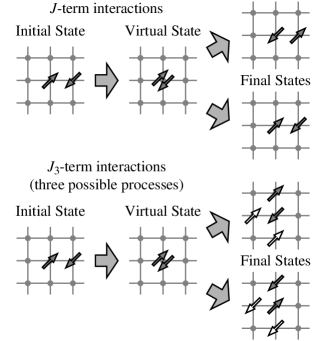
FIG. 3.: Diagram of the dynamics of the spin-spin correlation term (or $J$-term) and the three-site term (or $J_{3}$-term). Shown are initial, intermediate (or virtual), and final states for one example of each interaction (filled arrows). For the $J_{3}$-term, alternative interactions are also shown (open arrows). In these examples, a down spin has a virtual hopping to a nearest-neighbor site occupied by an up spin. In the $J$-term, either spin hops back to the original site, and in the $J_{3}$-term, either spin hops to one of the other three nearest-neighbor sites. In the dilute limit, the spins have equal probability of hopping to any of the four nearest-neighbor sites as shown here. In the Cooper problem, however, there would be a probability of $\delta$ for each of the three originally unoccupied nearest-neighbor sites to actually be occupied by a non-interacting spin.

A closer look at the various interactions of the extended $t$-$J$ model in the dilute limit is worth making at this point. It is obvious from the Hamiltonian as written in Eq. (98) that the $J_{3}$-term is quite similar to the $J$-term. The three-site terms comprise interactions involving a site and two distinct nearest-neighbors, whereas the $J$-term is the special case where the two nearest-neighbor sites are merely the same site. Figure 3 shows a depiction of the virtual processes involved in the spin-spin correlation term ($J$-term) and the three-site terms ($J_{3}$-term). When the two spins are on nearest-neighbor sites, the $J$-term can be thought of as a virtual hopping of one spin onto the site occupied by the other spin, followed by either spin hopping back to the first site. In the dilute limit, the probability of finding the other three nearest-neighbor sites unoccupied is exactly $1$. Hence, when one spin has a virtual hopping onto the site occupied by the other spin, there is equal chance of one of the spins hopping onto any of the four nearest-neighbors. For $s$-wave, it is easy to see then why the $J_{3}$-term is three times the size of the $J$-term, and, due to its change of sign with $\pi/2$ rotation, the $d$-wave $J_{3}$-term is equal to the $J$-term but with opposite sign. Hence, the total summation of the $J_{3}$- and $J$-terms for $d$-wave yields zero due to its symmetry, and the total summation for $s$-wave yields four times the value of the $J$-term. The importance of this result will become more apparent in Sec. V where increasing spin density is considered in the Cooper problem. The actual effect of the three-site terms is more akin to a kinetic energy term than an interaction term. It is an effective hopping to second- and third-nearest-neighbors. It is therefore not so surprising that it tends to stabilize the $s$-wave state.

C The addition of the next-nearest-neighbor hopping term

One more interaction is included in our extended $t$-$J$ model, namely the next-nearest-neighbor hopping term. This term is added with the intent of making a first approximation at modeling specific high-temperature superconducting systems. It is known, for example from neutron scattering, that the various high-$T_{c}$ copper-oxides differ in energy dispersion, Fermi surface, etc. Using the next-nearest-neighbor hopping term with coefficient $t^{\prime}$ is a way of distinguishing these compounds from one another in our tight-binding model. Perhaps a more systematic approach, emulating our derivation of the $J_{3}$-term, would be to begin with the Hubbard model and include the $t^{\prime}$-term in the large-$U$ perturbative expansion. This would result in more terms of order $J$, that is various three-site terms involving nearest-neighbor sites, next-nearest-neighbor sites, and mixtures of both. The many extra terms may be worth studying at some future time, but for the purposes of identifying trends in the $t$-$J$ model, we do not wish to introduce even more complexity to our extended model until it has been sufficiently investigated in its present form.

The extended $t$-$J$ model is given in its full form as

$${\cal H}_{tt^{\prime}JJ_{3}} = -t\sum_{{\bf r},\mathchoice{{\hbox{\boldmath$\displaystyle\delta$}}}{{\hbox{\boldmath$\textstyle\delta$}}}{{\hbox{\boldmath$\scriptstyle\delta$}}}{{\hbox{\boldmath$\scriptscriptstyle\delta$}}},\sigma}c_{{\bf r},\sigma}^{\dagger}c_{{\bf r}+\mathchoice{{\hbox{\boldmath$\displaystyle\delta$}}}{{\hbox{\boldmath$\textstyle\delta$}}}{{\hbox{\boldmath$\scriptstyle\delta$}}}{{\hbox{\boldmath$\scriptscriptstyle\delta$}}},\sigma}-t^{\prime}\sum_{{\bf r},\mathchoice{{\hbox{\boldmath$\displaystyle\gamma$}}}{{\hbox{\boldmath$\textstyle\gamma$}}}{{\hbox{\boldmath$\scriptstyle\gamma$}}}{{\hbox{\boldmath$\scriptscriptstyle\gamma$}}},\sigma}c_{{\bf r},\sigma}^{\dagger}c_{{\bf r}+\mathchoice{{\hbox{\boldmath$\displaystyle\gamma$}}}{{\hbox{\boldmath$\textstyle\gamma$}}}{{\hbox{\boldmath$\scriptstyle\gamma$}}}{{\hbox{\boldmath$\scriptscriptstyle\gamma$}}},\sigma}$$ (124)

$$-\frac{J}{4}\sum_{{\bf r},\mathchoice{{\hbox{\boldmath$\displaystyle\delta$}}}{{\hbox{\boldmath$\textstyle\delta$}}}{{\hbox{\boldmath$\scriptstyle\delta$}}}{{\hbox{\boldmath$\scriptscriptstyle\delta$}}},\sigma}(n_{{\bf r},-\sigma}n_{{\bf r}+\mathchoice{{\hbox{\boldmath$\displaystyle\delta$}}}{{\hbox{\boldmath$\textstyle\delta$}}}{{\hbox{\boldmath$\scriptstyle\delta$}}}{{\hbox{\boldmath$\scriptscriptstyle\delta$}}},\sigma}$$

$$~{}~{}~{}~{}~{}~{}~{}~{}~{}+c_{{\bf r}+\mathchoice{{\hbox{\boldmath$\displaystyle\delta$}}}{{\hbox{\boldmath$\textstyle\delta$}}}{{\hbox{\boldmath$\scriptstyle\delta$}}}{{\hbox{\boldmath$\scriptscriptstyle\delta$}}},\sigma}^{\dagger}c_{{\bf r},-\sigma}^{\dagger}c_{{\bf r}+\mathchoice{{\hbox{\boldmath$\displaystyle\delta$}}}{{\hbox{\boldmath$\textstyle\delta$}}}{{\hbox{\boldmath$\scriptstyle\delta$}}}{{\hbox{\boldmath$\scriptscriptstyle\delta$}}},-\sigma}c_{{\bf r},\sigma})$$

$$-\frac{J_{3}}{4}\sum_{{\bf r},\mathchoice{{\hbox{\boldmath$\displaystyle\delta^{\prime}$}}}{{\hbox{\boldmath$\textstyle\delta^{\prime}$}}}{{\hbox{\boldmath$\scriptstyle\delta^{\prime}$}}}{{\hbox{\boldmath$\scriptscriptstyle\delta^{\prime}$}}}\neq\mathchoice{{\hbox{\boldmath$\displaystyle\delta$}}}{{\hbox{\boldmath$\textstyle\delta$}}}{{\hbox{\boldmath$\scriptstyle\delta$}}}{{\hbox{\boldmath$\scriptscriptstyle\delta$}}},\sigma}(c_{{\bf r}+\mathchoice{{\hbox{\boldmath$\displaystyle\delta$}}}{{\hbox{\boldmath$\textstyle\delta$}}}{{\hbox{\boldmath$\scriptstyle\delta$}}}{{\hbox{\boldmath$\scriptscriptstyle\delta$}}},\sigma}^{\dagger}n_{{\bf r},-\sigma}c_{{\bf r}+\mathchoice{{\hbox{\boldmath$\displaystyle\delta^{\prime}$}}}{{\hbox{\boldmath$\textstyle\delta^{\prime}$}}}{{\hbox{\boldmath$\scriptstyle\delta^{\prime}$}}}{{\hbox{\boldmath$\scriptscriptstyle\delta^{\prime}$}}},\sigma}$$

$$~{}~{}~{}~{}~{}~{}~{}~{}~{}~{}~{}~{}~{}~{}+c_{{\bf r}+\mathchoice{{\hbox{\boldmath$\displaystyle\delta$}}}{{\hbox{\boldmath$\textstyle\delta$}}}{{\hbox{\boldmath$\scriptstyle\delta$}}}{{\hbox{\boldmath$\scriptscriptstyle\delta$}}},\sigma}^{\dagger}c_{{\bf r},-\sigma}^{\dagger}c_{{\bf r}+\mathchoice{{\hbox{\boldmath$\displaystyle\delta^{\prime}$}}}{{\hbox{\boldmath$\textstyle\delta^{\prime}$}}}{{\hbox{\boldmath$\scriptstyle\delta^{\prime}$}}}{{\hbox{\boldmath$\scriptscriptstyle\delta^{\prime}$}}},-\sigma}c_{{\bf r},\sigma}),$$

where summation over $\textstyle\gamma$ means summation over next-nearest-neighbor sites. Once again considering the problem in the dilute limit, the solution to the problem of two spins interacting with the Hamiltonian of Eq. (124) results in exactly the same forms for $a_{s}({\bf r})$ and $a_{d}({\bf r})$ as given in Eqs. (100) and (102), respectively, only now, the tight-binding energy dispersion is given by $\varepsilon({\bf k})=-2t(\cos{k_{x}}+\cos{k_{y}})-4t^{\prime}\cos{k_{x}}\cos{k_{y}}$.

The relationships between $J$ and $E$ are of the same forms as given in Eqs. (104) and (106) for $s$-wave and $d$-wave, respectively. Once again, phase diagrams for $E$ vs. $J$ can be drawn for various values of $t^{\prime}$. Fig. 2(a) is, obviously, the phase diagram with $t^{\prime}=0$. Figs. 2(b), (c), and (d) show the phase diagrams for $t^{\prime}=-0.15~{}t$, $-0.30~{}t$, and $-0.45~{}t$, respectively. It can be seen that, for finite $t^{\prime}$ and no three-site interactions, the $s$-wave and $d$-wave curves cross at a binding energy $E$ and value $J$ which decrease with increasing magnitude of $t^{\prime}$. In other words, as the next-nearest-neighbor hopping term increases in strength, there is a cross-over between an $s$-wave ground state solution and a $d$-wave ground state solution at smaller and smaller binding energies and $J$-values. This shows that the $t^{\prime}$-term with a negative sign is an $s$-wave suppressing, $d$-wave enhancing term in the model. That this must be the case is evident already from Eqs. (90) and (92). Once again, when the three-site terms are considered ($J_{3}=J$), there is no $d$-wave solution in the dilute limit, and the $s$-wave curve is reduced to a quarter of its value without the $J_{3}$-term.

The physics of the dilute limit is that, in the absence of a Fermi surface, the $s$-wave instability is dominant. The $s$-wave simply has lower kinetic energy. In the next section we present an investigation of a single pair now interacting in the presence of a Fermi surface: the extended $t$-$J$ model is evaluated in the Cooper problem.

V The Cooper Problem

The investigations of Sec. IV can now be extended from the dilute limit to the regime of finite density. Again, the purpose of this study is to identify trends with the addition of the three-site term, with the changing of the next-nearest-neighbor hopping term, and now with the changing of the density of spins. As before, the problem is solved for one pair of interacting spins, now being in the presence of a filled Fermi sea of non-interacting spins. These results will be compared qualitatively with previous VMC results which also yield some of the trends detailed in this work.

Consider the problem again of two spins interacting on a square, two-dimensional lattice of $N_{s}$ sites, but now allow them to interact in the presence of a filled Fermi sea up to a Fermi energy (chemical potential) of $\mu$. This is the Cooper problem as applied to the extended $t$-$J$ model. As we shall show, this also corresponds again to the stability form of the gap equation at zero temperature with a certain interaction.

The solution once again entails finding the wavefunction coefficients $a({\bf r})$ Eq. (47) from the Schrödinger equation Eq. (44) which is now rewritten

$$\tilde{\cal H}_{tt^{\prime}JJ_{3}}\left|\psi\right>=(2\mu+E)\left|\psi\right>,$$ (125)

where the eigenvalue $E$ has been redefined with respect to the Fermi energy. Once again, $\tilde{\cal H}_{tt^{\prime}JJ_{3}}$ must include an on-site repulsion term so that the solution will enforce no-double-occupancy as was shown in Eq. (49). In a similar fashion, the states within the Fermi surface must be excluded from any interactions since they are to be filled with non-interacting spins. This is still a two-particle problem which reduces to a single-particle equation as in Eq. (51), but with a fictitious interaction coming from the Pauli exclusion principle. The exclusion of states within the Fermi surface is taken into account by adding another term to $\tilde{\cal H}_{tt^{\prime}JJ_{3}}$, namely

$$\tilde{\cal H}_{tt^{\prime}JJ_{3}}\rightarrow\tilde{\cal H}_{tt^{\prime}JJ_{3}}+\sum_{{\bf k},\sigma}U_{C}({\bf k})n_{{\bf k},\sigma}$$ (126)

with the following dependence on ${\bf k}$:

$$U_{C}({\bf k})=\left\{\begin{array}[]{ll}U_{C}^{0},&\xi({\bf k})<0\\ 0,&\xi({\bf k})>0\end{array}\right.,$$ (127)

where $\xi({\bf k})=\varepsilon({\bf k})-\mu$. Thus, the same technique as with the exclusion of doubly-occupied sites can be employed: the limit of $U_{C}^{0}\rightarrow\infty$ at the end of the derivation will exclude states within the Fermi surface.

An important observation needs to be made concerning the three-site terms. Figure 3 shows the dynamics of the $J$-term and $J_{3}$-term in the dilute limit, where the $J_{3}$-term has three times the value of the $J$-term for extended $s$-wave and the same value and opposite sign for $d$-wave. This is due to the fact that, if the two spins occupy nearest-neighbor sites, the other three nearest-neighbor sites would then be guaranteed unoccupied in the dilute limit. Now, however, with finite density, if the two interacting spins are on nearest-neighbor sites, then there would be a virtual hopping onto one of the sites, and the probability of the original nearest-neighbor being unoccupied would be $1$, whereas the probability of the other three nearest-neighbors being unoccupied would be $\delta$, the hole density. In other words, the three-site terms need to have a pre-factor of $\delta$ to take into account the finite density of non-interacting spins now present on the lattice. In addition to this, the nearest-neighbor and next-nearest-neighbor hopping terms must also both have pre-factors of $\delta$ to reflect this finite probability that a site to which one of the two interacting spins may hop could be occupied by one of the non-interacting spins. Given all of these necessary changes, the Hamiltonian (without the additional $V_{0}$- and $U_{C}$-potential terms) should now be expressed as

$${\cal H}_{tt^{\prime}JJ_{3}} = -\delta t\sum_{{\bf r},\mathchoice{{\hbox{\boldmath$\displaystyle\delta$}}}{{\hbox{\boldmath$\textstyle\delta$}}}{{\hbox{\boldmath$\scriptstyle\delta$}}}{{\hbox{\boldmath$\scriptscriptstyle\delta$}}},\sigma}c_{{\bf r},\sigma}^{\dagger}c_{{\bf r}+\mathchoice{{\hbox{\boldmath$\displaystyle\delta$}}}{{\hbox{\boldmath$\textstyle\delta$}}}{{\hbox{\boldmath$\scriptstyle\delta$}}}{{\hbox{\boldmath$\scriptscriptstyle\delta$}}},\sigma}-\delta t^{\prime}\sum_{{\bf r},\mathchoice{{\hbox{\boldmath$\displaystyle\gamma$}}}{{\hbox{\boldmath$\textstyle\gamma$}}}{{\hbox{\boldmath$\scriptstyle\gamma$}}}{{\hbox{\boldmath$\scriptscriptstyle\gamma$}}},\sigma}c_{{\bf r},\sigma}^{\dagger}c_{{\bf r}+\mathchoice{{\hbox{\boldmath$\displaystyle\gamma$}}}{{\hbox{\boldmath$\textstyle\gamma$}}}{{\hbox{\boldmath$\scriptstyle\gamma$}}}{{\hbox{\boldmath$\scriptscriptstyle\gamma$}}},\sigma}$$ (132)

$$-\frac{J}{4}\sum_{{\bf r},\mathchoice{{\hbox{\boldmath$\displaystyle\delta$}}}{{\hbox{\boldmath$\textstyle\delta$}}}{{\hbox{\boldmath$\scriptstyle\delta$}}}{{\hbox{\boldmath$\scriptscriptstyle\delta$}}},\sigma}(n_{{\bf r},-\sigma}n_{{\bf r}+\mathchoice{{\hbox{\boldmath$\displaystyle\delta$}}}{{\hbox{\boldmath$\textstyle\delta$}}}{{\hbox{\boldmath$\scriptstyle\delta$}}}{{\hbox{\boldmath$\scriptscriptstyle\delta$}}},\sigma}$$

$$~{}~{}~{}~{}~{}~{}~{}~{}~{}~{}+c_{{\bf r}+\mathchoice{{\hbox{\boldmath$\displaystyle\delta$}}}{{\hbox{\boldmath$\textstyle\delta$}}}{{\hbox{\boldmath$\scriptstyle\delta$}}}{{\hbox{\boldmath$\scriptscriptstyle\delta$}}},\sigma}^{\dagger}c_{{\bf r},-\sigma}^{\dagger}c_{{\bf r}+\mathchoice{{\hbox{\boldmath$\displaystyle\delta$}}}{{\hbox{\boldmath$\textstyle\delta$}}}{{\hbox{\boldmath$\scriptstyle\delta$}}}{{\hbox{\boldmath$\scriptscriptstyle\delta$}}},-\sigma}c_{{\bf r},\sigma})$$

$$-\delta\frac{J_{3}}{4}\sum_{{\bf r},\mathchoice{{\hbox{\boldmath$\displaystyle\delta^{\prime}$}}}{{\hbox{\boldmath$\textstyle\delta^{\prime}$}}}{{\hbox{\boldmath$\scriptstyle\delta^{\prime}$}}}{{\hbox{\boldmath$\scriptscriptstyle\delta^{\prime}$}}}\neq\mathchoice{{\hbox{\boldmath$\displaystyle\delta$}}}{{\hbox{\boldmath$\textstyle\delta$}}}{{\hbox{\boldmath$\scriptstyle\delta$}}}{{\hbox{\boldmath$\scriptscriptstyle\delta$}}},\sigma}(c_{{\bf r}+\mathchoice{{\hbox{\boldmath$\displaystyle\delta$}}}{{\hbox{\boldmath$\textstyle\delta$}}}{{\hbox{\boldmath$\scriptstyle\delta$}}}{{\hbox{\boldmath$\scriptscriptstyle\delta$}}},\sigma}^{\dagger}n_{{\bf r},-\sigma}c_{{\bf r}+\mathchoice{{\hbox{\boldmath$\displaystyle\delta^{\prime}$}}}{{\hbox{\boldmath$\textstyle\delta^{\prime}$}}}{{\hbox{\boldmath$\scriptstyle\delta^{\prime}$}}}{{\hbox{\boldmath$\scriptscriptstyle\delta^{\prime}$}}},\sigma}$$

$$~{}~{}~{}~{}~{}~{}~{}~{}~{}~{}~{}~{}~{}~{}~{}~{}+c_{{\bf r}+\mathchoice{{\hbox{\boldmath$\displaystyle\delta$}}}{{\hbox{\boldmath$\textstyle\delta$}}}{{\hbox{\boldmath$\scriptstyle\delta$}}}{{\hbox{\boldmath$\scriptscriptstyle\delta$}}},\sigma}^{\dagger}c_{{\bf r},-\sigma}^{\dagger}c_{{\bf r}+\mathchoice{{\hbox{\boldmath$\displaystyle\delta^{\prime}$}}}{{\hbox{\boldmath$\textstyle\delta^{\prime}$}}}{{\hbox{\boldmath$\scriptstyle\delta^{\prime}$}}}{{\hbox{\boldmath$\scriptscriptstyle\delta^{\prime}$}}},-\sigma}c_{{\bf r},\sigma}),$$

Upon solving for $a({\bf r})$ and self-consistently solving for $a(0)$ and the four $a(\delta)$’s, two solutions are again obtained of the forms

$$a_{s}({\bf r}) = J\left(1+3\delta\frac{J_{3}}{J}\right)a(\mathchoice{{\hbox{\boldmath$\displaystyle\delta$}}}{{\hbox{\boldmath$\textstyle\delta$}}}{{\hbox{\boldmath$\scriptstyle\delta$}}}{{\hbox{\boldmath$\scriptscriptstyle\delta$}}}_{1})\frac{1}{(2\pi)^{2}}\int d{\bf k}e^{i{\bf k}\cdot{\bf r}}$$ (134)

$$\times\frac{\left(\cos{k_{x}}+\cos{k_{y}}-2I_{1}/I_{0}\right)}{\delta\xi({\bf k})-E/2+U_{C}({\bf k})},$$

$$a_{d}({\bf r}) = J\left(1-\delta\frac{J_{3}}{J}\right)a(\mathchoice{{\hbox{\boldmath$\displaystyle\delta$}}}{{\hbox{\boldmath$\textstyle\delta$}}}{{\hbox{\boldmath$\scriptstyle\delta$}}}{{\hbox{\boldmath$\scriptscriptstyle\delta$}}}_{1})\frac{1}{(2\pi)^{2}}\int d{\bf k}e^{i{\bf k}\cdot{\bf r}}$$ (136)

$$\times\frac{\left(\cos{k_{x}}-\cos{k_{y}}\right)}{\delta\xi({\bf k})-E/2+U_{C}({\bf k})},$$

which once again correspond to extended $s$-wave and $d$-wave solutions, respectively.. Here, the limit $V_{0}\rightarrow\infty$ has already been done. Now the definition of $U_{C}({\bf k})$ from Eq. (127) can be used, and the limit of $U_{C}^{0}\rightarrow\infty$ is taken, yielding the final solutions

$$a_{s}({\bf r}) = J\left(1+3\delta\frac{J_{3}}{J}\right)a(\mathchoice{{\hbox{\boldmath$\displaystyle\delta$}}}{{\hbox{\boldmath$\textstyle\delta$}}}{{\hbox{\boldmath$\scriptstyle\delta$}}}{{\hbox{\boldmath$\scriptscriptstyle\delta$}}}_{1})\frac{1}{(2\pi)^{2}}\int_{\xi({\bf k})>0}d{\bf k}e^{i{\bf k}\cdot{\bf r}}$$ (138)

$$\times\frac{\left(\cos{k_{x}}+\cos{k_{y}}-2I_{1}/I_{0}\right)}{\delta\xi({\bf k})-E/2},$$

$$a_{d}({\bf r}) = J\left(1-\delta\frac{J_{3}}{J}\right)a(\mathchoice{{\hbox{\boldmath$\displaystyle\delta$}}}{{\hbox{\boldmath$\textstyle\delta$}}}{{\hbox{\boldmath$\scriptstyle\delta$}}}{{\hbox{\boldmath$\scriptscriptstyle\delta$}}}_{1})\frac{1}{(2\pi)^{2}}\int_{\xi({\bf k})>0}d{\bf k}e^{i{\bf k}\cdot{\bf r}}$$ (140)

$$\times\frac{\left(\cos{k_{x}}-\cos{k_{y}}\right)}{\delta\xi({\bf k})-E/2}.$$

Integrations are, therefore, done over those states lying outside of the Fermi surface; the filled states do not contribute to the interactions of the problem.

The relationship for $J$ and $E$ can be found for the finite density problem as well as the expectation values of the various terms of the extended $t$-$J$ Hamiltonian. The equations connecting $J$ and $E$ can be expressed as

$$\frac{1}{J}=B_{J_{3}}\frac{1}{(2\pi)^{2}}\int_{\xi({\bf k})>0}d{\bf k}\cos{k_{x}}A_{\bf k},$$ (141)

where now

$$A_{\bf k} = (\cos{k_{x}}+\cos{k_{y}}-2I_{1}/I_{0})/(\delta\xi({\bf k})-E/2),$$ (142)

$$B_{J_{3}} = 1+3\delta J_{3}/J$$ (143)

for $s$-wave and

$$A_{\bf k} = (\cos{k_{x}}-\cos{k_{y}})/(\delta\xi({\bf k})-E/2),$$ (144)

$$B_{J_{3}} = 1-\delta J_{3}/J$$ (145)

for $d$-wave. The integrals in Eq. (141) cannot be done analytically. The actual calculations entailed a simple Monte Carlo integration method where special care was taken when $E$ was small and the denominator of the integrand tended towards zero along the Fermi surface.

These eigenvalue-type equations can again be shown to be equivalent to the stability form of the gap equation at zero temperature. The difference with the dilute case is that the interaction $V_{\text{gap}}$ which appears in the gap equation now has a frequency cutoff

$$V_{\text{gap}}({\bf k},{\bf k^{\prime}})=\left\{\begin{array}[]{ll}V({\bf k},{\bf k^{\prime}}),&\xi({\bf k})>0\\ 0,&\xi({\bf k})<0.\end{array}\right.$$ (146)

This looks artificial. However, the Cooper bound state equation in the conventional case has the same asymmetrical cutoff. The difference between the asymmetrical cutoff and the more symmetrical cutoff of the BCS interaction is in fact responsible for the factor of two difference in the exponential factors in the Cooper binding energy and the BCS gap. Again, this difference does not influence the stability issue of interest here.

The normalization is found to be

$$\left<\psi|\psi\right> = \sum_{{\bf r}_{1},{\bf r}_{2}}|a({\bf r}_{1}-{\bf r}_{2})|^{2}$$ (147)

$$= J^{2}B_{J_{3}}^{2}|a(\mathchoice{{\hbox{\boldmath$\displaystyle\delta$}}}{{\hbox{\boldmath$\textstyle\delta$}}}{{\hbox{\boldmath$\scriptstyle\delta$}}}{{\hbox{\boldmath$\scriptscriptstyle\delta$}}}_{1})|^{2}\frac{N_{s}}{(2\pi)^{2}}\int_{\xi({\bf k})>0}d{\bf k}A_{k}^{2},$$ (148)

and the expectation values of the terms may be expressed

$$\left<{\cal H}_{t}\right> = \frac{\left<\psi|{\cal H}_{t}|\psi\right>}{\left<\psi|\psi\right>}$$ (149)

$$= -4\delta t\frac{\int_{\xi({\bf k})>0}d{\bf k}A_{\bf k}^{2}(\cos{k_{x}}+\cos{k_{y}})}{\int_{\xi({\bf k})>0}d{\bf k}A_{\bf k}^{2}},$$ (150)

$$\left<{\cal H}_{t^{\prime}}\right> = \frac{\left<\psi|{\cal H}_{t^{\prime}}|\psi\right>}{\left<\psi|\psi\right>}$$ (151)

$$= -8\delta t^{\prime}\frac{\int_{\xi({\bf k})>0}d{\bf k}A_{\bf k}^{2}\cos{k_{x}}\cos{k_{y}}}{\int_{\xi({\bf k})>0}d{\bf k}A_{\bf k}^{2}},$$ (152)

$$\left<{\cal H}_{J}\right> = \frac{\left<\psi|{\cal H}_{J}|\psi\right>}{\left<\psi|\psi\right>}$$ (153)

$$= -\frac{4}{B_{J_{3}}}\frac{\int_{\xi({\bf k})>0}d{\bf k}A_{\bf k}\cos{k_{x}}}{\int_{\xi({\bf k})>0}d{\bf k}A_{\bf k}^{2}},$$ (154)

$$\left<{\cal H}_{J_{3}}\right> = \frac{\left<\psi|{\cal H}_{J_{3}}|\psi\right>}{\left<\psi|\psi\right>}$$ (155)

$$= -\frac{12}{B_{J_{3}}}\left(\delta\frac{J_{3}}{J}\right)\frac{\int_{\xi({\bf k})>0}d{\bf k}A_{\bf k}\cos{k_{x}}}{\int_{\xi({\bf k})>0}d{\bf k}A_{\bf k}^{2}},\text{$s$},$$ (156)

$$= +\frac{4}{B_{J_{3}}}\left(\delta\frac{J_{3}}{J}\right)\frac{\int_{\xi({\bf k})>0}d{\bf k}A_{\bf k}\cos{k_{x}}}{\int_{\xi({\bf k})>0}d{\bf k}A_{\bf k}^{2}},\text{$d$}.$$ (157)

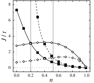
FIG. 4.: Phase diagram of coupling constant $J$ vs. spin density $n$ in the Cooper problem for binding energy $E=-0.01~{}t$, $J_{3}=0$ (solid line), and $J_{3}=J$ (dashed line). The cross-over points between $d$- (closed squares) and $s$-wave (open diamonds) occur at specific densities for both cases, where these densities remain fairly fixed as $E$ (and accordingly $J$) is decreased even more. With the addition of the three-site term, $s$-wave commands more of the phase diagram while $d$-wave is suppressed.

Equation (141) is divergent in the limit $E\rightarrow 0$. In other words, given the presence of a Fermi surface ($\delta<1$ and $n>0$), $J$ does not have a finite critical value as it did in the dilute limit ($\delta=1$ and $n=0$). This means that there exists a bound state ($E<0$) for any potential $J$ no matter how small. This is indeed the conclusion of the Cooper problem: any pairing potential has a bound state for one pair of spins, and this must extend to the case of multiple pairs of spins. It is now important to see which of the two symmetries has the largest binding energy $E$ (in absolute value) for a given $J$ as both $t^{\prime}$ and $\delta$ are varied. In reality, $J$ is expressed as an integral containing $E$, and so $E$ is fixed as $J$ is calculated for varying values of both $t^{\prime}$ and $\delta$. Fig. 4 shows the diagram of $J$ vs. $n$ for a fixed binding energy $E=-0.01~{}t$ for $t^{\prime}=0$ and $J_{3}=0$. The curves for $s$-wave and $d$-wave cross at a density of about $n=0.2$. This means that $d$-wave has the larger binding energy at smaller potential $J$ for densities $n>0.2$, whereas $s$-wave has the larger binding energy at smaller $J$ for $n<0.2$. Turning this statement around, given a set $J$, $d$-wave would have the higher binding energy for $n>0.2$ and $s$-wave would be dominant for $n<0.2$. Indeed, if the curves of $J$ vs. $n$ (as calculated from the above derivations) were to be plotted as in Fig. 4 for decreasing values of the binding energy ($E\rightarrow 0$), this cross-over point would remain relatively fixed even as the $J$-curves collapsed to $J=0$ over all $n$ at $E=0$. This cross-over between an $s$- and $d$-wave phase near $n=0.2$ has been seen by Dagotto, et al., in a quite different low-density study [35].

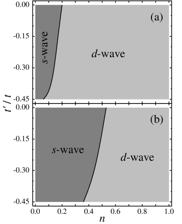
FIG. 5.: Phase diagram of next-nearest-neighbor hopping parameter $t^{\prime}$ vs. spin density $n$ in the Cooper problem for (a) $J_{3}=0$ and (b) $J_{3}=J$. The phase boundary represents small binding energy $E$ (and, therefore, small coupling constant $J$). These diagrams show that the $t^{\prime}$-term enhances $d$-wave over $s$-wave, whereas the $J_{3}$-term enhances $s$-wave over $d$-wave.

The interesting trends of these calculations can be seen when the various parameters are changed. When the three-site term is added, or $J_{3}=J$, this cross-over point shifts to the right in the phase diagram as seen in Fig. 4 to around $n=0.53$. Here, $s$-wave commands more of the phase diagram while $d$-wave is suppressed. This is consistent with the previous results of Sec. IV where the three-site term was found to be an $s$-wave enhancing interaction. The cross-over points were also found for various values of $t^{\prime}$. These results are shown in Fig. 5. Here, the cross-over from $d$-wave to $s$-wave with decreasing $n$ (increasing $\delta$) occurs at lower $n$ as the $t^{\prime}$-term increases in strength. Once again it is seen that the next-nearest-neighbor hopping term enhances $d$-wave, where this symmetry takes over more of the phase diagram as $t^{\prime}$ increases in magnitude. It can also be seen even more clearly in Fig. 5 that the addition of the three-site term increases the size of the $s$-wave phase as has now been described in great detail.

The solution of the Cooper problem shows that the presence of a Fermi surface can stabilize $d$-wave over $s$-wave. To see this in more detail, note that the interaction in momentum space is $V({\bf k},{\bf k^{\prime}})=-(3/4)(\cos(k_{x}-k_{x}^{\prime})+\cos(k_{y}-k_{y}^{\prime}))$ and the potential energy is proportional to

$$\sum_{{\bf k},{\bf k^{\prime}}}V({\bf k},{\bf k^{\prime}})a({\bf k})a({\bf k^{\prime}}).$$ (158)

Now divide momentum-pair space into three regions: region (I), ${\bf k}-{\bf k^{\prime}}\approx 0$; region (II), ${\bf k}-{\bf k^{\prime}}\approx(\pm\pi,\pm\pi)$; region (III), ${\bf k}-{\bf k^{\prime}}\approx(2\pi,0)$ or $(0,2\pi)$. In region (I), $V({\bf k},{\bf k^{\prime}})>0$, in region (II), $V({\bf k},{\bf k^{\prime}})<0$, and in region (III), $V({\bf k},{\bf k^{\prime}})>0$. Furthermore in region (I), $a_{d}({\bf k})a_{d}({\bf k^{\prime}})\geq 0$, in region (II), $a_{d}({\bf k})a_{d}({\bf k^{\prime}})\leq 0$, and in region (III), $a_{d}({\bf k})a_{d}({\bf k^{\prime}})\geq 0$, for the $d$-wave case. For the $s$-wave case, $a_{s}({\bf k})a_{s}({\bf k^{\prime}})\geq 0$ in all regions. In general, when regions (I) and (III) are important, then $s$-wave will have lower potential energy. When region (II) is important, then $d$-wave has lower potential energy. The presence of the Fermi surface enhances the stability of the $d$-wave solution because it reduces the importance of region (I) and increases the importance of region (II).

Although the dilute limit and the Cooper problem are not truly realistic pictures of superconductivity in the high-$T_{c}$ cuprates, these rather simplistic pictures do yield important behavior of the $t$-$J$ model which extends into the many-body problem of multiple pairs of interacting spins. This crossing-over from $d$-wave to $s$-wave suggests regions of parameter space where $d$-wave and $s$-wave could even compete and form a kind of mixed $s$-$d$ state. Section VI includes analysis of the mean field $t$-$J$ model, which is shown indeed to support mixed $s$-$d$-pairing.

VI The Mean Field Approach

A next logical step in the analysis of the extended $t$-$J$ model is to evaluate its mean field Hamiltonian. As with the dilute limit and the Cooper problem, the goal is to gain physical insight into the contributions of the various terms of the model, but now by using a more complex picture than just a simple single-pair model. Of most interest is the form and symmetry of the gap function $\Delta({\bf k})$ as obtained from the zero-temperature BCS gap equation. To derive $\Delta({\bf k})$, the full Hamiltonian Eq. (124) must first be reduced to the form

$${\cal H}_{\text{mf}} = \sum_{{\bf k},\sigma}\varepsilon({\bf k})n_{{\bf k},\sigma}$$ (160)

$$+\sum_{{\bf k},{\bf k^{\prime}}}V({\bf k},{\bf k^{\prime}})c_{{\bf k}\uparrow}^{\dagger}c_{-{\bf k}\downarrow}^{\dagger}c_{-{\bf k^{\prime}}\downarrow}c_{{\bf k^{\prime}}\uparrow}.$$

(Throughout this discussion, $J_{3}=J$.) As with the Cooper problem, factors of $\delta$ are included to account for the restriction of no-double-occupancy since ${\cal H}_{\text{mf}}$ does not take this explicitly into account. Equation (160), as applied to the mean field $t$-$J$ model, is thus produced by transforming Eq. (132) into a Hamiltonian of creation and annihilation operators in momentum space. $\varepsilon({\bf k})$ is once again the tight-binding energy dispersion, and $V({\bf k},{\bf k^{\prime}})$ is of the form

$$V({\bf k},{\bf k^{\prime}}) = -J(\cos(k_{x})\cos(k^{\prime}_{x})+\cos(k_{y})\cos(k^{\prime}_{y}))$$ (163)

$$-\delta J_{3}\left[(\cos(k_{x})\cos(k^{\prime}_{x})+\cos(k_{y})\cos(k^{\prime}_{y}))\right.$$

$$~{}~{}~{}~{}+2\left.(\cos(k_{x})\cos(k^{\prime}_{y})+\cos(k_{y})\cos(k^{\prime}_{x}))\right].$$

With $V({\bf k},{\bf k^{\prime}})$ now defined, ${\cal H}_{\text{mf}}$ can be evaluated using the BCS wavefunction

$$\left|\psi\right>=\prod_{\bf k}(u_{\bf k}+v_{\bf k}c^{\dagger}_{{\bf k}\uparrow}c^{\dagger}_{-{\bf k}\downarrow})\left|0\right>,$$ (164)

where the BCS variational parameters are of the usual forms

$$u_{\bf k}^{2} = \frac{1}{2}\left(1-\frac{\xi({\bf k})}{\sqrt{\xi^{2}({\bf k})+\Delta^{2}({\bf k})}}\right),$$ (165)

$$v_{\bf k}^{2} = \frac{1}{2}\left(1+\frac{\xi({\bf k})}{\sqrt{\xi^{2}({\bf k})+\Delta^{2}({\bf k})}}\right).$$ (166)

Here, $\xi({\bf k})=\varepsilon({\bf k})-\mu$ and $\Delta({\bf k})$ must be obtained from the zero-temperature gap equation Eq. (76).

The gap function $\Delta({\bf k})$ was calculated from the self-consistent BCS gap equation using an iterative numerical method. A matrix of initial gap function values was defined on a grid representing points in momentum space. A first iteration matrix was then calculated from the gap equation using the initial matrix as input. A linear combination of the first iteration and initial matrices was then defined and optimized with regards to the gap equation, and this process was repeated until the matrices converged upon a steady solution. The integrity of the gap function solutions was checked (i) by using a variety of initial matrices, including matrices of random-valued elements, and (ii) by changing the size of the matrices. The iterative method did indeed converge on reproduceable, self-consistent solutions by using lattice sizes of $442$ to $1682$ $k$-states.

The gap function for the mean field $t$-$J$ model was found to always have three solutions which satisfied the self-consistent zero-temperature BCS gap equation. The first was the trivial solution $\Delta({\bf k})=0$, and the other two were of the familiar forms

$$\Delta_{s}({\bf k}) = \psi_{s}(\cos k_{x}+\cos k_{y}),$$ (167)

$$\Delta_{d}({\bf k}) = \psi_{d}(\cos k_{x}-\cos k_{y}),$$ (168)

where the magnitudes $\psi_{s}$ and $\psi_{d}$ vary as functions of $J$, $\delta$ and $t^{\prime}$. Under certain circumstances, there were also found to be $s$+$d$ solutions when $\psi_{s}$ and $\psi_{d}$ were comparable in size, when $J$ was larger than some threshold value of approximately $1.0~{}t$, and when $\delta$ was of some intermediate value $0.15$ to $0.45$. Hence, in at least a qualitative fashion, $sd$-mixing is supported by the mean field $t$-$J$ model in regions of parameter space where the $s$- and $d$-wave phases are competitive.

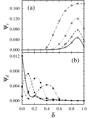
FIG. 6.: Magnitudes of gap equation solutions to the BCS gap equation vs hole density for $J_{3}=J=0.33~{}t$. Shown are (a) $s_{x^{2}+y^{2}}$- and (b) $d_{x^{2}-y^{2}}$-wave gap amplitudes for $t^{\prime}$ values of $0.00~{}t$ (solid lines), $-0.15~{}t$ (dashed lines), $-0.30~{}t$ (dotted lines), and $-0.45~{}t$ (dot-dashed lines). The increase in $\psi_{s}$ in (a) with $t^{\prime}$ is due to the flattening of the energy dispersion at low spin density (large hole density) as well as the narrowing of the band width as negative $t^{\prime}$ increases in value. The $\psi_{d}$ peaks in (b) lie at hole dopings which closely match optimal doping in the materials modeled by the corresponding peaks’ $t^{\prime}$ values.

More interesting results were obtained from the mean field gap calculations where physical values of the variational parameters were used. For $J=0.33~{}t$, there were no significant mixed state solutions found for any values of $\delta$ or $t^{\prime}$, but the $s$- and $d$-wave solutions yielded surprising trends. Figure 6 shows the magnitudes of these solutions to the mean field gap equation over many hole densities and values of $t^{\prime}$. The $s$-wave magnitudes are largest around lower spin density as expected from the Cooper problem results, however the values increase with more negative $t^{\prime}$. This trend of $t^{\prime}$ enhancing $s$-wave seems contrary to the previous results from the dilute limit and Cooper problem, but this incongruent result can be explained by the nature of the energy dispersion. At these low spin densities, the filled states lie close the the energy minimum. As $t^{\prime}$ becomes more negative, the energy dispersion becomes more flat around the minimum, and the band gap reduces in width. These two properties of the energy dispersion become overpowering effects on the $s$-wave gap function’s magnitude for larger values of $\delta$, despite $t^{\prime}$ becoming more negative. This is an expected density-of-states effect, already pointed out by several authors [35, 36].

The $d$-wave magnitudes of Fig. 6(b) are the most striking results of all. The magnitudes are highest closer to half-filling, again as expected from the Cooper problem results, where $\delta$ has values more representative of actual physical superconducting systems. For a given value of $t^{\prime}$, the highest gap function magnitude seems to occur at a hole density representative of optimal doping for the particular superconducting material being modeled by that $t^{\prime}$ value.

For example, the highest gap function magnitude for $t^{\prime}=-0.15~{}t$ occurs at $\delta=0.15$, which is close to optimal doping for La_2-xSr_xCuO₄, whereas for $t^{\prime}=-0.45~{}t$, the highest magnitude lies at $\delta=0.4$, close to optimal doping for YBa₂Cu₃O_7-x.

Further mean field calculations were made with regard to anisotropy. The previous results were all made with tetragonal symmetry, where the relative phase between the $s$- and $d$-wave components of the solutions to the gap equation was found to be $\pi/2$ and $0$ when the starting matrix contained complex and real random values, respectively. The ground state energies for both cases were found to be degenerate, at least for the parameter ranges used in these calculations. When an anisotropic energy dispersion was assumed, namely $\epsilon({\bf k})=-2t_{a}\cos{k_{x}}-2t_{b}\cos{k_{y}}-4t^{\prime}\cos{k_{x}}\cos{k_{y}}$, where $t_{a}\neq t_{b}$, this relative phase between the $s$- and $d$-wave components was only found to be $0$, even when an initial matrix of random complex values was used. As the anisotropy increased, $\psi_{s}$ increased and $\psi_{d}$ decreased, however, both effects were not profound.

A systematic study of the extended $t$-$J$ model has been presented in the last three sections, beginning with a simplistic single-pair model in the dilute limit, followed by evaluation of a single-pair in the Cooper problem, and then ending with a mean field approach. At each step along this evolution, we have shown that $s$- and $d$-wave phases do exist (and indeed co-exist in a mixed fashion), dependent upon the shape and size of the Fermi surface as described by the parameters $t^{\prime}$ and $\delta$. Variational Monte Carlo calculations have already shown the presence of a mixed $s$-$d$ symmetry in the $t$-$J$ model for the case of $t^{\prime}=0$ [18]. A cross-over was seen where the ground state symmetry was pure $d$-wave for $\delta<0.12$ and an admixture of $s$- and $d$-wave for $\delta>0.12$ up to around $\delta=0.4$. Further unpublished calculations show that the addition of the $t^{\prime}$-term decreases and eliminates this mixed phase as $t^{\prime}$ increases in magnitude. The trends derived from the dilute limit, the Cooper problem, and the mean field approach as treated in the $t$-$J$ model have now yielded physical reasons for the results seen in the VMC calculations.

Support for the applicability of the extended $t$-$J$ model in describing the high-temperature superconductors must far more importantly come from experimental evidence for a gap symmetry dependent upon Fermi surface shape and doping. A survey of various experimental work is made in Sec. VII where the case is made for identifying the extended $t$-$J$ model as a detailed material-specific description of superconductivity in the cuprates.

VII Experimental Survey

The calculations reported in this paper identify two trends for the ${\it ground~{}state}$ of high-$T_{c}$ superconductors. There is dependence of the form of the gap function on the dispersion relation quantified by the second-neighbor hopping. There is dependence on the hole concentration. These are parameters which vary considerably from system to system. The theory therefore indicates that not all high-$T_{c}$ superconductors are alike. Experiments on magnetic properties also indicate differences between the different systems; the incommensurability of the short-range order in the La_2-xSr_xCuO₄ system does not appear to be present in the YBa₂Cu₃O₇ system. Similarly, these properties are doping-dependent; the various signatures of the spin gap are present in underdoped, but not optimally doped YBa₂Cu₃O_7-δ. (For a review of magnetic properties, see Ref.  [37].) This section is devoted to a survey of different systems to see if there is experimental support for this point of view. Indeed, a growth of theoretical work has resulted from these recent experimental results, the details of which we present in Sec. VII. According to the above results, we should investigate each separate high-$T_{c}$ for $d$-wave, $s$-wave, and $s$-$d$ mixed wave [38, 39]. The last possibility requires further discussion. $s$-$d$ mixing can occur in two forms: $s$+$id$ and $s$+$d$, depending upon whether the proportionality constant between them does or does not have an imaginary part, respectively. The calculations above do not discriminate between these two possibilities. For recent work on the mixing hypothesis in various models, see Refs. [40, 41]. Variational Monte Carlo calculations, which could in principle show an energy difference in the ground state as a function of the phase difference, were inconclusive [18]. In the $s$+$id$ state there are no nodes in the gap, and time reversal symmetry is broken. Josephson interference experiments put very strong upper limits on the admixture of $s$-wave in any $s$+$id$ state [42]. In addition, the $s$+$id$ state would lead to domain effects which are not observed. (By contrast, the negative results in optical dichroism experiments do not test for the $s$+$id$ state [43].)

In the following discussion, however, we shall concentrate on the $s$+$d$ state as the most likely mixed pairing state, and all references to mixed-wave pairing below are to this state only. In this state the $d$-wave gap nodes, located along the $k_{x}=\pm k_{y}$ directions, move toward the crystal axis $k_{x}=0$ or $k_{y}=0$ as the relative weight of the $s$-component increases. Which of the two directions is chosen depends on the sign of the coupling to the orthorhombic distortion which exists in most high-$T_{c}$ materials. If there is no such distortion, then $s+d$ and $s-d$ are degenerate. If a critical size of the $s$-wave component is reached, then the nodes move together and they annihilate one another. Beyond that point, the system has a “hard” gap; there are no quasiparticle excitations. If the $s$-wave component predominates, the $d$-wave admixture may be thought of as contributing some orthorhombic distortion to a gap with otherwise tetragonal symmetry. Further discussion of the mixed state is found in Ref. [18].

The purpose of this section is to survey what is known about the gap symmetry of different high-$T_{c}$ materials, without making the assumption that the gap symmetry must be the same in all. Previous surveys have often lumped all materials together. This would defeat our purpose of looking for material-specific trends. A more complete survey, but from a different point of view, may again be found in Ref. [20].

The best-studied compound is of course YBa₂Cu₃O₇. It appears from temperature-dependent penetration depth measurements $\lambda(T)$ to be quite clear that there are low energy quasiparticle excitations in this system [3]. This shows that any admixture of $s$-wave must be less than the critical value. Anisotropy in $\lambda$ suggests that pure $d$-wave is not the gap symmetry in this material, but this could also be due simply to the orthorhombic character of the crystal structure.

The Josephson interference experiments of the Illinois and ETH groups measure the difference in the phase of electrons passing through perpendicular faces of a crystal [7, 9]. It is rather accurately measured to be $\pi$, and this is in agreement with independent measurements. This is likely to reflect very well the phase shift under a $90^{\circ}$ rotation in momentum space. It is important to point out that this is consistent with pure $d$-wave or with the $s$+$d$ state, both of which give $\pi$ for this quantity. These experiments rule out the $s$+$id$ state, which has a shift of $\pi/2$ if the two components have equal weight [42]. The IBM tricrystal experiments [8] further show that the nodes in the gap cannot be more than $30^{\circ}$ from the $k_{x}=\pm k_{y}$ points. This puts constraints on the weight of any admixture of $s$-wave. $c$-axis tunneling experiments, on the other hand, would suggest that the $s$-wave component is not negligible [44]. Indeed, if the critical current along this direction is related to the size of the $s$-wave gap, the $s$-wave part is perhaps 10% to 20% of the $d$-wave part. Nuclear magnetic resonance experiments on this material are inconsistent with a pure $s$-wave state, and have often been interpreted in terms of $d$-wave superconductivity [45]. The $s$+$d$ interpretation has not been done; however, the fact that anisotropic $s$-wave [46] and $s$+$id$ [18] theories can account for the data equally well suggests strongly that the observations are consistent with $s$+$d$ as well. Temperature-dependent Raman scattering on YBa₂Cu₃O₇ shows most sensitivity in the $B_{1g}$ geometry [47]. This supports $d$-wave pairing [48, 49]. Some limitation can be placed on the proportion of s-wave from these experiments, but how much is not clear. Quasiparticle (Giaever) tunneling experiments performed by point contacts [50], tend to show the presence of states near the chemical potential, consistent with $d$-wave or $s$+$d$, but it has generally proven to be difficult to unambiguously compare theory and experiment (and even experiment and experiment) in this area. It appears that quasiparticle tunneling performed in conjunction with scanning tunneling microscopy holds out the best hope of gap determination, as surface quality and site specificity are important issues [51]. At present, however, this method gives ambiguous results for the density of states in the superconducting state of YBa₂Cu₃O₇ [52].

[ Y123 B22128 B2212(8+$x$) LSCO NDCO $\lambda(T)$ $d$, $d$+$s$ - - - $s$ Jos. Interf. $d$, $d$+$s$ - - - - Photemiss. - $d$ $d$+$s$ - - NMR $d$, $d$+$s$ - - - - Tunneling $d$ ? $d$ ? - - $s$ Neutr. Scatt. - - - $s$ - $t^{\prime}/t$ -0.4 -0.2 ? -0.2 -0.16 +0.16 ]

TABLE I.: EXPERIMENTAL SURVEY

Using Ginzburg-Landau theory, Berlinsky and Kallin studied the Abrikosov vortex lattice and found that the lattice changes from a triangular to an oblique to a square spacing with increasing field and $sd$-mixing parameter [53]. This may explain neutron scattering experiments in YBa₂Cu₃O₇ [54]. The interesting point about this work from the point of view of this paper is that the $s$-wave component of the order parameter is zero in the absence of current flow. Instead, it is induced by the supercurrent which is itself a response to the applied field [55]. Thus, there does not need to be an actual $s$-wave instability in the (translationally invariant) ground state for the effects of $s$-$d$ mixing to be experimentally observable. It may be sufficient that there exists a phase boundary between pure $d$ wave and and $s$-$d$ mixed phase and that some systems are close to it.

The second material in terms of detailed gap studies is Bi₂Sr₂CaCu₂O_8+x. Its particular interest is that the gap is visible in angle-resolved photoemission. Although this experiment measures only the absolute magnitude of the gap function, it has an angular resolution not available in the Josephson tunneling experiments. Furthermore, $x$ can be varied, and this is of pivotal importance from our point of view, as the prediction that the $s$-wave component can develop as the hole doping ($x$) increases can be tested. The optimally doped compound shows a well-developed gap $\Delta_{x}$ along at least one of the crystal axes (say, $k_{x}=0$), and a very small or zero gap $\Delta_{xy}$ along the diagonal (say, $k_{x}=\pm k_{y}$) [6]. This is in contrast to results in overdoped Bi₂Sr₂CaCu₂O_8+x ($T_{c}=75K$) [5]. Here it is found that there is a gap along the $k_{x}=\pm k_{y}$ direction at lower temperatures, and that the anisotropy ratio $\Delta_{x}/\Delta_{xy}$ is therefore temperature-dependent. This has been successfully analyzed under the hypothesis of $s$+$d$ and is inconsistent with pure $d$-wave [56]. Raman spectroscopy in this compound also supports d-wave pairing, again with no clear limitation on $s$-$d$ mixing [57]. Giaever tunneling experiments are not always consistent with one another in Bi₂Sr₂CaCu₂O_8+x materials, but again often suggest states near the chemical potential. Recent scanning tunneling microscopy experiments have been seen as indicative of an $s$+$d$ state [58], a $d$ state [59], and dependence on surface layer is also observed [60].

Experiments probing gap structure are somewhat harder to come by in other materials. Nd_2-xCe_xCuO₄ has been the subject of experiments measuring the temperature dependence of the penetration depth [4] and the tunneling spectra [61]. Both are consistent with a fully-developed gap of $s$-wave type. Neutron scattering experiments in La_2-xSr_xCuO₄ detect a gap in the $k_{x}=k_{y}$ direction [62]. This experiment is consistent with $s$-wave or $s$+$d$, though the somewhat isotropic suppression of scattering would favor pure $s$-wave, probably of a gapless nature. Impurity scattering in a $d$-wave superconductor can also produce rather isotropic suppression [63]. The tricrystal experiment has recently been performed on a Tl-based film [64]. It also indicates that nodes in the gap of this material must be within $30^{\circ}$ of the diagonals in the Brillouin zone.

We summarize this information in Table I. Also given in the table are values of $t^{\prime}$, the second neighbor hopping element, taken from various sources [65, 66, 67]. The theory would generally predict that $s$-wave should be more likely as one moves to the right in the table, as $t^{\prime}$ decreases in magnitude. The doping is not so easy to estimate, but it is certain that the overdoped Bi₂Sr₂CaCu₂O_8+x has more holes than the optimally doped Bi₂Sr₂CaCu₂O_8+x, and therefore should lie in the table as shown. In general, the trend is indeed toward more $s$-wave behavior on the right hand side of the table, in qualitative agreement with theory.

A common experimental objection to the $s$-$d$ mixed state is that it involves two superconducting transitions, but only one is observed. This subject is treated rather thoroughly in Ref. [18] and we summarize their conclusions here. Symmetry analysis shows that there are two transitions only if the material is tetragonal. In the orthorhombic case, $s$-wave and $d$-wave have the same transformation properties under the operations of the point group and only one transition will occur. In UPt₃, the only material in which two superconducting transitions are known to occur as a function of temperature, they are visible in specific heat measurements and in ultrasonic absorption and velocity measurements. In high-$T_{c}$ systems, the transition in specific heat has been clearly seen only in YBa₂Cu₃O₇, which is quite orthorhombic. In the nearly-tetragonal Bi-based and Tl-based systems, the appropriate measurements have not been done.

VIII Conclusion

The calculations presented in this paper use the simple mean-field method for the investigation of superconductivity. There is, in practice, little choice of methods if the Hamiltonian has a form which is flexible enough to show material-specific behavior. (See, for example, Eq. (132).) More sophisticated methods, such as slave-boson methods with gauge fluctuations, have been developed for the investigation of $t$-$J$-type models, but these are quite difficult to handle even for the simplest models. Finite-size calculations are limited to lattices whose linear dimensions are comparable to, or smaller than, a coherence length. Quantum Monte Carlo (QMC) calculations (again on simpler models than the current one) have severe sign problems in the regimes of interest. VMC calculations may be possible, but this is left for future investigation. To the extent that we have been able to compare our results with the VMC results, there is qualitative agreement. Finally, our calculations in the spin-interaction model are cruder than the strong-coupling calculations which have been done in the spin-fluctuation model. The spin-interaction model is genuinely microscopic, however, not semiphenomenological. Compensating for the disadvantage of the approximate treatment of interactions is the advantage that the method is physically transparent - the reasons for the trends which appear are all evident, and much of the paper has been devoted to the explanation of these trends. This transparency is not always a feature of highly numerical methods such as QMC or VMC.

Thus the trends towards $d$-wave with increasing $t^{\prime}$ can be seen as softening angular variations in the pair wavefunction, whereas the trend towards $s$-wave with increasing doping is seen as due to a relaxation of phase-space restrictions. The trend towards higher optimal doping with increasing $t^{\prime}$ is a density-of-stated effect. There is evidence for all of these effects in experiments. The most dramatic of these is the change from strong $d$-wave in YBa₂Cu₃O₇ to $s$-wave in Nd_2-xCe_xCuO₄.

This analysis allows us to evaluate qualitatively the actual relevance of the calculations to real materials. For example, let the ideal Fermi surface of the Cooper problem be replaced by the actual momentum distribution. The latter will be much flatter, with a relatively small discontinuity at the Fermi surface (assuming a Fermi liquid normal state) or no discontinuity (Luttinger liquid normal state). Therefore the phase space restrictions will be weaker in the real system. This would favor $s$-wave and move the crossing point of $s$-wave and $d$-wave at $n=0.55$ (at $t^{\prime}=0$) in Fig. 4 to higher values with increasing $t^{\prime}$. Relaxation of the very large $U$ (strong short range Coulomb interaction) approximation will also favor $s$-wave, as the constraint of absolutely no double-occupancy has no effect on $d$-wave, whereas it suppresses $s$-wave pairing. By the same token, the neglect of the long range Coulomb interaction in our model probably prejudices our results toward $d$-wave. The usual frequency-mismatch arguments so important for superconductivity with electron-phonon interaction do not apply here, since all interactions are instantaneous. It is precisely for that reason that our results fly in the face of conventional wisdom that magnetic mechanisms can lead only to $d$-wave pairing. In the absence of a cutoff in the interaction, all of momentum space comes into play, and the kinetic energy of the pair plays an important role. This brings $s$-wave superconductivity into the picture.

The trends which arise from our simple analysis of this flexible model appear to describe some of the otherwise puzzling and contradictory results on different high-$T_{c}$ materials. They show that the ground state of different materials may be different in the context of a magnetic mechanism.

We would like to thank T. M. Rice, S. Hellberg, A. Sudbø, M. Ma, P.W. Anderson and M. Randeria for useful discussions and correspondence. This work was supported by the National Science Foundation through Grant DMR-9214739 and by NORDITA, Copenhagen, Denmark

REFERENCES

- [1]
- [2]
- [3] W.N. Hardy, D.A. Bonn, D.C. Morgan, R. Liang, and K. Zhang, Phys. Rev. Lett. 5, 3999 (1993).
- [4] S. Anlage et al., Phys. Rev. B 50, 523 (1994).
- [5] J. Ma, C. Quitmann, R.J. Kelley, H. Berger, G. Margaritondo, M. Onellion, Science 267, 862 (1995).
- [6] Z.-X. Shen et al.. Phys. Rev. Lett. 70, 1553 (1993).
- [7] D.A. Wollman et al., Phys. Rev. Lett. 71, 2134 (1993); ibid., 73, 1872 (1994); ibid., 74, 797 (1994).
- [8] J.R. Kirtley et al., Nature 373, 225 (1995).
- [9] D.A. Brawner and H.R. Ott, Phys. Rev. B 50, 6530 (1994).
- [10] K. Miyake, S. Schmit-Rink, and C.M. Varma, 34, 6554 (1986).
- [11] M.T. Béal-Monod, C. Bourbonnais, and V.J. Emery, Phys. Rev. B 34, 7716 (1986).
- [12] A. Ruckenstein, P.J. Hirschfeld, and J. Appel, Phys. Rev. B 36, 857 (1987).
- [13] C. Gros, R. Joynt, and T.M. Rice, Z. Phys. B 68, 425 (1987).
- [14] N.E. Bickers, D.J. Scalapino, and R.T. Scalettar, Internat. J. Mod. Phys. B1, 687 (1987)
- [15] T. Moriya, Y. Takahashi, and K. Ueda, J. Phys. Soc. Japan 59, 2905 (1990).
- [16] P. Monthoux, A. Balatsky, and D. Pines, Phys. Rev. B 46, 14803 (1992).
- [17] J.R. Schrieffer, X.-G. Wen, and S.-C. Zhang, Phys. Rev. Lett. 60, 944 (1988);J.R. Schrieffer, X.-G. Wen, and S.-C. Zhang, Phys. Rev. Lett. 61, 2814 (1988);J.R. Schrieffer, X.-G. Wen, and S.-C. Zhang, Phys. Rev. 42, 7967 (1989);
- [18] Q.P. Li, B.E.C. Koltenbah, and R.J. Joynt, Phys. Rev. B 48, 437 (1993).
- [19] K.A. Muller, Nature 377 133 (1995).
- [20] D.J. Scalapino, Phys. Repts. 250, 331 (1995).
- [21] E. Dagotto, Rev. Mod. Phys. 66, 763 (1994).
- [22] W. von der Linden, Phys. Repts 220, 53, (1992)
- [23] B.E.C. Koltenbah and R. Joynt, unpublished.
- [24] C. O’Donovan and J, Carbotte, Phys. Rev. B 52 16208 (1995).
- [25] M.T. Béal-Monod and K. Maki, Phys. Rev. B 53 5775 (1996).
- [26] G. Varelogiannis, preprint, cond-mat/9509154.
- [27] A. Nazarenko, S. Haas, J. Riera, A. Moreo, and E. Dagotto, preprint, cond-mat/9603046.
- [28] F.C. Zhang and T.M. Rice, Phys. Rev. B 37, 3759 (1988).
- [29] C. Gros, R. Joynt, and T.M. Rice, Phys. Rev. B 36, 381 (1987).
- [30] A.J. Leggett, in Modern Trends in Condensed Matter, edited by A. Pekalski and J. Przystawa (Springer, Berlin, 1980).
- [31] K. Miyake, Prog. Theor. Phys. 69, 1794 (1983).
- [32] M. Randeria, J. Duan, and L. Shih, Phys. Rev. Lett. 62, 981 (1989).
- [33] C.S. Hellberg and E. Manousakis, Phys. Rev B 52, 4639 (1995).
- [34] M.Y. Kagan and T.M. Rice, J. Phys. : Condens.. Matter, 6, 3771 (1994).
- [35] E. Dagotto, et al., Phys. Rev. B 49 3548 (1994).
- [36] D.M. Newns, C.C. Tsuei, P.C. Pattnaik, Phys. Rev. B 52, 13611 (1995); S. Markiewicz, J. Phys. Condens. Matt. 2, 6223 (1990); A.A. Abrikosov, et al. , Physica C 214, 73 (1993).
- [37] A.P. Kampf, Phys. Repts. 249, 219 (1994)
- [38] G. Kotliar, Phys. Rev. B 37, 3664 (1988).
- [39] G.J. Chen, F.C. Zhang, C. Gros, and R. Joynt, Phys. Rev. B 42, 2662 (1990).
- [40] C. O’Donovan and J. Carbotte, Physica C 252, 87 (1995).
- [41] K. Musaelian, J. Betouras, A.V. Chubukov, and R. Joynt, Phys. Rev. B 53, 3598 (1996).
- [42] D. van Harlingen, Rev. Mod. Phys. 67, 515 (1995).
- [43] Q.P. Li and R. Joynt, Phys. Rev. B 44, 4720 (1991).
- [44] A.G. Sun, D.A. Gajewski, M.B. Maple, and R.C. Dynes Phys. Rev. Lett. 72, 2267 (1994).
- [45] N. Bulut, D. Hone, D. Scalapino, and N. Bickers, Phys. Rev. Lett. 64, 2723 (1990); H. Monien and D. Pines, Phys. Rev. B 41, 6297 (1990), The experiments are reviewed by C. Pennington and C. Slichter, in Physical Properties of High Temperature Superconductors II, ed. D. Ginsberg (World Scientific, Singapore, 1990), and R. Walstedt and W. Warren, Science 248, 1082 (1990).
- [46] S. Chakravarty, A. Sudbø, P.W. Anderson, and S. Strong, Science 261, 337 (1993).
- [47] R. Hackl et al., Phys. Rev. B 38, 7133 (1988).
- [48] H. Monien and A. Zawadowski, Phys. Rev. Lett. 63, 911 (1989).
- [49] T.P. Devereaux, A. Virosztek, and A. Zawadowski, Phys. Rev. B 51, 7133 (1995).
- [50] J.M. Valles et al., Phys. Rev. B 44, 11986 (1991); H. Edwards et al., Phys. Rev. Lett. 69, 2967 (1992); T. Miller et al., Phys. Rev. B 48, 7499 (1993).
- [51] K. Kitazawa, Science 271, 313 (1996).
- [52] M. Nantoh et al., J. Appl. Phys. 75, 5227 (1994).
- [53] A.J. Berlinsky and C. Kallin, Phys. Rev. Lett. 75 2200 (1995).
- [54] B. Keimer et al., J. Appl. Phys. 76, 6778 (1994).
- [55] R. Joynt, Phys. Rev. B 41, 4271 (1990).
- [56] J. Betouras and R. Joynt, Europhys. Lett. 31, 119 (1995).
- [57] T.P. Devereaux et al., Phys. Rev. Lett. 72, 396 (1994).
- [58] K. Ichimura, K. Suzuki, K. Nomura, and S. Takekawa, J. Phys.: Condens. Matt. 7, L545 (1995).
- [59] Ch. Renner and Ø. Fischer, Phys. Rev. B 51, 9208 (1995).
- [60] H. Murakami and R. Aoki, J. Phys. Soc. Japan 64, 1287 (1995).
- [61] Q. Huang et al., Nature 347, 369 (1990).
- [62] T.E. Mason, G. Aeppli, S.M. Hayden, A.P. Ramirez, and H.A. Mook, Phys. Rev. Lett. 71, 919 (1993).
- [63] S.M. Quinlan and D.J. Scalapino, Phys. Rev. B 51, 497 (1995).
- [64] C.C. Tsuei, et al., Science 271, 329 (1996).
- [65] For YBCO as derived by T. Tohyama and S. Maekawa, Phys. Rev. B 49, 3596 (1994). A detailed explanation of how is derived from band structure is given in this reference as well.
- [66] For LSCO and for NCCO as cited by H. Fehske and M. Deeg, Jour. of Low Temp. Phys. 99 425 (1995).
- [67] For BSCCO we derive from a tight-binding fit to the measured energy dispersion in Fig. 3 of D.S. Dessau, et al., Phys. Rev. Lett. 71 2781 (1993).