Resonance in One–Dimensional Fermi–Edge Singularity.

Abstract

The problem of the Fermi–edge singularity in a one–dimensional Tomonaga–Luttinger liquid is reconsidered. The backward scattering of the conduction band electrons on the impurity–like hole in the valence band is analyzed by mapping the problem onto a Coulomb gas theory. For the case when the electron–electron interaction is repulsive the obtained exponent of the one–dimensional Fermi–edge singularity appears to be different from the exponent found in the previous studies. It is shown that the infrared physics of the Fermi–edge singularity in the presence of backward scattering and electron–electron repulsion resembles the physics of the Kondo problem.

I Introduction

Large optical singularities in the absorption and emission spectra have been observed by Calleja et. al. [2] in semiconductor quantum wire structures in the extreme quantum limit when only the lowest one–dimensional (1–d) subband is occupied by electrons. The pronounced features in the optical spectra have been interpreted as strong Fermi–edge singularities (FES) of the 1–d electron gas. The FES arises (e.g. for absorption), because the optical process is accompanied by a multiple scattering of the conducting electrons on a hole in the valence band, which is created at the absorption of the electro–magnetic wave and acts as an impurity–like center. In the case of 1–d geometry the scattering of the conducting electrons by the hole is limited to scattering in the forward or backward directions. Another special feature is related to the electron–electron interaction in 1–d. In contrast to higher dimensions, the 1–d electron gas can not be treated as an ordinary Fermi liquid even when the electron–electron interaction is small. The experiment [2] initiated a number of papers discussing the FES in 1–d metallic systems for the forward scattering [3, 4] and the backward one [5, 6, 7, 8] in the presence of the electron–electron interaction.

In the present paper the effect of the backward scattering on the FES in 1–d will be reconsidered. The exponent of the 1–d FES obtained here appears to be different from the one that was found in Ref.’s [5, 6, 7, 8]. It is shown that the infrared physics of the Fermi–edge singularity in the presence of backward scattering together with electron–electron repulsion resembles the physics of the Kondo problem. This aspect of the problem was missed in the preceding studies.

FES or Mahan singularity is a power law singularity in the electro–magnetic wave absorption (or emission) coefficient when the frequency is close to the Fermi energy [9]. That is in contrast to a naive expectation that the absorption coefficient is zero bellow the Fermi energy and is proportional to the density of states of the conduction band above the Fermi energy. Since in common metals the FES is observed in the $X$–ray range, it is also called sometimes the $X$–ray singularity. The singularity arises because the absorption is accompanied by the infrared catastrophe phenomena. When the electro–magnetic wave is absorbed, an electron from a deep level is excited to the conduction band and, correspondingly, a hole is created deep in the valence band. The abrupt appearance of the scattering potential of the deep hole leads to excitation of an infinite number of low energy electron–hole pairs in the conduction band. Besides, the electron excited from the deep level to the conduction band scatters multiply on the hole. The latter process, which includes an exchange with other electrons of the conduction band, leads to enhancement of the absorption coefficient. The physical reason of this enhancement is the increase of the effective density of states near the deep hole due to its attraction of electrons. On the other hand the creation of the electron–hole pairs in the conduction band reflects the fact that the final state of the electrons in the presence of the deep hole potential is orthogonal to the initial state. This process is called the orthogonality catastrophe of Anderson [10] and it leads to a reduction of the absorption coefficient. The value of the exponent of the FES is determined by these two competing effects.

The effects related to the physics of the FES can be found in various situation where a sudden change of a scattering potential happens. The well known example is the Kondo problem describing scattering of conduction electrons on a magnetic impurity. When the impurity spin is flipped the impurity potential on which the conduction electrons are scattered is abruptly altered. Therefore, the Kondo problem can be treated [11] as a response of the electrons on a sequence of sudden changes of the local scattering potential. The problem can be mapped on a classical Coulomb gas theory of alternating positive and negative charges (spin flips) with logarithmic interaction. In the present paper it will be shown that the FES problem in 1–d can also be analyzed by mapping it on a Coulomb gas theory, similarly to the Kondo problem.

To calculate the exponent of the FES it is needed to sum a series of infrared–divergent logarithmic terms. A corresponding theory was developed for three dimensional metals (3–d) by Noziéres and collaborators in a series of papers [12, 13, 14]. The recoil of the hole, due to its finite mass, together with Auger processes lead to a natural cutoff of the infrared singularities. It is usually assumed, for simplicity, at the discussion of the FES that these effects can be neglected. The other common assumption is that the potential created by the deep hole is a short range one. That is because the electron screening develops on short scales, while at studies of infrared phenomena large distances are essential. Since in 3–d metals the Fermi liquid parameters are determined by the short scale physics, it is also generally assumed that one can use the Fermi liquid description for the conduction electrons at the consideration of the FES.

At studies of the FES in 1–d the role of these common assumptions may change. It has been noticed [3] that in 1–d systems the recoil of the deep hole does not suppress the FES, at least for the forward scattering. Here we will ignore the recoil effects completely as well as the Auger processes. In this paper we will also not discuss the problem of screening of the potential of the deep hole, despite that it may be essential for the FES in modulation–doped quantum wires. Since we are mainly interested now in the effects of the $2k_{F}$–backward scattering, it will be assumed that the potential of the deep hole is local. The most intriguing aspect of FES in 1–d is related to the role of the electron–electron interaction. In some sense the Fermi surface is weakened in 1–d as a result of the interaction of electrons. In the case of the Tomonaga–Luttinger model the jump in the occupation numbers of electrons at the Fermi energy is replaced by a singularity, and there are no single electron quasi–particles [15, 16, 17]. Since the FES is a Fermi surface effect, the investigation of the role of the electron–electron interaction in this problem is of clear interest.

The effective way to investigate the infrared properties of the 1–d electron systems is the bosonization technique. In fact, the important step in the developing of this technique was made just in connection with the problem of the FES. Schotte and Schotte extended the approach of Ref. [15] and developed a very compact and economical description of the FES for $s$-wave scattering in 3–d [18]. In the present paper the consideration of the electrons interaction will be confined to the Tomonaga–Luttinger model where it is assumed that the electrons do not scatter backward in the course of the electron–electron interactions. Since Tomonaga–Luttinger model has a simple solution in the bosonization technique, it is natural to apply that technique for finding the FES in 1–d in the presence of interactions between the electrons.

In the case when at the scattering on the potential of the hole in the valence band the electrons are scattered only in the forward direction, the FES can be found [3] following the Schotte and Schotte method. For completeness of the presentation and with the purpose of introducing notations we have reconsidered this case in Sec. II A. When the backward scattering on the hole potential is included, it is shown in Sec. II B that the problem can be mapped on a gas of charged particles, similarly to the Coulomb gas mapping in the Kondo problem [11, 19, 20]. The role of the spin flip in the Kondo problem acts now the change of the electron motion from left to right and visa versa at the backward scattering on the hole. In comparison with the Kondo problem the Coulomb gas describing the 1–d FES is different in two aspects. In the $S=\frac{1}{2}$ Kondo problem successive flips should follow alternatively, while in the case of FES there is no limitations on the order of left–right and right–left scattering. (In the end of Sec. IV a certain relationship of the non alternating Coulomb gas with the two–channel Kondo problem is outlined.) The other difference is due to the creation of the additional electron in the conduction band at the absorption of the electro–magnetic wave. This gives rise to two additional charges located at the ends of the Coulomb gas system. In the case of repulsion of electrons the gas of the charged particles is in the hot plasma phase. Therefore a new scale — the screening radius of the plasma — is generated in this problem as a combined effect of the backward scattering and the interaction. The shape of the absorption line for frequencies close enough to the Fermi–edge is controlled by this scale. The reduction of the 1–d FES problem to the classical gas theory yields a value of the FES exponent in the vicinity of the Fermi edge, which is different from the one obtained in preceding studies [5, 6, 7, 8].

In section III the FES is analyzed using fields, which where first introduced in Ref. [7]. In that representation the scattering is simplified, but at a price that the electron–electron interaction is described by a non–local theory of self–dual fields. A special treatment is needed in case of such a theory. The renormalization group analysis of the problem using these variables is elaborated in Sec. III B. In addition, an iteration procedure is developed in Sec. III C for the analysis of the FES problem. This procedure is useful for determining the screening length of the Coulomb gas in the hot plasma phase.

To understand the obtained exponent of the FES, in Sec. IV the result is interpreted in terms of the phase shift theory of Noziéres and De Dominicis [14]. It is argued that the discrepancy between the value of the FES exponent obtained in the present paper and the result of Ref.’s [5, 6, 7, 8] is because in these papers the asymptotic regime of the problem is described by a weak link junction. However, two weakly connected wires represent a system with strong depletion of the density of electrons at the defect center. It is shown in the end of Sec. IV that the use of such system as the asymptotic limit description of a weak impurity scatterer, as it was suggested in the theory of Ref. [21, 22], is in contradiction with the Friedel sum rule. In fact, it is concluded here that the infrared asymptotic regime of the FES resembles to the Kondo resonance.

II Coulomb gas

In this section we show that in 1-d systems the correlation function $F(t)$ determining (after the Fourier transform) the Fermi edge singularity can be presented as a product of two terms. The first one is related to the forward scattering of the conduction electrons by the hole, which is created in the valence band at the absorption of the external electro–magnetic wave. This term can be calculate directly, while the second one describing the backward scattering by the hole, is analyzed by mapping onto a Coulomb gas. This approach allows us to find the behavior of $F(t)$ at asymptotically large time. For compactness we confine the consideration bellow to a spinless case, and the spin degrees of freedom of the conduction electrons are included in the appendix (A).

A The forward scattering

The Hamiltonian describing the 1-d electron liquid is given by

$$H_{0}=iv_{F}\int dx\psi^{\dagger}_{R}(x)\frac{\partial}{\partial x}\psi_{R}(x)-iv_{F}\int dx\psi^{\dagger}_{L}(x)\frac{\partial}{\partial x}\psi_{L}(x)+\frac{1}{2}V\int dx\left(\rho_{R}(x)+\rho_{L}(x)\right)^{2},$$ (1)

where $\psi_{R}(x)\mbox{ and }\psi^{\dagger}_{R}(x)$ are the field operators of fermions that propagate to the right with wave vectors $\approx+k_{F}$, and $\psi_{L}(x)\mbox{ and }\psi^{\dagger}_{L}(x)$ are the field operators of left propagating fermions with wave vectors $\approx-k_{F}$; $\;\rho_{L\left(R\right)}(x)=\psi^{\dagger}_{L(R}(x)\psi_{L\left(R\right)}(x)$ are the electron density operators; the spectrum of the electrons is linearized near the Fermi points and $v_{F}$ is the Fermi velocity; $V$ describes the density–density interaction with momentum transfers much smaller than $k_{F}$. Hamiltonian (1) corresponds to the Tomonaga–Luttinger model, which describes the 1-d electron liquid when the backward scattering amplitude of the electron-electron interaction may be ignored. Eq. (1) is a fixed point Hamiltonian for a broad class of 1-d systems.

After the absorption of the external electro–magnetic wave a hole is created in the valence band together with an additional electron in the conduction band. It will be assumed hereafter that the position of the hole is fixed at $x=0$. The scattering of the conduction band electrons by this hole is given by

$$H_{sc}=U(k=0)\left(\psi_{R}^{\dagger}(0)\psi_{R}(0)+\psi^{\dagger}_{L}(0)\psi_{L}(0)\right)+U(2k_{F})\psi^{\dagger}_{R}(0)\psi_{L}(0)+U^{*}(2k_{F})\psi^{\dagger}_{L}(0)\psi_{R}(0),$$ (2)

where $U(k)$ are the Fourier transform amplitudes of the hole potential $U(x)$, and $\psi_{R(L)}(0)=\psi_{R(L)}(x=0)$. Thus, $U(k=0)$ is the forward scattering amplitude and $U(2k_{F})=-|U(2k_{F})|e^{i\varphi_{u}}$ is the backward one.

In order to find the electro–magnetic wave absorption line shape $I(\omega)$ one needs to calculate the Fourier transform of the correlation function [14, 18]

$$F(t)=\left<e^{iH_{0}t}\psi(0)e^{-iH_{f}t}\psi^{\dagger}(0)\right>,$$ (3)

where $\psi^{\dagger}(0)$ refers to an electron which is created in the conduction band at the absorption, and $H_{f}=H_{0}+H_{sc}$ is the Hamiltonian describing the electron liquid after the creation of the hole. It has been shown in the seminal paper of Schotte and Schotte [18] that bosonic representation of the fermion operators in Eq. (3) gives an illuminating approach for understanding the FES in the case of $s-$wave scattering by the hole. It is natural to apply this approach for the analysis of the FES in 1-d conductors.

It is well known [15] that the bosonization technique (for review see [23, 24]) allows to reduce the Tomonaga–Luttinger Hamiltonian to a quadratic form in terms of operators of bosonic fields $\phi_{0}$ and $\tilde{\phi}_{0}$:

$$\phi_{0}(x) = \frac{-i}{\sqrt{4\pi}}\frac{2\pi}{L}\sum_{p}\frac{\exp\left({-\eta|p|/2-ipx}\right)}{p}\left[\rho_{R}(p)+\rho_{L}(p)\right],$$ (5)

$$\tilde{\phi}_{0}(x) = \frac{-i}{\sqrt{4\pi}}\frac{2\pi}{L}\sum_{p}\frac{\exp\left({-\eta|p|/2-ipx}\right)}{p}\left[\rho_{R}(p)-\rho_{L}(p)\right],$$ (6)

where $\eta^{-1}$ is an ultraviolet cutoff, which is of the order of the conduction band width, and $L$ is the system length. The fields $\phi_{0}$ and its dual partner $\tilde{\phi}_{0}$ are conjugate variables, i.e.,

$$\left[\frac{d\phi_{0}(x)}{dx},\tilde{\phi}_{0}(y)\right]=i\mathchoice{{\hbox{\boldmath$\displaystyle\delta$}}}{{\hbox{\boldmath$\textstyle\delta$}}}{{\hbox{\boldmath$\scriptstyle\delta$}}}{{\hbox{\boldmath$\scriptscriptstyle\delta$}}}(x-y).$$ (7)

After rescaling the operators

$$\phi=\frac{\sqrt{4\pi}}{\beta}\phi_{0},\;\tilde{\phi}=\frac{\beta}{\sqrt{4\pi}}\tilde{\phi}_{0},$$ (8)

the bosonized representation of Hamiltonian (1) becomes

$$H^{B}_{0}=\frac{1}{2}v_{F}\alpha\int dx\left(\left(\frac{d\phi}{dx}\right)^{2}+\left(\frac{d\tilde{\phi}}{dx}\right)^{2}\right),$$ (9)

where

$$\alpha=\frac{4\pi}{\beta^{2}},\;\beta^{2}=4\pi\sqrt{\frac{1-\gamma}{1+\gamma}}\mbox{ and }\gamma=\frac{V}{\left(2\pi v_{F}+V\right)}.$$ (10)

In the bosonization technique [23, 24] the bosonic representations of the operators $\psi_{R}$ and $\psi_{L}$ are given as

$$\psi^{B}_{R}(x) = \frac{e^{ik_{F}x}}{\sqrt{2\pi\eta}}\exp{\left[-\frac{i}{2}\left(\frac{4\pi}{\beta}\tilde{\phi}+\beta\phi\right)\right]}$$ (12)

$$\psi^{B}_{L}(x) = i\frac{e^{-ik_{F}x}}{\sqrt{2\pi\eta}}\exp{\left[-\frac{i}{2}\left(\frac{4\pi}{\beta}\tilde{\phi}-\beta\phi\right)\right]}.$$ (13)

Then, the scattering by the hole may be written in terms of the $\phi$-field as

$$H^{B}_{sc}=\frac{1}{2}v_{F}\left(\frac{\beta\delta_{+}}{\pi}\left.\frac{d\phi}{dx}\right|_{x=0}-\frac{2\delta_{-}}{\pi\eta}\cos(\beta\phi(0)+\varphi_{u})\right),$$ (14)

where the dimensionless amplitudes $\delta_{+}=\frac{U(k=0)}{v_{F}}\mbox{ and }\delta_{-}=\left|\frac{U(2k_{F})}{v_{F}}\right|$ are introduced and $\varphi_{u}=\arg\left(-\frac{U(2k_{F})}{v_{F}}\right)$.

In Eq. (14) the term related to the forward scattering is linear in $\phi$. Therefore, a canonical transformation that shifts at the point $x=0$ the operator $\phi^{\prime}(x)=\frac{d\phi}{dx}$ can be exploited to exclude the forward scattering. Since

$$e^{ia\tilde{\phi}(0)}\phi^{\prime}(x)e^{-ia\tilde{\phi}(0)}=\phi^{\prime}(x)+a\mathchoice{{\hbox{\boldmath$\displaystyle\delta$}}}{{\hbox{\boldmath$\textstyle\delta$}}}{{\hbox{\boldmath$\scriptstyle\delta$}}}{{\hbox{\boldmath$\scriptscriptstyle\delta$}}}(x),$$ (15)

the transformed Hamiltonian $\tilde{H}_{f}^{B}=e^{ia\tilde{\phi}(0)}\left(H_{0}^{B}+H_{sc}^{B}\right)e^{-ia\tilde{\phi}(0)}$ will not contain the forward scattering term, if $a=-\frac{1}{2\pi}\frac{\beta}{\alpha}\delta_{+}$. In the absence of the backward scattering the correlation function $F(t)$, after carrying out the unitary transformation ${\hat{\cal U}}(0)=\exp\left(\frac{i}{2\pi}\frac{\beta}{\alpha}\delta_{+}\tilde{\phi}(0)\right)$, becomes:

$$F(t)_{forward}=\left<\exp\left(iH_{0}^{B}t\right)\psi(0)\hat{\cal U}(0)\exp\left(-iH_{0}^{B}t\right)\hat{\cal U}(0)^{-1}\left(\psi(0)\right)^{\dagger}\right>.$$ (16)

The calculation of $F(t)_{forward}$ can be reduced to a Gaussian–like integral if the bosonic representation (10) for the operators $\psi(0)$, $\psi^{\dagger}(0)$ is applied. Let us choose the component $\psi_{R}(0)$ for the operator $\psi(0)$; the contribution of the other component is equal. Then, the use of the bosonic representation gives:

$$F(t)_{forward}=\left<e^{-i\frac{1}{2}\beta\phi(x=0,t)}e^{-i\frac{1}{2}\tilde{\beta}\tilde{\phi}(x=0,t)}e^{i\frac{1}{2}\tilde{\beta}\tilde{\phi}(x=0,0)}e^{i\frac{1}{2}\beta\phi(x=0,0)}\right>,$$ (17)

where $\tilde{\beta}=\frac{4\pi}{\beta}-\frac{\delta_{+}\beta}{\pi\alpha}$, and the operators $\phi(t)$ and $\tilde{\phi}(t)$ depend on time as $\hat{O}(x,t)=e^{iH_{0}^{B}t}\hat{O}(x,t=0)e^{-iH_{0}^{B}t}$. Now, the standard application of the Baker-Hausdorff formula $e^{A}e^{B}=e^{A+B}e^{\frac{1}{2}[A,B]}$ together with the Gaussian averaging $\left<e^{iA}\right>=e^{-\frac{1}{2}\left<A^{2}\right>}$ yield

$$F(t)_{forward}=e^{-\frac{1}{4}\beta^{2}{\cal G}_{phi}(t)-\frac{1}{4}\tilde{\beta}^{2}{\cal G}_{\tilde{\phi}}(t)},$$ (18)

where ${\cal G}_{\phi}(t)=\left<\phi(0,t)\phi(0,0)-\phi(0,0)^{2}\right>$ is the Green function of the $\phi$–operators, and ${\cal G}_{\tilde{\phi}}$ is defined similarly. It has also been assumed here that $\left<\tilde{\phi}(t)\phi(0)\right>=\left<\phi(t)\tilde{\phi}(0)\right>=0$, what agrees with Eqs. (II A). From Eqs. (II A) and (9) it can be obtained for asymptotically large time

$${\cal G}_{\phi}(t)={\cal G}_{\tilde{\phi}}(t)=\frac{1}{2\pi}\log\left(1+i\frac{\alpha v_{F}t}{\eta}\right).$$ (19)

Finally one gets:

$$F_{forward}\sim\left(\frac{1}{t}\right)^{1-\alpha_{forward}}\;\;\;\;\;\;\alpha_{forward}=1-\frac{1}{8\pi}\left(\tilde{\beta}^{2}+\beta^{2}\right)$$ (20)

and correspondingly the absorption line shape $I(\omega)\sim\left(\delta\omega\right)^{-\alpha_{forward}}$, where $\delta\omega=\omega-\omega_{threshold}$ and

$$\alpha_{forward}=\left(1-\frac{1}{\sqrt{1-\gamma^{2}}}\right)+\frac{\delta_{+}}{\pi}\sqrt{\frac{1-\gamma}{1+\gamma}}-\frac{\delta_{+}^{2}}{2\pi^{2}}\left(\sqrt{\frac{1-\gamma}{1+\gamma}}\right)^{3}.$$ (21)

Here the first term reflects the Luttinger–liquid behavior of the 1–d electrons in the presence of an electron–electron interaction [16, 17]. Note that contrary to the noninteracting case the last term in Eq. (21), which corresponds to the Anderson orthogonality catastrophe, is not the half of the square of the second term.

The above procedure was elaborated by Schotte and Schotte [18] for consideration of the FES in 3-dimensional case for $s$-wave scattering. For the 1–d case the function $F_{forward}(t)$, including the spin degrees of freedom, has been obtained recently in Ref. [3] (see bellow Eq. (A10) for comparison).

B The backward scattering

In the presence of the backward scattering the correlation function $F(t)$ will be studied in the interaction representation with respect to $\tilde{H}^{B}_{b-sc}$:

$$F(t)=\left<\exp\left(iH_{0}^{B}t\right)\psi(0)\hat{\cal U}(0)\exp\left(-iH_{0}^{B}t\right){\cal T}\exp\left(-i\int_{0}^{t}\tilde{H}_{b-sc}^{B}(t^{\prime})dt^{\prime}\right)\hat{\cal U}(0)^{-1}\left(\psi(0)\right)^{\dagger}\right>,$$ (22)

where ${\cal T}$ is the time ordering symbol and the backward scattering term is

$$\tilde{H}_{b-sc}^{B}=-\frac{v_{F}\delta_{-}}{\eta\pi}\hat{\cal U}(0)^{-1}\cos\left(\beta\phi(0)+\varphi_{u}\right)\hat{\cal U}(0).$$ (23)

(The action of the electron–electron interaction, unlike the backward scattering term, is not limited to the interval $[0,t]$. Therefore, electron transitions not only within this time interval contribute to the FES. Fortunately, in the case of the Tomonaga–Luttinger model the renormalization of the fields $\phi$ and $\tilde{\phi}$ by Eq. (8) takes that complications into consideration, and Eq. (22) holds.) When an expansion of the ${\cal T}$-exponential in $\tilde{H}_{b-sc}^{B}(t^{\prime})$ is performed, the result can be written as a sum of all possible time–ordered products of the exponentials of the operators $\pm i\left[\beta\phi(x=0,t^{\prime})+\varphi_{u}\right]$. The averaging procedure of each term in this sum can be easily performed using repeatedly the Baker–Hausdorff formula. This is a standard way of a reduction of the quantum problem of such kind to the physics of classical charged gases; see for example Refs. [19, 20, 25, 26].

Now a subtle point related to the application of the Baker–Hausdorff formula should be commented. Eq. (7) determines the commutation relations of $\phi$ and $\tilde{\phi}$ only up to a constant:

$$\left[\phi(x),\tilde{\phi}(0)\right]=i\int^{x}\mathchoice{{\hbox{\boldmath$\displaystyle\delta$}}}{{\hbox{\boldmath$\textstyle\delta$}}}{{\hbox{\boldmath$\scriptstyle\delta$}}}{{\hbox{\boldmath$\scriptscriptstyle\delta$}}}(x^{\prime})dx^{\prime}=i\frac{1}{2}\mbox{ sign }(x)+C.$$ (24)

This constant may be fixed by the requirement that the representation (10) should ensure the fermion commutation relations of the operators $\psi^{B}_{L}$ and $\psi^{B}_{R}$. That requirement leads to $C=\pm\frac{i}{2}$. In Eq. (14) the cosine of the backward scattering term has been written with $C=-\frac{i}{2}$. Now, using the fact that in $F(t)$ the creation and annihilation operators of the right and left moving electrons appear in equal numbers for non vanishing terms, one can check in a formal way that $C$ does not influence $F(t)$. For that reason it will be assumed hereafter that

$$\left[\phi(0),\tilde{\phi}(0)\right]=0,$$ (25)

what is in correspondence with a naive treatment of this commutator with representation (II A). Consequently, when the Gaussian averaging is performed in the calculation of the correlation function $F(t)$ it may be assumed that

$$\left<\tilde{\phi}(t)\phi(0)\right>=\left<\phi(t)\tilde{\phi}(0)\right>=0,$$ (26)

Usually the correlation function of $\phi$ and $\tilde{\phi}$ operators controls the relative phase of certain operators when they exchange their coordinates, because

$$\left<\tilde{\phi}(x,i\tau)\phi(y,i\tau^{\prime})\right>=\frac{1}{2\pi}\arctan\left(\frac{x-y}{\tau-\tau^{\prime}}\right).$$ (27)

In some problems the angle appearing in this equation has been interpreted as the Aharonov–Bohm phase [27, 28]. The peculiarity of the problem at hand is in the fact that the operators in the correlation function $F(t)$ are at a single point $x=0$. Consequently, in the $(x,t)$ plane all the operators stay along a straight line, and for that reason the Aharonov–Bohm phases can be chosen to be zero.

Finally this procedure yields

$$F(t)=e^{-\frac{1}{4}{\tilde{\beta}}^{2}{\cal G}_{\tilde{\phi}}(t)}Z_{\phi}(t),$$ (28)

where

$${\displaystyle Z_{\phi}(t)=\sum_{n=0}^{\infty}\left(\frac{\delta_{-}}{2\pi\alpha}\right)^{n}\sum_{q_{t},q_{0},q_{\mu}}{}^{{}^{\displaystyle\!\!\!\!\prime}}i^{n}e^{\left(i\varphi_{u}\sum_{\mu}q_{\mu}\right)}\int_{0}^{t}\frac{\alpha v_{F}}{\eta}dt_{n}\ldots\int_{0}^{t_{3}}\frac{\alpha v_{F}}{\eta}dt_{2}\int_{0}^{t_{2}}\frac{\alpha v_{F}}{\eta}dt_{1}}$$ (29)

$${\displaystyle\exp{\left[\beta^{2}\left(\sum_{\nu>\nu^{\prime}}q_{\nu}q_{\nu^{\prime}}{\cal G}_{\phi}(t_{\nu}-t_{\nu^{\prime}})+\sum_{\nu}q_{t}q_{\nu}{\cal G}_{\phi}(t-t_{\nu})+\sum_{\nu}q_{\nu}q_{0}{\cal G}_{\phi}(t_{\nu})+q_{t}q_{0}{\cal G}_{\phi}(t)\right)\right]}}$$ . (30)

Here $q_{\mu}=\pm 1$, while $q_{0},q_{t}=\pm\frac{1}{2}$ describe the contribution of the operators $\psi^{\dagger}(0)$ and $\psi(0)$, and ${\displaystyle\sum{}^{{}^{\displaystyle\!\prime}}}$ means that only ”neutral” configurations with ${\displaystyle\sum_{\mu}}q_{\mu}+q_{0}+q_{t}=0$ are allowed. The signs of $q_{t}$ and $q_{0}$ depend on a particular combination of the operators $\psi_{R,L}(0)$ and $\psi^{\dagger}_{R,L}(0)$ in Eq. (22). There are altogether four terms. If a diagonal term $\left<\psi_{R(L)}(0)\ldots\psi^{\dagger}_{R(L)}(0)\right>$ is considered, then $q_{0}=-q_{t}=\frac{1}{2}$ ($q_{0}=-q_{t}=-\frac{1}{2}$). However, if $\left<\psi_{L(R)}(0)\ldots\psi^{\dagger}_{R(L)}(0)\right>$ is averaged, then $q_{t}=q_{0}=\frac{1}{2}\;(q_{t}=q_{0}=-\frac{1}{2}$) and here non-vanishing configurations should contain a compensation charge from $H^{B}_{b-sc}$. These compensating charges give rise to factors $e^{\pm i\varphi_{u}}$ in the odd power terms of $Z_{\phi}(t)$. All the four combinations have the same dependence on the $\tilde{\phi}$-field. Since, as it has been discussed, the fields $\phi(x=0,t)$ and $\tilde{\phi}(x=0,t^{\prime})$ do not interfere, $F(t)$ factorizes in the form given by Eq. (28). The fields $\tilde{\phi}$ and $\phi$ are related correspondingly to the forward and the backward scattering channels. The factorization implies a decoupling of these channels. Another way to prove this decoupling is a perturbative analysis, in which both the backward and the forward scattering terms are treated as perturbations. Then the decoupling is a direct consequence of the vanishing of $\left<\partial_{x}\phi(x,t)\phi(y,t^{\prime})\right>$ at $x=y=0$. The independence of the forward and the backward scattering processes has been also realized in a different way in Refs. [5, 7].

The asymptotic behavior of $Z_{\phi}(t)$ at large time is analyzed by performing analytical continuation to the Euclidean time $\tau=it>0$. Then, $Z_{\phi}$ acquires a clear physical interpretation — it becomes a grand partition function of a classical gas of particles staying on a line of the ”length” $\tau$ and interacting via logarithmic Coulomb potentials $g(\tau,\tau^{\prime})=-qq^{\prime}\log\left(1+\frac{\alpha v_{F}|\tau-\tau^{\prime}|}{\eta}\right)$. These charged particles should not be confused with the original electrons; the terms ”length” and ”distance” in the discussion of the gas correspond to time intervals in the original quantum problem. The factor $z=\frac{\delta_{-}}{2\pi\alpha}$ is the fugacity of this gas, while $2\pi/\beta^{2}=T_{gas}$ acts as an effective temperature. In addition to the gas particles two half–charged particles are fixed to the ends of the system, and only totally uncharged configurations contribute.

The physics of such gases has been well studied [19, 29]. There are two phases separated by the Kosterlitz–Thouless [30] transition at a critical temperature $T_{cr}$. At low temperatures, when $T_{gas}<T_{cr}$, the particles form dipoles and therefore the interactions of the charges at the ends are not screened. In the hot phase, when $T_{gas}>T_{cr}$, the dipoles dissociate and the gas is in the plasma state where logarithmic interactions between particles are screened–off at distances exceeding the radius of screening $\tau_{scr}$. The phase diagram of the gas can be obtained by the renormalization group analysis. It has been shown by Bulgadaev [31] that in $Z_{\phi}$, unlike the systems studied in Refs. [19, 29], the effective temperature is not renormalized, while the fugacity scales as

$$\frac{dz}{d\xi}=z\left(1-\frac{\beta^{2}}{4\pi}\right),$$ (31)

where the logarithmic variable $\xi=\log\left(1+\frac{\tau v_{F}\alpha}{\eta}\right)$. For the dissociation of the dipoles $z$ plays the role of the activity of the products. If the electron–electron interaction in the Tomonaga–Luttinger model is attractive ($\gamma<0,\beta^{2}>4\pi$), $z$ scales to zero and, hence, at large distances, there are no free particles for screening. On the contrary, for the case of repulsion $z$ increases in the course of renormalization. At a distance

$$\tau_{scr}=\frac{\eta}{v_{F}\alpha}\left(\frac{\delta_{-}}{s\pi\alpha}\right)^{-\left(1-\beta^{2}/4\pi\right)^{-1}}$$ (32)

the fugacity becomes $\sim 1$, and there are enough particles for screening. The numerical constant $s$ can not be determined from Eq. (31) alone. We expect it to be of order 1, because the interpolation procedure discussed at the end of Sec. III indicates that $s\approx 1$.

To analyze the effect of the backward scattering on the FES, it is convenient to represent the grand partition function $Z_{\phi}(\tau)$ as

$$Z_{\phi}(\tau)=L(\tau)Z(\tau),$$ (33)

where $Z(\tau)$ is the grand partition function of the gas without the additional half charges at the ends, while $L(\tau)$ is the correlation function of the end charges. For free electrons $L(\tau)$ is determined by a series of logarithmically divergent terms. However, the situation alters entirely for repulsive electron–electron interaction, because in this case the logarithmic Coulomb interaction of the charged particles is screened off. As it will be shown bellow the effectively screened Coulomb interaction decays like a power law of $\tau$ for large enough $\tau$. The latter fact allows us to represent the correlation function $L(\tau)$ at $\tau\gg\tau_{scr}$ as

$$L(\tau)=\left(1+\cos\varphi_{u}\right)\exp\left(-\frac{2\Delta(q=\frac{1}{2})}{T_{gas}}\right)\left[1+O(g_{scr}(\tau)/T_{gas})\right].$$ (34)

Here $\Delta(q=\frac{1}{2})$ is the self energy of each of the end charges $q=1/2$ separately, while $g_{scr}(\tau)$ is their effective mutual interaction; $\Delta(q=\frac{1}{2})$ describes the change of the free energy of the gas due to the disturbance of the vicinity of one of the ends, which extends over a distance $\sim\tau_{scr}$. The factor 2 appears because the change of the energy of the system due to the end charges does not depend on the sign of these charges. The prefactor $(1+\cos\varphi_{u})$ is a result of the factor $\exp\left(i\varphi_{u}\sum_{\mu}q_{\mu}\right)$ in Eq. (29) (see also Appendix B for a discussion on the effects of $\varphi_{u}$).

Let us discuss now the screening properties of the gas when it is in the plasma phase. Since the logarithmic interaction is a two dimensional Coulomb potential, the system can be viewed as a gas of charged particles confined to a line, while their electric field extends over the plane. In such a system, despite that a probe charge is compensated by the charge of the screening cloud, the screening is not complete, i.e., the potential is not exponentially decaying. The equation that determines the Debye screening of the classical Coulomb gas in the hot plasma phase is given by

$$g_{scr}(y^{\prime},y;0,\tau)=\log|y^{\prime}-y|-\frac{1}{T_{gas}}\int_{0}^{\tau}\log|y^{\prime}-u|\;g_{scr}(u,y;0,\tau)du.$$ (35)

Here the lengths are measured in units of $\tau_{scr}$, i.e., the scale above which the classical plasma description can be applied. The function $g_{scr}(y^{\prime},y;0,\tau)$ describes the potential at a point $y^{\prime}$ of a probe charge located at $y$ in a system that extends from $0$ to $\tau$, and it has been used in Eq. (35) that the density of the screening charge $\delta n(u)=\exp(-g_{scr}(u)/T_{gas})-1\approx-g_{scr}(u)/T_{gas}$. When the probe particle is inside an infinite system one can easily obtain that the screened potential falls off at large distances as

$$g_{scr}(y^{\prime},y;-\infty,\infty)\sim\left(\frac{T_{gas}\tau_{scr}}{y-y^{\prime}}\right)^{2}\;\;\;\;\;\mbox{ for }T_{gas}\tau_{scr}\ll|y-y^{\prime}|,$$ (37)

where $|y-y^{\prime}|$ is the distance from the probe particle [32]. (In this case the probe charge $e^{*}$ is in the middle of the screening cloud. For the one–dimensional geometry this leads to the configuration of charges: $-1/2e^{*},e^{*},-1/2e^{*}$. This configuration gives a potential that decays like $1/(y-y^{\prime})^{2}$.) For a finite system when the probe particle is placed at the end ($y=0$) the screening is less effective. For semi–infinite line the potential falls off like $(y^{\prime})^{-(1+a)}$, where $0<a<1$. The condition $a>0$ insures the convergence of the integral over the density of the screening cloud, which is equal to the charge of the probe particle. It can be shown (we also checked it numerically) that

$$g_{scr}(y^{\prime},0;0,\infty)\sim\left(\frac{T_{gas}\tau_{scr}}{y^{\prime}}\right)^{1.5}\;\;\;\;\mbox{ for }\;\;\;T_{gas}\tau_{scr}\ll|y^{\prime}|.$$ (38)

In the case of a finite interval $(0,\tau)$ there is an ending effect which leads to a certain increase of the potential $g_{scr}(\tau,0;0,\tau)\equiv g_{scr}(\tau)$. Nevertheless, one can check that the potential $g_{scr}(\tau)$ still falls off faster than $\tau^{-1}$. To see that let us confine the integration on $u$ in Eq. (35) to the point $y^{\prime}$, neglecting the contribution of particles located between $y^{\prime}$ and $\tau$. The effective screening potential obtained in this way gives an upper bound for the screening potential, because the contribution of a part of the system to the screening is ignored. This procedure reduces the integral equation to the one of Volterra type, which can be solved by the Laplace transformation. For $y=0$ this estimate yields

$$g_{scr}(\tau,0;0,\tau)\equiv g_{scr}(\tau)<\frac{T_{gas}\tau_{scr}}{\tau\log(\tau/\tau_{scr})}\;\;\;\;\mbox{for}\;\;\;T_{gas}\tau_{scr}\ll\tau.$$ (39)

The fact that $\tau g_{scr}(\tau)$ decays faster than $\log\tau$ was also confirmed numerically.

Since the polarization $\delta n(y^{\prime})$ decays rather fast, like $\left(1/y^{\prime}\right)^{1.5}$, the self–energy of the charge $q=\frac{1}{2}$ attached to one of the ends, $\Delta(q=\frac{1}{2})$, is determined by finite distances $\sim\tau_{scr}T_{gas}$, and it does not contain any singular contributions. The effective interaction of the end charges, $g_{scr}(\tau)$, also does not lead to $\log\tau$ terms in $L(\tau)$ as it was discussed above. Therefore, in the hot phase, in contrast to the marginal non interacting case, there are no logarithmic terms in $L(\tau)$ and it renormalizes $Z_{\phi}$ only by a constant factor.

It is remained now to analyze the contribution of the function $Z(\tau)$ to the FES. It is reasonable to write $Z(\tau)$, which is the grand partition function of the gas, in the form of the Mayer–Ursell linked cluster expansion

$$Z(\tau)=e^{C(\tau)}.$$ (40)

Since $C(\tau)$ is directly related to the thermodynamic potential of the gas, $C(\tau)=\frac{P\tau}{T_{gas}}$ in the thermodynamic limit ($\tau\rightarrow\infty$), where $P$ is the gas pressure. (When the analytical continuation back to $t=-i\tau$ is performed, the term linear in $\tau$ describes the change of the position of the absorption threshold. It arises due to a change of the energy of the electrons in the backscattering potential of the hole.) To determine the FES exponent, it is necessary to extract from $C(\tau)$ a singular sub leading term $\propto\log\tau$, if it exists in the problem under consideration. Since the interaction between the charged particle is effectively short range due to the screening, it is reasonable to expect that for $\tau\gg\tau_{scr}$ the thermodynamics of the Coulomb gas behaves in the conventional way. In particular, one may expect that the effects related to the existence of the two ending points are not singular in that case, i.e., that sub–leading term $\propto\log\tau$ does not exist. To determine the sensitivity to the ending points, let us consider

$$f(\tau)=-\left.\frac{\partial C(\tau-\tau_{1})}{\partial\tau_{1}}\right|_{\tau_{1}=0}.$$ (41)

If a $\log(\tau)$ term exists in $C(\tau)$, it should reveal itself in $f(\tau)$ as $1/\tau$ term. Taking the derivative in this equation fixes one of the points in a diagram of the linked cluster expansion to the left end of the interval $(0,\tau)$. Let us denote by $v$ the most distant point in the right direction in each of the diagrams, see Fig. 1. Then, in each of the diagrams the integration over the coordinates is limited to the interval $(0,v)$. Because of the charge neutrality of the system, the left and right parts of the diagrams can not be connected by only one line describing the interaction, but should be connected by at least two interaction lines. Since the Coulomb interaction is long range, these interaction lines should be dressed in order to reproduce the Debye–Hückel screening. By construction, the coordinates of the polarization operators in these lines are limited to the interval $(0,v)$. Therefore, the effective screened potential corresponding to the interaction lines which connect the left and right parts of the diagram is $g_{scr}(v,0;0,v)$. The shaded bubbles at the left and right ends of the diagram in Fig. 1 are equal to a certain constant which is determined by short scales $\sim\tau_{scr}$. As a result

$$f(\tau)\sim\int_{0}^{\tau}g_{scr}(v,0;0,v)^{2}dv.$$ (42)

Since $g(v,0;0,v)$ decays faster than $1/v\log v$, a term $\propto 1/\tau$ does not appear in $f(\tau)$. The diagrams in which the left and right ending parts can not be disconnected by cutting two interaction lines are not essential, because they decay with $\tau$ faster than the estimate of Eq. 42. Therefore, we conclude that $C(\tau)$ does not contain a logarithmic contribution.

Finally, after continuing analytically back to real time $t=-i\tau$, one obtains that in the asymptotic limit

$$Z_{\phi}(t)\sim e^{iPt}$$ (43)

and it does not contain any power law decaying preexponential factor. (This consideration does not exclude the possibility that some terms, which are exponentially smaller than the main one $\sim\exp\left({P\tau/T_{gas}}\right)$, contain a preexponential power law factor. However, after the analytical continuation such terms will not be at the Fermi–edge threshold frequency.)

Thus, it has been obtained that in the asymptotic limit, when $\delta\omega=\omega-\omega_{threshold}\ll\tau_{scr}^{-1}$, the absorption line singularity is given by

$$I(\omega)\propto\left(\delta\omega\right)^{-\alpha_{c}},$$ (45)

where the exponent of the FES

$$\alpha_{c}=1-\tilde{\beta}^{2}/8\pi=1-\frac{1}{2}\sqrt{\frac{1+\gamma}{1-\gamma}}+\frac{\delta_{+}}{\pi}\sqrt{\frac{1-\gamma}{1+\gamma}}-\frac{1}{2}\left(\frac{\delta_{+}}{\pi}\right)^{2}\left(\sqrt{\frac{1-\gamma}{1+\gamma}}\right)^{3}.$$ (46)

This expression is obtained for the spinless case. In the case of spin the result is given by Eq. (A16).

The exponent $\alpha_{c}$ is non universal and it depends on the interaction parameter $\gamma$ even when forward scattering is absent ($\delta_{+}=0$). In the limit of $\gamma\rightarrow 0$ the FES exponent becomes

$$\alpha_{c}(\gamma=0)=\frac{1}{2}+\frac{\delta_{+}}{\pi}-\frac{1}{2}\left(\frac{\delta_{+}}{\pi}\right)^{2}.$$ (47)

This expression differs from the result of Refs. [5, 6, 7, 8] where $\frac{3}{8}$ has been obtained instead of $\frac{1}{2}$. Although the difference is relatively small, it arises as a consequence of entirely different physics at the asymptotic limit, i.e. when $t\gg\tau_{scr}$. An interpretation of the above result is presented in the discussion at Sec. IV bellow. The possibility of mapping the problem onto a Coulomb gas with a characteristic length ($\tau_{scr}$) indicates a similarity with the Kondo problem [19], where in the asymptotic regime a resonance singlet is formed. In the Kondo problem the inverse of the characteristic length is the width of the resonance level at the Fermi energy, i.e., $T_{K}$. The spin–charge separation in the Kondo problem is similar to the $\phi$–$\tilde{\phi}$ channels decoupling here, while the analogue of the spin singlet (Kondo–resonance) is in the considered case a ”neutral” mixture of the left and right moving electrons.

III Non–Local theory

In the preceding section the analysis of the correlation function $F(t)$ in the asymptotic limit has been discussed. In this section $F(t)$ will be studied bellow the asymptotic regime. We exploit as a starting point the field–theoretical variables, which has been introduced in Ref. [7]. In these fields the decoupling of the forward and the backward channels is transparent. However, at a price of that the problem is described by a non–local theory of self–dual fields. A special treatment is needed to handle the theory in the correct way. The renormalization group analysis of the problem using these variables is elaborated in Sec. III B. Finally a novel iteration procedure, which allows to find the behavior of $\log F(t)$ at $t<\tau_{scr}$, is presented in Sec. III C.

A $\Phi_{+}$, $\;\Phi_{-}$ variables

The separation of the forward and backward channels can be obtained in a more transparent way, if instead of the fields $\phi$, $\tilde{\phi}$ different fields $\Phi_{+},\;\Phi_{-}$ are employed, which will be defined now. In order to introduce these fields one has to construct new operators of $even$ and $odd$ fermion fields:

$$\begin{array}[]{c}\psi_{e}(k)=\frac{1}{\sqrt{2}}\left(e^{i\varphi_{u}/2}\psi_{L}(-k)+e^{-i\varphi_{u}/2}\psi_{R}(k)\right)\\ \psi_{o}(k)=\frac{1}{\sqrt{2}i}\left(e^{i\varphi_{u}/2}\psi_{L}(-k)-e^{-i\varphi_{u}/2}\psi_{R}(k)\right).\\ \end{array}$$ (48)

It is easy to check that the operators $\psi_{e(o)}$ have the standard anticommutation relations. With the use of these fields the Hamiltonian of noninteracting electrons acquires the form

$$\begin{array}[]{c}H_{free}+H_{sc}=iv_{F}\int dx\Bigl{[}\psi^{\dagger}_{e}(x)\frac{\partial}{\partial x}\psi_{e}(x)+\psi^{\dagger}_{o}(x)\frac{\partial}{\partial x}\psi_{o}(x)\Bigr{]}+\\ \int dx\Bigl{[}U(0)\Bigl{(}\rho_{e}(x)+\rho_{o}(x)\Bigr{)}\mathchoice{{\hbox{\boldmath$\displaystyle\delta$}}}{{\hbox{\boldmath$\textstyle\delta$}}}{{\hbox{\boldmath$\scriptstyle\delta$}}}{{\hbox{\boldmath$\scriptscriptstyle\delta$}}}(x)-|U(2k_{F})|\Bigl{(}\rho_{e}(x)-\rho_{o}(x)\Bigr{)}\mathchoice{{\hbox{\boldmath$\displaystyle\delta$}}}{{\hbox{\boldmath$\textstyle\delta$}}}{{\hbox{\boldmath$\scriptstyle\delta$}}}{{\hbox{\boldmath$\scriptscriptstyle\delta$}}}(x)\Bigr{]}\end{array}$$ (49)

Note, that the momenta and the phase dependences in $\psi_{e(o)}(k)$ are adjusted to describe a local–scattering problem $H_{sc}$ in the most simple representation. Now the bosonization procedure for the $even$ and the $odd$ fields will be applied. The density operators will be defined in the usual way

$$\rho_{e(o)}(q)=\sum_{k}\psi^{\dagger}_{e(o)}(k+q)\psi_{e(o)}(k).$$ (50)

Both $\rho_{e}$- and $\rho_{o}$-operators have the standard commutation relations of right movers:

$$\left[\rho_{e(o)}(-q),\rho_{e(o)}(q^{\prime})\right]=\frac{qL}{2\pi}\delta_{q,q^{\prime}},\;\;\;\;\left[\rho_{e}(q),\rho_{o}(q^{\prime})\right]=0.$$ (51)

(This is because in the definition of the operators $\psi_{e(o)}(k)$ the momentum $-k$ is used for the component $\psi_{L}$.) Now, the bosonic representation of the fermion fields can be performed in the standard way (see e.g. [33]):

$$\psi_{e\left(o\right)}(x)=\frac{1}{\sqrt{2\pi\eta}}e^{i\Phi_{e\left(o\right)}\left(x\right)},$$ (52)

where

$$\Phi_{e(o)}(x)=i\frac{2\pi}{L}\sum_{p}\frac{e^{-ipx-\eta|p|/2}}{p}\rho_{e(o)}(p)$$ (53)

To complete the decoupling procedure of the forward and backward scattering processes, two fields are introduced

$$\Phi_{\pm}(x)=\Phi_{e}(x)\pm\Phi_{o}(x),$$ (54)

that satisfy self–dual commutation relations:

$$\left[\Phi^{\prime}_{\pm}(x),\Phi^{\prime}_{\pm}(y)\right]=4\pi i\partial_{y}\mathchoice{{\hbox{\boldmath$\displaystyle\delta$}}}{{\hbox{\boldmath$\textstyle\delta$}}}{{\hbox{\boldmath$\scriptstyle\delta$}}}{{\hbox{\boldmath$\scriptscriptstyle\delta$}}}(x-y);\;\;\left[\Phi^{\prime}_{+}(x),\Phi^{\prime}_{-}(y)\right]=0$$ (55)

(here $\Phi^{\prime}(z)=\frac{d\Phi(z)}{dz}$). These commutation relations become evident, if one notes that

$$\Phi^{\prime}_{e(o)(x)}=2\pi\rho_{e(o)}(x).$$ (56)

Now, the Hamiltonian $H=H_{0}+H_{sc}$ will be rewritten in terms of the self–dual fields $\Phi_{\pm}(x)$. The bosonization of the free Hamiltonian (49) does not cause any problem, and it remains to consider the nondiagonal part of the electron–electron interaction $V\rho_{l}(x)\rho_{R}(x)$. From Eqs. (48) and (50) it follows that

$$\rho_{L}(q)=\frac{1}{2}\left(\rho_{e}(-q)+\rho_{o}(-q)\right)+\frac{i}{2}\sum_{k}\left(\psi^{\dagger}_{e}\left(k-q\right)\psi_{o}\left(k\right)-\psi^{\dagger}_{o}\left(k-q\right)\psi_{e}\left(k\right)\right)$$ (58)

and

$$\rho_{R}(q)=\frac{1}{2}\left(\rho_{e}(q)+\rho_{o}(q)\right)-\frac{i}{2}\sum_{k}\left(\psi^{\dagger}_{e}\left(k+q\right)\psi_{o}\left(k\right)-\psi^{\dagger}_{o}\left(k+q\right)\psi_{e}\left(k\right)\right).$$ (59)

Using the bosonic representation for the last terms one obtains that the Hamiltonian $H=H_{0}+H_{sc}$ can be represented as a sum of two commuting parts

$$H=H_{+}+H_{-}$$ (60)

$$H_{+}=\frac{v_{F}}{4\pi}\int dx\Bigl{[}\frac{1}{2\left(1-\gamma\right)}\Phi_{+}^{\prime}(x)^{2}-2\delta_{+}\Phi_{+}^{\prime}(x)\mathchoice{{\hbox{\boldmath$\displaystyle\delta$}}}{{\hbox{\boldmath$\textstyle\delta$}}}{{\hbox{\boldmath$\scriptstyle\delta$}}}{{\hbox{\boldmath$\scriptscriptstyle\delta$}}}(x) +\frac{\gamma}{2\left(1-\gamma\right)}\Phi_{+}^{\prime}(x)\Phi_{+}^{\prime}(-x)\Bigr{]}$$ (61)

$$H_{-}=\frac{v_{F}}{4\pi}\int dx\Bigl{[}\frac{1}{2\left(1-\gamma\right)}\Phi_{-}^{\prime}(x)^{2}-2\delta_{-}\Phi_{-}^{\prime}(x)\mathchoice{{\hbox{\boldmath$\displaystyle\delta$}}}{{\hbox{\boldmath$\textstyle\delta$}}}{{\hbox{\boldmath$\scriptstyle\delta$}}}{{\hbox{\boldmath$\scriptscriptstyle\delta$}}}(x) +\frac{2\gamma}{\eta^{2}\left(1-\gamma\right)}\left.\cos\Phi_{-}(x)\cos\Phi_{-}(-x)\right)\Bigr{]}.$$ (62)

A certain care was needed here in order to treat the commutation relations of the fermion operators properly. The splitting of $H$ into two independent parts reminds the decoupling of the fields $\phi(x),\;\tilde{\phi}(x)$ at a single point (see Eq. (25)), which was exploited in Sec. II. Now the decoupling of the forward and the backward scattering channels is performed on a deeper level — it is obtained for the Hamiltonian $H=H_{+}+H_{-}$, but not only as a factorization of the correlation function $F(t)$ in Eq. (28).

To check the relationship between the fields $\phi(x=0)$, $\tilde{\phi}(x=0)$ and $\Phi_{+}$, $\Phi_{-}$ the contribution of the $\Phi_{+}$ field to the function $F(t)$ will be calculated. The Hamiltonian $H_{+}$ is quadratic and it is possible to perform its diagonalization explicitly. This can be achieved by the new variables

$$\Theta_{+}^{\prime}(x)=\cosh\chi\Phi^{\prime}_{+}(x)+\sinh\chi\Phi^{\prime}_{+}(-x),$$ (63)

where $\chi=\frac{1}{2}\mbox{arctanh}\gamma$. Next, the linear term related with $\delta_{+}$ can be removed by a canonical transformation

$$e^{-iA\Theta_{+}(y)}\Theta^{\prime}_{+}(x)e^{iA\Theta_{+}(y)}=\Theta^{\prime}_{+}(x)-4\pi A\mathchoice{{\hbox{\boldmath$\displaystyle\delta$}}}{{\hbox{\boldmath$\textstyle\delta$}}}{{\hbox{\boldmath$\scriptstyle\delta$}}}{{\hbox{\boldmath$\scriptscriptstyle\delta$}}}(x-y),$$ (64)

(here the self–duality of the fields $\Phi_{-}$ displays itself – see for comparison Eq. (15)). Now applying for the calculation $F(t)$ the bosonic representation (52) one can verify the fact that $\Phi_{+}$ channel provides in $F(t)$ exactly the same factor as the field $\tilde{\phi}$ in Eqs. (18) and (28). Thus, there is a direct relationship between $\tilde{\phi}(x=0)$ and $\Phi_{+}$ and, correspondingly, between $\phi(x=0)$ and $\Phi_{-}$.

B Renormalization of $\Phi_{-}$ – field

In the variables $\Phi_{+}$, $\Phi_{-}$ both the backward and forward scattering terms are equally simple. That is the main advantage of this representation. However, the problem under discussion displays a nontrivial element of the so–called ”dimensional transmutation ”, namely the creation of a new scale – the screening length $\tau_{scr}$, which alters the behavior of the system at large scales. This aspect of the problem is not transparent now. It originates from the interplay of the backward scattering term and the electron–electron interaction, while the latter acquires a nontrivial form in the $\Phi$–fields representation. To demonstrate the relation of the $\Phi_{-}$–field theory with the Coulomb gas, the renormalization group analysis of the Hamiltonian $H_{-}$ will be performed. Since the $\Phi_{-}$–fields posses a nonvanishing commutation relations, the nonlocality of the interaction term in $H_{-}$ demands a certain care. Having this in mind, the interaction term will be rewritten in the normal ordered form: the components of the $\Phi_{-}$ –field with positive momenta (see Eq. (53)) should be placed to the left of the components with negative momenta. The former are related with the creation operators of the chiral ”phonons”, while the latter with the annihilation operators. As a result

$$2\cos\Phi_{-}(x)\cos\Phi_{-}(-x)\Rightarrow f(x):\cos\Bigl{(}\Phi_{-}(x)-\Phi_{-}(-x)\Bigr{)}:\;\;,$$ (65)

where $f(x)=\frac{1}{1+4(x/\eta)^{2}}$ and $:\hat{O}:$ denotes the normal ordering of an operator $\hat{O}$. The $x$-dependent factor $f(x)$ arises here because the interaction term has a nonlocal and nonlinear form in fields which do not commute. Only the derivative–like part in the product of two sines has been kept above, because the renormalization of the $\delta_{-}$ term will be studied.

The transformation from a Hamiltonian to a functional integral describing quantization of the field with the self–dual commutation relation (55) can be done following Floreanini and Jackiw [34]. Finally after passing to the Euclidean space the effective action is given by

$$S=\int{\cal L}dxd\tau=\frac{1}{4\pi}\int dxd\tau\Bigl{[}-\frac{1}{2}\Bigl{(}i\dot{\Phi}_{-}(x,\tau)+\Phi_{-}^{\prime}(x,\tau)\Bigr{)}\Phi_{-}^{\prime}(x,\tau)+$$ (66)

$$2\delta_{-}\left(1-\gamma\right)\Phi^{\prime}_{-}(x,\tau)\mathchoice{{\hbox{\boldmath$\displaystyle\delta$}}}{{\hbox{\boldmath$\textstyle\delta$}}}{{\hbox{\boldmath$\scriptstyle\delta$}}}{{\hbox{\boldmath$\scriptscriptstyle\delta$}}}(x)-\frac{\gamma}{\eta^{2}}f(x):\cos\Bigl{(}\Phi_{-}(x,\tau)-\Phi_{-}(-x,\tau)\Bigr{)}:\Bigr{]}$$ , (67)

where the ’imaginary time’ units is rescaled by the factor $v_{F}/(1-\gamma)$.

At this stage the regular renormalization group procedure can be applied. The variables $\Phi_{-}(x,\tau)$ in the Lagrangian density will be divided to fast ($f$) and slow ($s$) components [35]. Here this procedure will be done only with respect to variation in the $x$–coordinate space, because the local impurity which is now under consideration is static. In the Fourier expansion of the slow component the momentum space will be cut off by $\tilde{\eta}=\eta+d\eta$; see Eq. (53). The renormalization group transformation will be carried out by progressively integrating out the fast component and obtaining an effective functional for the slow component:

$$\int{{\cal L}}_{s}dxd\tau=\log\left(\int{\cal D}\Phi_{-f}\exp\Bigl{(}{\int{\cal L}dxd\tau}\Bigr{)}\right)$$ (68)

where

$${\cal L}={\cal L}^{0}_{s}+\frac{1}{2\pi}\left(1-\gamma\right)\delta_{-}\Phi_{-s}^{\prime}(x,\tau)\mathchoice{{\hbox{\boldmath$\displaystyle\delta$}}}{{\hbox{\boldmath$\textstyle\delta$}}}{{\hbox{\boldmath$\scriptstyle\delta$}}}{{\hbox{\boldmath$\scriptscriptstyle\delta$}}}(x)+{\cal L}^{0}_{f}+\frac{1}{2\pi}\left(1-\gamma\right)\delta_{-}\Phi_{-f}^{\prime}(x,\tau)\mathchoice{{\hbox{\boldmath$\displaystyle\delta$}}}{{\hbox{\boldmath$\textstyle\delta$}}}{{\hbox{\boldmath$\scriptstyle\delta$}}}{{\hbox{\boldmath$\scriptscriptstyle\delta$}}}(x)+{\cal L}{int},$$ (69)

and ${\cal L}^{0}_{s(f)}=-\frac{1}{8\pi}\left(i\dot{\Phi}_{-s(f)}+\Phi_{-s(f)}^{\prime}\right)\Phi_{-s(f)}^{\prime}$.

To obtain the renormalization of the amplitude $\delta_{-}$, the exponent in Eq. (68) will be expanded in powers of the last two terms of ${\cal L}$, and the product of these two terms will be kept. Then, for this product the fast field $\Phi_{-f}(x,\tau)$ will be integrated out with the weight ${\cal L}_{f}^{0}$. Since the integration of the fast variables leads to a short–range kernel, it is enough to keep only the quadratic term for the cosine in ${\cal L}_{int}$. To carry out the integration it is convenient to use the Fourier transform of the fields $\Phi_{-f(s)}$. As a result one gets

$$\Delta S=\frac{2\delta_{-}\left(1-\gamma\right)\gamma}{\left(2\pi\right)^{3}}i\int d\tilde{q}d\omega\frac{dq}{q}\delta(\omega)\Bigl{(}f(\tilde{q}-q)-f(\tilde{q}+q)\Bigr{)}\Phi_{-s}(\tilde{q},\omega),$$ (70)

where $\tilde{q}$ and $q$ denote correspondingly the slow and the fast momenta, and $f(k)=\frac{\pi}{2}\eta e^{-|k|\eta/2}$ is the Fourier transform of the factor $f(x)$. Since $\frac{1}{\eta^{2}}\Bigl{(}f(\tilde{q}-q)-f(\tilde{q}+q)\Bigr{)}\approx\frac{\pi}{2}\tilde{q}\mbox{ sign }q$, it follows that

$$\Delta S=\frac{2\delta_{-}\left(1-\gamma\right)}{8\pi^{2}}\gamma\xi\int d\tilde{q}(i\tilde{q})\Phi_{-s}(\tilde{q},0)=\frac{1}{4\pi}\gamma\xi\int dxd\tau 2\delta_{-}(1-\gamma)\Phi_{-s}^{\prime}(x,\tau)\mathchoice{{\hbox{\boldmath$\displaystyle\delta$}}}{{\hbox{\boldmath$\textstyle\delta$}}}{{\hbox{\boldmath$\scriptstyle\delta$}}}{{\hbox{\boldmath$\scriptscriptstyle\delta$}}}(x)$$ (71)

where $\xi=log\left(\tilde{\eta}/\eta\right)$. Exponentiating $\Delta S$ back, one finds that the structure of the $\delta_{-}$–term has been reproduced, and the renormalized amplitude $\delta_{-}(\eta)$ obeys the equation

$$\frac{d\delta_{-}}{d\xi}=\delta_{-}\gamma,$$ (72)

which for small $\gamma$ is identical to the renormalization group equation of the Coulomb gas theory (see Eq. (31)).

C Canonical transformation

Actually, the renormalization group procedure described above has not benefited much, in regard to technicalities, by using the $\Phi_{-}$–fields. Now, an alternative procedure which relies on the fact that in this representation the backward scattering term acquires a linear form will be developed. A canonical transformation, ${\cal U}_{A}$, generalizing (64),

$$e^{-i\int A(k)\Phi_{-}(k)(dk/2\pi)}\Phi_{-}(p)e^{i\int A(k)\Phi_{-}(k)(dk/2\pi)}=\Phi_{-}(p)-i\frac{4\pi A(p)}{p}$$ (73)

will be applied to simplify the Hamiltonian $H_{-}$, which is taken as:

$$H_{-}=\frac{v_{F}}{4\pi}\int dx\Bigl{[}\frac{1}{2}\Phi_{-}^{\prime}(x)^{2}-2\delta_{-}\Phi_{-}^{\prime}(x)\mathchoice{{\hbox{\boldmath$\displaystyle\delta$}}}{{\hbox{\boldmath$\textstyle\delta$}}}{{\hbox{\boldmath$\scriptstyle\delta$}}}{{\hbox{\boldmath$\scriptscriptstyle\delta$}}}(x)+\frac{\gamma}{\eta^{2}}f(x):\cos\Big{(}\Phi_{-}(x)-\Phi_{-}(-x)\Big{)}:\Bigr{]}\;.$$ (74)

Here the factor $1-\gamma$ has been omitted for brevity, and again only the derivative–like part of the nonlinear term has been kept.

The aim of the present consideration is to determines the factor $A(k)$ in such a way that as a result of the transformation (73) the scattering term $\delta_{-}$ will be removed from the Hamiltonian, i.e.,

$${\cal U}_{A}^{-1}H_{-}\left\{\delta_{-}\right\}{\cal U}_{A}=H_{-}\left\{\delta_{-}=0\right\}$$ (75)

For $A(k)=-\frac{\delta_{-}}{2\pi}$ the linear term generated after the transformation (73) by the quadratic term in $H_{-}$ will cancel out the impurity term. However, because of the nonlinear term, this is not the end of the story, since

$$\cos\Bigl{(}\Phi_{-}(x)-\Phi_{-}(-x)\Bigr{)}\Rightarrow\cos\Bigl{(}\Phi_{-}(x)-\Phi_{-}(-x)-4\int A(p)\frac{\sin{px}}{p}dp\Bigr{)}\approx$$ (76)

$$\cos\Bigl{(}\Phi_{-}(x)-\Phi_{-}(-x)\Bigr{)}+4\int A(p)\frac{\sin(px)}{p}dp\Bigl{(}\Phi_{-}(x)-\Phi_{-}(-x)\Bigr{)}$$ . (77)

Here the cosine was expanded with respect to the $A(p)$–term. In the Fourier components the new term generated in $H_{-}$ is given as

$$H_{sc}^{A}=-i8\frac{\gamma}{\eta^{2}}\int\frac{dpdk}{2\pi}f(p)A(p+k)\frac{\Phi_{-}(k)}{p+k}.$$ (78)

Expanding $f(p)$, one finally gets

$$H_{sc}^{A}=-2i\gamma\int dkk\Phi_{-}(k)\int_{0}^{\eta^{-1}}\frac{A(p+k)}{p+k}dp$$ (79)

The essential point here is that in this term the combination $k\Phi_{-}(k)$ displays the structure of the original $\delta_{-}$ term.

The factor $A(k)$ that solves Eq. (75) can be found by iterations. For $A(k)=-\frac{\delta_{-}}{2\pi}$ the last integral in Eq. (79) gives $\log(1/|k\eta|)$. So, the new $\delta_{-}$–like scattering term has been generated with the amplitude $\delta_{-}\gamma\log(1/|k\eta|)$. Repeating successively the described procedure, one obtains

$$A(k)=-\frac{\delta_{-}}{2\pi}\Bigl{(}1+\gamma\log(1/|k\eta|)+\frac{1}{2}\gamma^{2}\log^{2}(1/|k\eta|)+\cdots\Bigr{)}=-\frac{\delta_{-}}{2\pi}e^{\gamma\log(1/|k\eta|)}.$$ (80)

We are ready now for the calculation of the correlation function $F(t)$. Let us write $F(t)$ as

$$F(t)=F^{+}(t)F^{-}(t),$$ (81)

where $F^{\pm}(t)$ correspond to the correlators of the fields $\Phi_{\pm}$ respectively. As it has already been discussed in Sec. III A the factor $F^{+}(t)$ can be easily found. It is remained to find the correlator

$$F^{-}(t)=\left<\exp\Bigl{(}iH_{-}\left\{\delta_{-}=0\right\}t\Bigr{)}e^{\frac{i}{2}\Phi_{-}(0)}{\cal U}_{A}\left[{\cal U}^{-1}_{A}\exp\Bigl{(}-iH_{-}\left\{\delta_{-}\right\}t\Bigr{)}{\cal U}_{A}\right]{\cal U}^{-1}_{A}e^{-\frac{i}{2}\Phi_{-}(0)}\right>,$$ (82)

where ${\cal U}_{A}$ are determined with $A$ given by Eq. (80). It will be assumed here that the essential part of the contribution of the nonlinear $\gamma$–term has been already taken into account through the dependence of $A(k)$ on $\gamma$. Therefore, for small $\gamma$ the averaging over the $\Phi_{-}$–field in Eq. (82) will be done keeping in $H_{-}$ the free term only. As a result one obtains

$$\log F^{-}(t)\approx\frac{1}{2}\int_{0}^{\eta^{-1}}dp\Bigl{(}1+2A(p)\Bigr{)}^{2}\left[\frac{e^{-iv_{F}pt}-1}{p}\right].$$ (83)

In Sec. II the function $F(t)$ was obtained as a product of two correlators of the fields $\phi$ and $\tilde{\phi}$. Since $F^{+}(t)$ is equal to the correlator of the $\tilde{\phi}$–field, it follows from Eq. (28) that the correlator $F^{-}(t)$ coincides with $Z_{\phi}(t)$. Therefore, from the analysis at the end of Sec. II one can conclude that at asymptotically large time

$$F^{-}(t)\rightarrow const.$$ (84)

In the solution (83) (obtained for small enough time) the dependence on $t$ saturates when $1+2A\Bigl{(}p\sim\frac{1}{v_{F}t}\Bigr{)}$ vanishes, i.e., when

$$\frac{\delta_{-}}{\pi}\exp\Bigl{(}\gamma\log(v_{F}t/\eta)\Bigr{)}\approx 1.$$ (85)

This happens when $t\sim\frac{\eta}{v_{F}}\left(\frac{\delta_{-}}{\pi}\right)^{-\frac{1}{\gamma}}$. On that basis it has been supposed that in Eq. (32) the parameter $s\approx 1$.

The described procedure was based on the expansion of the cosine in Eq. (76) after carrying out the canonical transformation ${\cal U}_{A}$. That expansion is justified when $\left|4\int A(p)\frac{\sin px}{p}dp\right|\lesssim 1$. For small $\gamma$ it can be shown that $4\int A(p)\frac{\sin px}{p}dp\simeq 4\pi A(p\sim\frac{1}{x})\mbox{ sign }x$. At the calculation of $F(t)$ one is interested in momenta $p\gtrsim\frac{1}{v_{f}t}$. Hence, the procedure is safe until $\left|4\pi A(p\sim\frac{1}{v_{F}t})\right|\lesssim 1$, i.e., when

$$2{\delta_{-}}\exp\Bigl{(}\gamma\log(v_{F}t/\eta)\Bigr{)}\lesssim 1.$$ (86)

Thus, $F^{-}(t)$ has been found for asymptotically large time $t\gg\tau_{scr}$ when the physics of the screened Coulomb gas develops, and also for short time when $\gamma\log\Bigl{(}\frac{v_{F}t}{\eta}\Bigr{)}\lesssim\log\Bigl{(}\frac{1}{2\delta_{-}}\Bigr{)}$. Therefore, the point determined above from Eq. (83) where $F^{-}(t)$ saturates is, in fact, only an interpolation estimate: the behavior of $F^{-}(t)$ has been found in two limits, and the two solutions are matched at a time which should determine $\tau_{scr}$.

IV Discussion: Resonance interpretation

To interpret the obtained result for the exponent $\alpha_{c}$ one can try to apply the Noziéres and De Dominicis [14] (ND) theory of the FES for one dimension. Then a serious problem arises, because the ND theory uses the scattering theory description. This implies the existence of quasi-particles. However, as it is known from studies of the Tomonaga–Luttinger model [16, 17], quasi-particles do not exist in one dimension when $\gamma$ is finite. Therefore, it has sense to discuss the physical meaning of $\alpha_{c}$ in terms of the scattering theory description only in the limit of vanishing $\gamma$, i.e. for Eq. (47). At this limit the screening length $\tau_{scr}(\gamma)$ goes to infinity, and the following discussion corresponds to

$$t\gg\tau_{scr}\rightarrow\infty.$$ (87)

In the spinless case the ND theory yields $\alpha_{c}=2\frac{\delta_{l_{0}}}{\pi}-\sum_{l}(2l+1)\left(\frac{\delta_{l}}{\pi}\right)^{2}$, where $\delta_{l}$ is the phase shift of the spherical harmonic component $l$ and $\delta_{l_{0}}$ is the phase shift of the state of the exited electron. In the case of one dimension the even and odd combinations replace the partial wave expansion [36]. Hence in the one dimensional case the ND theory gives

$$\alpha_{c}=2\frac{\delta_{e}}{\pi}-\left(\frac{\delta_{o}}{\pi}\right)^{2}-\left(\frac{\delta_{e}}{\pi}\right)^{2}$$ (88)

when the even state is excited (see Appendix B for a discussion on the odd state). Here $e^{2i\delta_{e(o)}}$ are the eigenvalues of the $2\times 2$ unitary scattering matrix of the one–dimensional system. The relation of the phase shifts with the transmission ($t_{s}$) and the reflection ($r_{s}$) scattering amplitudes can be easily found:

$$\delta_{e(o)}=\frac{1}{2}\left(\varphi_{t}\pm\arctan\frac{|r_{s}|}{|t_{s}|}\right),$$ (89)

where $\varphi_{t}$ is the argument of the amplitude $t_{s}=|t_{s}|e^{i\varphi_{t}}$.

To determine the phase shifts for the asymptotic limit (87) let us discuss the scattering of particles with a linearized spectrum, the appropriate Schrödinger equation is

$$\left(\begin{array}[]{cc}iv_{F}\frac{d}{dx}+U(k=0)\mathchoice{{\hbox{\boldmath$\displaystyle\delta$}}}{{\hbox{\boldmath$\textstyle\delta$}}}{{\hbox{\boldmath$\scriptstyle\delta$}}}{{\hbox{\boldmath$\scriptscriptstyle\delta$}}}(x)&U(2k_{F})\mathchoice{{\hbox{\boldmath$\displaystyle\delta$}}}{{\hbox{\boldmath$\textstyle\delta$}}}{{\hbox{\boldmath$\scriptstyle\delta$}}}{{\hbox{\boldmath$\scriptscriptstyle\delta$}}}(x)\\ U^{*}(2k_{F})\mathchoice{{\hbox{\boldmath$\displaystyle\delta$}}}{{\hbox{\boldmath$\textstyle\delta$}}}{{\hbox{\boldmath$\scriptstyle\delta$}}}{{\hbox{\boldmath$\scriptscriptstyle\delta$}}}(x)&-iv_{F}\frac{d}{dx}+U(k=0)\mathchoice{{\hbox{\boldmath$\displaystyle\delta$}}}{{\hbox{\boldmath$\textstyle\delta$}}}{{\hbox{\boldmath$\scriptstyle\delta$}}}{{\hbox{\boldmath$\scriptscriptstyle\delta$}}}(x)\\ \end{array}\right)\left(\begin{array}[]{c}\Psi_{R}(x)\\ \Psi_{L}(x)\end{array}\right)=E\left(\begin{array}[]{c}\Psi_{R}(x)\\ \Psi_{L}(x)\end{array}\right).$$ (90)

The eigenfunctions of that equation can be easily found

$$\left(\begin{array}[]{c}\Psi_{R}(x)\\ \Psi_{L}(x)\end{array}\right)_{e(o)}\propto\left(\begin{array}[]{c}e^{-i\left(\frac{E}{v_{F}}x+\frac{1}{2}(\delta_{+}\pm\delta_{-})\mbox{ sign }(x)-\frac{\varphi_{u}}{2}\right)}\\ \pm e^{i\left(\frac{E}{v_{F}}x+\frac{1}{2}(\delta_{+}\pm\delta_{-})\mbox{ sign }(x)-\frac{\varphi_{u}}{2}\right)}\end{array}\right)$$ (91)

where $\delta_{+}=-U(k=0)/v_{F}$, $\delta_{-}=|U(2k_{F})|/v_{F}$ and $\varphi_{u}=\arg\left(-U(2k_{F})\right)$. The phase shifts of this solution are given by

$$\delta_{e(o)}=\frac{1}{2}\left(\delta_{+}\pm\delta_{-}\right).$$ (92)

(Here the decoupling of the forward and backward channels reveals itself in the fact that $\delta_{e}\pm\delta_{o}=\delta_{\pm}$. It should be mentioned, however, that the use of the operator $iv_{F}\frac{\partial}{\partial x}$ for the linearized spectrum of the electrons neglects at the description of the forward scattering the presence of the cutoff in the momentum space. When one solves Eq. (90) by the standard scattering formalism with a finite cutoff in the spectrum the decoupling does not occur. Nevertheless, it is reasonable to follow the present treatment of the scattering since from the experience of studies of the $X$-ray absorption problem [14, 18] and the Kondo problem [11, 19, 20] it is known that the bosonization procedure provides the correct mapping on the Coulomb gas if one replaces the Born phase shift by the full one.) Substitution of the phase shifts (92) into Eq. (88) and comparison with Eq. (47) yield

$$\delta_{e(o)}=\frac{\delta_{+}}{2}\pm\frac{\pi}{2}.$$ (93)

From the general formalism of the scattering theory it is known that when a resonance exists in a channel the phase shift of this channel is close to $\pm\pi/2$ .

The result of Refs. [5, 6, 7, 8] was based on a different assumption. Comparison of Eqs. (92) and (89) gives

$$\varphi_{t}=\delta_{+};\;\;\;\;\;\;\;\arctan(\frac{|r_{s}|}{|t_{s}|})=\delta_{-}.$$ (94)

In the course of the renormalization the strength of the backward scattering amplitude increases. Therefore, in view of Eq. (94) it is tempting to accept that the asymptotic limit corresponds to the total reflection. Then, according to Eq. (94), $\delta_{-}=\pi/2$, and from Eqs. (88, 92) it can be obtained $\alpha_{c}=\frac{3}{8}+\frac{\delta_{+}}{\pi}-\frac{1}{2}\left(\frac{\delta_{+}}{\pi}\right)^{2}$. Precisely that result was given in Refs. [5, 6, 7, 8]. In fact, it has been assumed in Ref. [8] as a starting point that the reflection coefficient is one, and the appropriate boundary condition has been applied. The same assumption has been also employed in Ref. [6].

Indeed, following Eq. (94) it is difficult to imagine how the limit of a total reflection as the asymptotic one could be escaped. The answer was formulated in the first paragraph of this discussion. The point is that the interpretation in terms of the scattering phases can be applied only in the asymptotic limit of free particles. At the intermediate scales this simple interpretation is not valid. The same effects of electron–electron interaction which lead to the renormalization of the backward scattering make the use of the theory of scattering not applicable at the intermediate scale. Therefore, one cannot apply Eq. (94) during the course of the renormalization procedure. Consequently, the argument that one can not get a value of the FES exponent larger than $3/8$ without crossing the regime corresponding to the total reflection can not be used against the result for $\alpha_{c}$ obtained in Eq. (46).

Another point, which is worth to be discussed, is the intimate relation of the result of Refs. [5, 6, 7, 8] with the work of Kane and Fisher [21]. In the latter it has been claimed that, since in the course of renormalization flow the strength of the impurity effectively increases, the final fixed point can be modeled by two disconnected semi–infinite lines (wires). That kind of fixed point leads to a total reflection and is in accordance with the results of Refs. [5, 6, 7, 8] for the FES. However, two weakly connected wires represent a system with severely broken particle–hole symmetry at the impurity site because electron density vanish at the ends of the wires. To break the particle–hole symmetry a depletion of electrons must occur at the impurity area. The total depleted charge, $\delta{\cal N}$, according to Friedel sum rule [37, 38, 39], is equal to the sum of the phase shifts, i.e. according to Eq. (92)

$$\delta{\cal N}=\frac{\delta_{e}+\delta_{o}}{\pi}=\frac{\delta_{+}}{\pi}.$$ (95)

Therefore the term responsible for the particle–hole asymmetry is the amplitude $U(k=0)$, which in contrast to $U(2k_{F})$ does not increase in the course of the renormalization flow. Thus, two disconnected semi–infinite lines cannot be a fixed point to which a weak impurity system flows.

It has been attempted [22] to justify the conjecture of two disconnected semi–infinite lines as the fixed point limit by mapping the problem for a particular value of the interaction coupling constant on an exactly solvable model of a semi–infinite spin chain [40]. To make this mapping onto a semi-infinite geometry possible, the authors had to impose an additional constraint on the field $\tilde{\phi}(x=0,\tau)$. It was needed to set $\tilde{\phi}(x=0,\tau)=0$ (see the discussion of Eq. (8.3b) in Ref. [22]), what implies that the charge fluctuations are frozen out at the location of the impurity center. Indeed, this situation can be realized in a weak–link junction. However, the vanishing of the charge density fluctuations is, in fact, not a result of the dynamics of the original problem, but is a direct consequence of the additionally imposed constraint.

It has been shown that the asymptotic behavior of the 1–d electron backward scattering in case of electron–electron repulsion resembles the physics of the Kondo resonance. A similarity with the Kondo problem is seen in the possibility of mapping the considered above problem onto a Coulomb gas with a characteristic length $\tau_{scr}$. In the considered problem a localized mixture of the left and right moving electrons acts the role of the Kondo singlet. In Eq. (44) of Ref. [41] a Hamiltonian quadratic in fermion operators is presented, which is similar to the Hamiltonian of a resonant–level model. The partition function of this model corresponds to a non alternating Coulomb gas with $\beta=\sqrt{2\pi}$. It is also claimed in Ref. [41] that at low energies this resonant–level Hamiltonian is equivalent to the one describing the two–channel Kondo problem in the Toulouse limit[42]. Thus, the FES problem in interacting one–dimensional electron gas analyzed above by mapping on a non alternating Coulomb gas has indeed a certain relationship with a Kondo resonance physics. However, it should be emphasized that the interpretation of the obtained result for the FES in terms of the phase shifts should not be taken too literally. At the consideration of other physical quantities the phase shifts of Eq. (93) can not be used straightforwardly, because in one–deimension an electron gas with interactions cannot be described by the Fermi–liquid theory.

V Conclusions

The absorption of the electro-magnetic wave in one-dimensional electron systems has been analyzed near the absorption edge. It has been found that a new time scale, $\tau_{scr}$, is generated as a result of the combined effect of the backward scattering of electrons on an impurity–like center created in the valence band at the absorption and a repulsive interaction of the conduction electrons. The shape of the absorption line is given by the Fourier transform of the correlation function $F(t)$, the long time asymptotic behavior of which is determined by $\tau_{scr}$. Consequently for frequencies close enough to the Fermi–edge the absorption line is controlled by this scale. The infrared physics of the Fermi–edge singularity in the presence of backward scattering together with electron–electron repulsion resembles the physics of the Kondo problem. This aspect of the Fermi–edge singularity in 1–d systems was missed in the preceding studies of the question. The approach of the present paper may not be confined to the Fermi–edge singularity problem only. It may be useful in the studies of tunneling effects in quantum wires and also for description of effects related to the quantum Hall edge states.

A One–Dimensional FES for Spin Case

When the spin degrees of freedom of the conduction electrons are included, the main features of the theory of the FES in 1–d do not change. The forward scattering contribution can be found by a shifting operator, while the backward scattering contribution can be described by a reduction to the Coulomb gas theory with a characteristic screening length. Due to the spin, the charged plasma contains two types of particles. The fields that describe the forward and backward channels remain to be decoupled. The final expression for the FES exponent have the same structure as in the case of spinless electrons, but with slightly different coefficients.

The electron–electron interaction in the presence of spin is taken as

$$H^{s}_{int}=\frac{1}{2}V\int\left(\rho_{R\uparrow}(x)+\rho_{R\downarrow}(x)+\rho_{L\uparrow}(x)+\rho_{L\downarrow}(x)\right)^{2}dx,$$ (A1)

where $\rho_{i\mu}(x)=\psi^{\dagger}_{i\mu}(x)\psi_{i\mu}(x);\;i=R,L$ and $\mu=\uparrow,\downarrow$. The forward and backward scattering terms are given by

$$H^{s}_{f-sc}=U(k=0)\left[\rho_{R\uparrow}(0)+\rho_{R\downarrow}(0)+\rho_{L\uparrow}(0)+\rho_{L\downarrow}(0)\right]$$ (A2)

and

$$H^{s}_{b-sc}=U(2k_{F})\left(\psi^{\dagger}_{R\uparrow}(0)\psi_{L\uparrow}(0)+\psi^{\dagger}_{R\downarrow}(0)\psi_{L\downarrow}(0)\right)+h.c.$$ (A3)

Now the bosonization representation for up and down spins will be applied in a way similar to the spinless case (see Eqs. (II A) and (10)). With the use of the conventional combinations $\rho$ and $\sigma$

$$\phi_{\rho}=\frac{1}{\sqrt{2}}\left(\phi_{\uparrow}+\phi_{\downarrow}\right);\;\phi_{\sigma}=\frac{1}{\sqrt{2}}\left(\phi_{\uparrow}-\phi_{\downarrow}\right)$$ (A5)

$$\tilde{\phi}_{\rho}=\frac{1}{\sqrt{2}}\left(\tilde{\phi}_{\uparrow}+\tilde{\phi}_{\downarrow}\right);\;\tilde{\phi}_{\sigma}=\frac{1}{\sqrt{2}}\left(\tilde{\phi}_{\uparrow}-\tilde{\phi}_{\downarrow}\right)$$ (A6)

one arrives to the bosonized Hamiltonian $H^{s}=H_{0}^{s}+H^{s}_{f-sc}+H^{s}_{b-sc}$:

$$H^{s}_{0}=\frac{1}{2}v_{F}\alpha_{\rho}\int dx\left(\left(\frac{d\tilde{\phi}_{\rho}}{dx}\right)^{2}+\left(\frac{d\phi_{\rho}}{dx}\right)^{2}\right)+\frac{1}{2}v_{F}\int dx\left(\left(\frac{d\tilde{\phi}_{\sigma}}{dx}\right)^{2}+\left(\frac{d\phi_{\sigma}}{dx}\right)^{2}\right),$$ (A7)

$$H^{s}_{f-sc}=\frac{v_{F}\delta_{+}}{\sqrt{2}\pi}\beta_{\rho}\frac{d\phi_{\rho}}{dx},$$ (A8)

$$H^{s}_{b-sc}=-\frac{v_{F}\delta_{-}}{\eta\pi}\Bigl{[}\cos\Bigl{(}\sqrt{4\pi}\phi_{\uparrow}(0)+\varphi_{u}\Bigr{)}+\cos\Bigl{(}\sqrt{4\pi}\phi_{\downarrow}(0)+\varphi_{u}\Bigr{)}\Bigr{]},$$ (A9)

where $\alpha_{\rho}=\frac{4\pi}{\beta_{\rho}^{2}}$, $\beta_{\rho}^{2}=4\pi\sqrt{\frac{1-\gamma_{\rho}}{1+\gamma_{\rho}}}$ and $\gamma_{\rho}=\frac{V}{\pi v_{F}+V}=\frac{2\gamma}{1+\gamma}$.

In the backward scattering term the $\rho$ and $\sigma$ channels appear to be mixed. In the absence of the backward scattering the FES can be found by shifting $\frac{d\phi_{\rho}}{dx}$ with the use of the exponent of the dual operator $\tilde{\phi}_{\rho}$. The forward scattering appears only in the $\rho$ channel, and in comparison to the spinless case it acquires an additional factor of $\sqrt{2}$. Finally, the expression for the FES exponent when spin is included, but only the forward scattering exists. is

$$\alpha^{s}_{forward}=\frac{1}{2}\left(1-\frac{1}{\sqrt{1-\gamma_{\rho}^{2}}}\right)+\frac{\delta_{+}}{\pi}\sqrt{\frac{1-\gamma_{\rho}}{1+\gamma_{\rho}}}-\left(\frac{\delta_{+}}{\pi}\right)^{2}\left(\sqrt{\frac{1-\gamma_{\rho}}{1+\gamma_{\rho}}}\right)^{3}.$$ (A10)

This result coincides with the result of Ogawa et. al. [3], if in the corresponding expression of Ref. [3] one substitutes $v_{F}$ by $\frac{v_{F}}{1-\gamma}$, $g_{2}$ by $v_{F}\frac{\gamma}{1-\gamma}$ and $g^{cv}$ by $2\frac{\delta_{+}}{\pi}v_{F}$. The renormalization corrections arise, because the interaction between the electrons moving in the same direction have been included here.

The correlation function $F(t)$ in the presence of the backward scattering will be treated analogously to Sec. II B. One should calculate an expression equivalent to Formula (22), but for the discussed case it has a slightly more complicated form:

$$F(t)= {\displaystyle\sum_{p,q=\pm}}\left<e^{-i\frac{1}{2}\left(\sqrt{4\pi}\tilde{\phi}^{0}_{\uparrow}(t)+p\sqrt{4\pi}\phi^{0}_{\uparrow}(t)\right)}e^{i\frac{1}{\sqrt{2}}\frac{\delta_{+}}{\pi}\frac{\beta_{\rho}}{\alpha_{\rho}}\tilde{\phi}_{\rho}(t)}\right. \Bigl{[}\cdots$$ (A11)

$$\cdots\Bigr{]} \left.e^{-i\frac{1}{\sqrt{2}}\frac{\delta_{+}}{\pi}\frac{\beta_{\rho}}{\alpha_{\rho}}\tilde{\phi}_{\rho}(0)}e^{i\frac{1}{2}\left(\sqrt{4\pi}\tilde{\phi}^{0}_{\uparrow}(0)+q\sqrt{4\pi}\phi^{0}_{\uparrow}(0)\right)}\right>.$$ (A12)

Here the dots inside the square brackets denote the time integrals of a sum of all possible time–ordered products of the exponentials of the operators $\pm i\left(\sqrt{4\pi}\phi^{0}_{\uparrow(\downarrow)}+\varphi_{u}\right)$. Only those terms which correspond to equal number of creation and annihilation operators of electrons, separately for each spin species, give non vanishing contributions.

Since the fields $\phi(x=0,t)$ and $\tilde{\phi}(x=0,t^{\prime})$ do not interfere, $F(t)$ is factorized as

$$F(t)=e^{-\frac{1}{8}\left(\tilde{\beta}_{\rho}^{2}{\cal G}_{\rho}(t)+4\pi{\cal G}_{\sigma}(t)\right)}Z_{s}(t),$$ (A13)

where $\tilde{\beta}_{\rho}=\frac{4\pi}{\beta_{\rho}}-2\frac{\delta_{+}\beta_{\rho}}{\pi\alpha_{\rho}}$, ${\cal G}_{\rho}(t)=\left<\phi_{\rho}(0,t)\phi_{\rho}(0,0)-\phi_{\rho}(0,0)^{2}\right>=\frac{1}{2\pi}\log(1+i\alpha_{\rho}v_{F}t/\eta)$ and ${\cal G}_{\sigma}(t)=\left<\phi_{\sigma}(0,t)\phi_{\sigma}(0,0)-\phi_{\rho}(0,0)^{2}\right>=\frac{1}{2\pi}\log(1+iv_{F}t/\eta)$. The correlator $Z_{s}(t)$ can be obtained similarly to Eq. (29):

$${\displaystyle Z_{s}(t)=\sum_{n=0}^{\infty}\left(\frac{\delta_{-}}{2\pi}\right)^{n}\sum_{q_{t},q_{0},q_{\mu},\lambda_{0}}{}^{{}^{\displaystyle\!\!\!\!\prime}}i^{n}e^{\left(i\varphi_{u}\sum_{\mu}q_{\mu}\right)}\int_{0}^{t}\frac{v_{F}}{\eta}dt_{n}\ldots\int_{0}^{t_{3}}\frac{v_{F}}{\eta}dt_{2}\int_{0}^{t_{2}}\frac{v_{F}}{\eta}dt_{1}}$$ (A14)

$${\displaystyle\exp{\left[\left(\sum_{\nu>\nu^{\prime},\lambda,\lambda^{\prime}}q_{\nu}q_{\nu^{\prime}}{\cal D}_{\lambda\lambda^{\prime}}(t_{\nu}-t_{\nu^{\prime}})+\sum_{\nu,\lambda}q_{t}q_{\nu}{\cal D}_{\lambda_{0}\lambda}(t-t_{\nu})+\sum_{\nu,\lambda}q_{\nu}q_{0}{\cal D}_{\lambda\lambda_{0}}(t_{\nu})+q_{t}q_{0}{\cal D}_{\lambda_{0}\lambda_{0}}(t)\right)\right]}}$$ . (A15)

Here indices $\lambda$ denote the spin projections $\uparrow,\downarrow$; ${\cal D}_{\uparrow\uparrow}={\cal D}_{\downarrow\downarrow}=\frac{1}{2}\left(\beta_{\rho}^{2}{\cal G}_{\rho}+4\pi{\cal G}_{\sigma}\right)$ and ${\cal D}_{\uparrow\downarrow}={\cal D}_{\downarrow\uparrow}=\frac{1}{2}\left(\beta_{\rho}^{2}{\cal G}_{\rho}-4\pi{\cal G}_{\sigma}\right)$. The sum $Z_{s}(t)$ repeats the structure of $Z_{\phi}(t)$ in Eq. (29) with the only difference that now there are two sorts of Green functions. Correspondingly ${\displaystyle\sum{}^{{}^{\displaystyle\!\prime}}}$ means that only ”neutral” configurations for each spin species separately are allowed. Now the discussion following Eq. (29) in Sec. II B that leads to a Coulomb gas theory can be repeated. In the case of spin this gas in addition to charges has two flavors. Charges of the same flavor interact through $D_{\uparrow\uparrow}$, while charges with different flavor interact through $D_{\uparrow\downarrow}$. The screening properties of the plasma of such gas are similar to those of the single component case. As a result, in the asymptotic limit when $\delta\omega=\omega-\omega_{treshold}\ll\tau_{scr}^{-1}$ the exponent describing the absorption singularity is given by

$$\alpha_{s}=\frac{3}{4}-\frac{1}{4}\sqrt{\frac{1+\gamma_{\rho}}{1-\gamma_{\rho}}}+\frac{\delta_{+}}{\pi}\sqrt{\frac{1-\gamma_{\rho}}{1+\gamma_{\rho}}}-\left(\frac{\delta_{+}}{\pi}\right)^{2}\left(\sqrt{\frac{1-\gamma_{\rho}}{1+\gamma_{\rho}}}\right)^{3}.$$ (A16)

B Excitation of Even and Odd modes

Let us define creation operators of the even and odd eigenmodes according to Eq. (91)

$$\psi^{\dagger}_{e}=\frac{1}{\sqrt{2}}\left(e^{i\frac{\varphi_{u}}{2}}\psi^{\dagger}_{R}+e^{-i\frac{\varphi_{u}}{2}}\psi^{\dagger}_{L}\right)\;,\;\psi^{\dagger}_{o}=\frac{1}{\sqrt{2}i}\left(e^{i\frac{\varphi_{u}}{2}}\psi^{\dagger}_{R}-e^{-i\frac{\varphi_{u}}{2}}\psi^{\dagger}_{L}\right).$$ (B1)

Now let us consider $Z_{\phi}^{e(o)}(t)$ corresponding to activation of the states $\psi^{\dagger}_{e(o)}$ at the light absorption, instead of the combination $\psi^{\dagger}_{L}+\psi^{\dagger}_{R}$ which has been studied in Eq. (22). For all configurations which give non vanishing contributions to $Z_{\phi}$ the factors depending on the phase $\varphi_{u}$ are canceled out when the eigenmodes operators $\psi^{\dagger}_{e(o)}$ are used. Then $Z_{\phi}^{e}(t)$ corresponds to a maximum, while $Z_{\phi}^{o}(t)$ to a minimum, of the function $Z_{\phi}(t)$, when one continues it analytically to the Euclidean time $\tau=it>0$ and studies $Z_{\phi}$ as a function of $\varphi_{u}$. This is because in the Coulomb gas expansion of $Z_{\phi}^{e}$ all terms become positive, while in the $Z_{\phi}^{o}$ sum the terms corresponding to configurations with odd number of gas particles have opposite sign. Therefore, the FES corresponding to the excitation of the odd channel is less singular. This is in accordance with Eq. (34), because the odd combination corresponds to $\varphi_{u}=\pi$ when the factor $1+\cos\varphi_{u}$ vanishes.

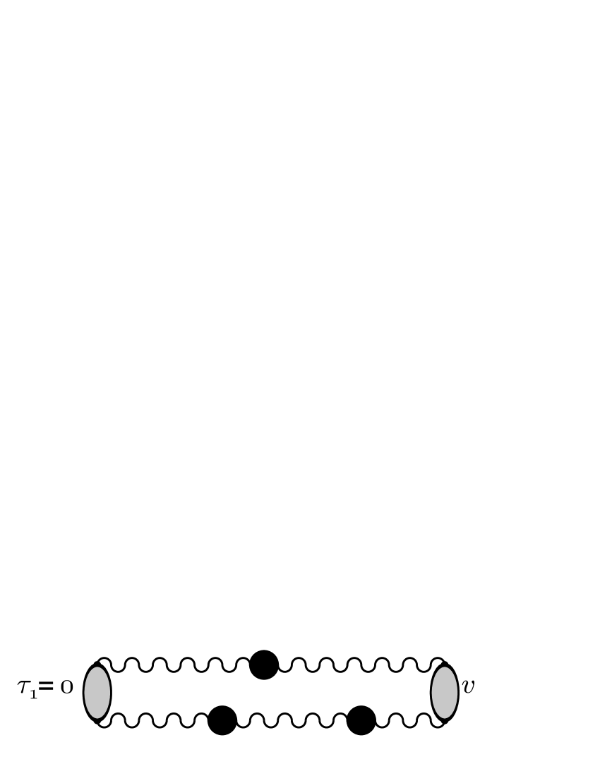
FIG. 1.: A diagram that contributes to $f(\tau)$ after it is integrated with respect to $v$, which denotes the most distant point to the right. The wavy lines represent the logarithmic Coulomb interaction between the charged particles of the gas. The black dots are the polarization operators of the gas inside the interval $(0,v)$, while the shaded bubbles are related to the polarization of the gas near the ending points $0$ and $v$.

REFERENCES

- [1] Also at the Landau Institute for Theoretical Physics, Russia.
- [2] J. M. Calleja et al., Solid State Commun. 79, 911 (1991).
- [3] T. Ogawa, A. Furusaki, and N. Nagaosa, Phys. Rev. Lett. 68, 3638 (1992).
- [4] D. K. K. Lee and Y. Chen, Phys. Rev. Lett. 69, 1399 (1992).
- [5] A. O. Gogolin, Phys. Rev. Lett. 71, 2995 (1993).
- [6] N. V. Prokof’ev, Phys. Rev. B 49, 2148 (1994).
- [7] C. L. Kane, K. A. Matveev, and L. I. Glazman, Phys. Rev. B 49, 2253 (1994).
- [8] I. Affleck and W. W. Ludwig, J. Phys. A: Math and Gen. 27, 5375 (1994).
- [9] G. D. Mahan, Phys. Rev. 163, 612 (1967).
- [10] P. W. Anderson, Phys. Rev. Lett. 18, 1049 (1967).
- [11] G. Yuval and P. W. Anderson, Phys. Rev. B 1, 1522 (1970).
- [12] B. Roulet, J. Gavoret, and P. Noziéres, Phys. Rev. 178, 1072 (1969).
- [13] P. Noziéres, J. Gavoret, and B. Roulet, Phys. Rev. 178, 1084 (1969).
- [14] P. Noziéres and C. T. De Dominicis, Phys. Rev. 178, 1097 (1969).
- [15] D. C. Mattis and E. H. Lieb, J. Math. Phys. 6, 304 (1965).
- [16] I. E. Dzyaloshinskii and A. I. Larkin, Zh. Eksp. Teor. Fiz 65, 411 (1973), [Sov. Phys. 38 202 (1974)].
- [17] A. Luther and I. Peschel, Phys. Rev. B 9, 2911 (1974).
- [18] K. D. Schotte and U. Schotte, Phys. Rev. 182, 479 (1969).
- [19] P. W. Anderson, G. Yuval, and D. R. Hamman, Phys. Rev. B 1, 4464 (1970).
- [20] K. D. Schotte, Z. Physik 230, 99 (1970).
- [21] C. L. Kane and M. P. A. Fisher, Phys. Rev. Lett. 68, 1220 (1992).
- [22] C. L. Kane and M. P. A. Fisher, Phys. Rev. B 46, 15233 (1992).
- [23] J. Sólyom, Adv. Phys. 28, 201 (1979).
- [24] E. Fradkin, in Field Theories of Condensed Matter Systems, Frontiers in Physics (Addison–Wesley, Redwood City, CA, 1991), Chap. 4.
- [25] S. T. Chui and P. A. Lee, Phys. Rev. Lett. 35, 315 (1975).
- [26] A. J. Leggett et al., Rev. Mod. Phys. 59, 1 (1987).
- [27] J. V. Jose, L. P. Kadanoff, S. Kirkpatrick, and D. R. Nelson, Phys. Rev. B 16, 1217 (1977).
- [28] L. P. Kadanoff, J. Phys. A: Math and Gen. 11, 1399 (1978).
- [29] J. M. Kosterlitz, J. Phys. C 7, 1046 (1974).
- [30] J. M. Kosterlitz and D. J. Thouless, J. Phys. C 6, 1181 (1973).
- [31] S. A. Bulgadaev, Teor. Matem. Fiz. 51, 424 (1982), phys. Lett. A 86, 213 (1981).
- [32] This is in agreement with the well known result for the energy levels correlation function of random matrices (M. L. Metha, Random Matrices (Academic Press, Inc., Boston, 1990).). As was shown by Dyson (F. J. Dyson, J. Math. Phys. 3, 140 (1962)) there is a direct correspondence between the statistics of energy levels of complex systems and the statistical mechanics of a logarithmic Coulomb gas.
- [33] V. J. Emery, in Highly Conducting One-Dimensional Solids, edited by J. T. Devreese, R. P. Evrard, and V. E. van Doren (Plenum, New York, 1979), p. 327.
- [34] R. Floreanini and R. Jackiw, Phys. Rev. Lett. 59, 1873 (1987).
- [35] K. G. Wilson and J. B. Kogut, Physics Reports C 12, 75 (1974).
- [36] H. Lipkin, Quantum Mechanics: New approaches to selected topics (North–Holland, Amsterdam, 1973).
- [37] J. Friedel, Philos. Mag. 43, 153 (1952).
- [38] J. Friedel, Nuovo Cimento Suppl. 87, 287 (1958).
- [39] J. S. Langer and V. Ambegaokar, Phys. Rev. 121, 1090 (1961).
- [40] F. Guinea, Phys. Rev. B 32, 7518 (1985).
- [41] K. A. Matveev, Phys. Rev. B 51, 1743 (1995).
- [42] V. J. Emery and S. Kivelson, Phys. Rev. B 46, 10812 (1992).