NMR and Neutron Scattering Experiments on the Cuprate Superconductors: A Critical Re-Examination

Abstract

We show that it is possible to reconcile NMR and neutron scattering experiments on both $\rm La_{2-x}Sr_{x}CuO_{4}$ and $\rm YBa_{2}Cu_{3}O_{6+x}$, by making use of the Millis-Monien-Pines mean field phenomenological expression for the dynamic spin-spin response function, and reexamining the standard Shastry-Mila-Rice hyperfine Hamiltonian for NMR experiments. The recent neutron scattering results of Aeppli $et~{}al$[1] on $\rm La_{1.86}Sr_{0.14}CuO_{4}$ are shown to agree quantitatively with the NMR measurements of ${}^{63}T_{1}$ and the magnetic scaling behavior proposed by Barzykin and Pines.[2] The reconciliation of the $\rm{}^{17}O$ relaxation rates with the degree of incommensuration in the spin fluctuation spectrum seen in neutron experiments is achieved by introducing a new transferred hyperfine coupling $C^{\prime}$ between $\rm{}^{17}O$ nuclei and their next nearest neighbor $Cu^{2+}$ spins; this leads to a near-perfect cancellation of the influence of the incommensurate spin fluctuation peaks on the $\rm{}^{17}O$ relaxation rates of $\rm La_{2-x}Sr_{x}CuO_{4}$. The inclusion of the new $C^{\prime}$ term also leads to a natural explanation, within the one-component model, the different temperature dependence of the anisotropic $\rm{}^{17}O$ relaxation rates for different field orientations, recently observed by Martindale $et~{}al$.[3] The measured significant decrease with doping of the anisotropy ratio, ${}^{63}R=^{63}T_{1ab}/^{63}T_{1c}$ in $\rm La_{2-x}Sr_{x}CuO_{4}$ system, from ${}^{63}R=3.9$ for ${\rm La_{2}CuO_{4}}$ to ${}^{63}R\simeq 3.0$ for $\rm La_{1.85}Sr_{0.15}CuO_{4}$ is made compatible with the doping dependence of the shift in the incommensurate spin fluctuation peaks measured in neutron experiments, by suitable choices of the direct and transferred hyperfine coupling constants $A_{\beta}$ and B.

I introduction

The magnetic behavior of the planar excitations in the cuprate superconductors continues to be of central concern to the high temperature superconductivity community. Not only does it provide significant constraints on candidate theoretical descriptions of their anomalous normal state behavior, but it may also hold the key to the physical origin of high temperature superconductivity. Recently two of us have used the results of NMR experiments to determine the magnetic phase diagram for the $La_{2-x}Sr_{x}CuO_{4}$ and $YBa_{2}Cu_{3}O_{6+x}$ systems.[2] We found that for both systems bulk properties, such as the spin susceptibility, and probes in the vicinity of the commensurate antiferromagnetic wave vector ($\pi,\pi$), such as ${}^{63}T_{1}$, the ${}^{63}Cu$ spin relaxation time, and ${}^{63}T_{2G}$, the spin-echo decay time, display $z=1$ scaling and spin pseudogap behavior over a wide regime of temperatures. On the other hand, the neutron scattering experimental results of Aeppli et al[1] on $La_{1.86}Sr_{0.14}CuO_{4}$ which probe directly $\chi^{\prime\prime}(q,\omega)$, the imaginary part of the spin-spin response function, while supporting this proposed scaling behavior, at first sight appear incapable of explaining NMR experiments on this system.

This apparent contradiction between the results of NMR and neutron scattering experiments, both of which probe $\chi(q,\omega)$ in $La_{1.86}Sr_{0.14}CuO_{4}$, is but one of a series of such apparent contradictions. For example, in the $YBa_{2}Cu_{3}O_{6+x}$ system, NMR experiments on ${}^{63}Cu$ and ${}^{17}O$ nuclei in both $YBa_{2}Cu_{3}O_{7}$[4] and $YBa_{2}Cu_{3}O_{6.63}$[5] require the presence of strong antiferromagnetic correlations between the planar $Cu^{2+}$ spins, and a simple mean field description of the spin-spin response function with a temperature dependent magnetic correlation length $\xi\gtrsim 2$, was shown to provide a quantitative description of the measured results for ${}^{63}T$ and ${}^{17}T_{1}$ in $YBa_{2}Cu_{3}O_{7}$,[6] and $YBa_{2}Cu_{3}O_{6.63}$.[7] Yet neutron scattering experiments on $YBa_{2}Cu_{3}O_{7}$[8, 9, 10] and $YBa_{2}Cu_{3}O_{6.63}$,[11] find only comparatively broad, temperature-independent, peaks in $\chi^{\prime\prime}(q,\omega)$, corresponding to a quite short ($\xi\lesssim 1$) temperature-independent magnetic correlation length. The apparent contradiction is especially severe for the $\rm La_{2-x}Sr_{x}CuO_{4}$ system, where neutron scattering experiments show at low temperatures four incommensurate peaks in the spin fluctuation spectrum, whose position depends on the level of Sr doping,[12] while the quantitative explanation (using the same one-component phenomenological description which worked for the $\rm YBa_{2}Cu_{3}O_{6+x}$ system) of the measurements of ${}^{63}T_{1}$ and ${}^{17}T_{1}$ in this system requires that the spin fluctuations be peaked at ($\pi,\pi$), or nearly so.[13, 14] Viewed from the NMR perspective, there are two major problems with four incommensurate spin fluctuation peaks. First, the Shastry-Mila-Rice (SMR) form factor,[15, 16] which, provided the peaks are nearly at ($\pi,\pi$), effectively screens neighboring ${}^{17}O$ nuclei from the presence of the strong peaks in the nearly localized $Cu^{2+}$ spin spectrum required to explain the anomalous temperature-dependence behavior of ${}^{63}T_{1}$, fails to do so for the considerable degree of incommensuration in the peaks at ($\pi,[\pi\pm\delta])$ and $([\pi\pm\delta],\pi$) seen in $La_{1.86}Sr_{0.14}CuO_{4}$.[14, 17, 18] As a result ${}^{17}T_{1}$ picks up a substantial anomalous temperature dependence which is not seen experimentally. Second, with the doping-independent values of the hyperfine couplings which appear in the SMR form factors for a commensurate spectrum, the calculated anisotropy of ${}^{63}T_{1}$ for the incommensurate peaks seen by neutrons is in sharp variance with what is seen in the NMR experiments.[14]

Two ways out of these apparent contradictions have been proposed. One view is that the spin fluctuation peaks seen in the neutron scattering experiments reflect the appearance of discommensuration, not incommensuration; on this view, the $\rm La_{2-x}Sr_{x}CuO_{4}$ system contains domains in which the spin fluctuation peaks are commensurate (so that there are no problems with ${}^{17}T_{1}$), but what neutrons, a global probe, see is the periodic array of the domain walls.[19] A second view is that a one-component description of $\chi({\bf q},\omega)$ is not feasible; rather, the transferred hyperfine coupling between the nearly localized $Cu^{2+}$ spins and the ${}^{17}O$ nuclei is presumed to be very weak, and the ${}^{17}O$ nuclei are assumed to be relaxed by a different mechanism, whence the nearly Korringa-like behavior of ${}^{17}T_{1}$.[18] A further challenge to a one-component description has come from the very recent work of Martindale et al,[3] who find that their results for the temperature-dependence of the planar anisotropy of ${}^{17}T_{1\alpha}$ for different field orientations appear incompatible with a one-component description.

In the present paper we present a third view: that the one-component phenomenological description is valid, but what requires modification are the hyperfine couplings which appear in the SMR Hamiltonian which describes planar nuclei coupled to nearly localized $Cu^{2+}$ spins. We find that by introducing a transferred hyperfine coupling $C^{\prime}$, between the next nearest neighbor $Cu^{2+}$ spins and a ${}^{17}O$ nucleus, the nearly antiferromagnetic part of the strong signals emanating from the $Cu^{2+}$ spins can be far more effectively screened than is possible with only a nearest neighbor transferred hyperfine coupling, so that the existence of four incommensurate peaks in the $\rm La_{2-x}Sr_{x}CuO_{4}$ system can be made compatible with the ${}^{17}T_{1}$ results. We also find that by permitting the transferred hyperfine coupling, $B$, between a $Cu^{2+}$ spin and its nearest neighbor ${}^{63}Cu$ nucleus to vary with doping, we can explain the trend with doping of the anisotropy of ${}^{63}T_{1}$ in this system. We then use these revised hyperfine couplings to reexamine the extent to which the recent results of Aeppli et al[1] on $\rm La_{1.86}Sr_{0.14}CuO_{4}$ can be explained quantitatively by combining the Millis-Monien-Pines (hereafter MMP) response function[6] with the scaling arguments put forth by Barzykin and Pines.[2] We find that they can, and are thus able to reconcile the neutron scattering and NMR experiments on this member of the $\rm La_{2-x}Sr_{x}CuO_{4}$ system.

We present as well the results of a reexamination of the NMR and neutron results for the $\rm YBa_{2}Cu_{3}O_{6+x}$ system. Here we begin by making the ansatz that it is the presence of incompletely resolved incommensurate peaks which is responsible for the broad lines seen in neutron experiments. We follow Dai et al,[9] who suggest the increased line width for $\rm YBa_{2}Cu_{3}O_{7}$ seen along the zone diagonal directions reflects the presence of four incommensurate peaks, located at ${\bf Q}_{i}=(\pi\pm\delta,\pi\pm\delta)$, a proposal which is consistent with the earlier measurements of Tranquada $et~{}al$ for $YBa_{2}Cu_{3}O_{6.6}$ [11]. We then find that incommensuration can be made compatible with NMR experimental results provided the transferred hyperfine coupling constant, $B$, is doping dependent in this system as well. Moreover, on considering ${}^{17}T_{1}$ for $\rm YBa_{2}Cu_{3}O_{7}$, we find that the anomalous temperature dependence of the planar anisotropy of ${}^{17}T_{1}$ measured by Martindale $et~{}al$[3] constitutes a proof of the validity of our modified one-component model. Thus incommensuration combined with the presence of the next nearest neighbor coupling, $C^{\prime}$, leads to results which are consistent with experiment, and we are able to preserve the one-component description of the planar spin excitation spectrum.

The outline of our paper is as follows: In Section II we review the SMR description of coupled $Cu^{2+}$ spins and nuclei as well as the mean field description of $\chi({\bf q},\omega)$, and examine the modifications brought about by incommensuration and next nearest neighbor coupling between $Cu^{2+}$ spins and a ${}^{17}O$ nucleus. In Section III we review the experimental constraints on the hyperfine coupling parameters, and present our results for their variation with doping in both the $\rm La_{2-x}Sr_{x}CuO_{4}$ and $\rm YBa_{2}Cu_{3}O_{6+x}$ systems. We show in Section IV how the ${}^{63}Cu$ NMR results can be reconciled with neutron scattering results on $\rm La_{1.86}Sr_{0.14}CuO_{4}$, while in Section V we present a quantitative fit to the ${}^{17}T_{1c}$ results for the $La_{1.85}Sr_{0.15}CuO_{4}$ based on the four incommensurate peaks in the spin fluctuation spectrum expected from neutron scattering. We show in Section VI how the anomalous results of Martindale et al[3] for the $\rm YBa_{2}Cu_{3}O_{6+x}$ system can be explained using our modified one-component model, and in Section VII we present our conclusions.

II A Generalized Shastry-Mila-Rice Hamiltonian

On introducing a hyperfine coupling $C^{\prime}_{\alpha,\beta}$ between the the ¹⁷O nuclei and their next nearest neighbor $Cu^{2+}$ spins, we can rewrite the SMR hyperfine Hamiltonian for the $\rm{}^{63}Cu$ and $\rm{}^{17}O$ nuclei as:

$$H_{hf}= {}^{63}I_{\alpha}({\bf r}_{i})\Big{[}\sum_{\beta}A_{\alpha,\beta}S_{\beta}({\bf r}_{i})+B\sum_{j}^{nn}S_{\alpha}({\bf r}_{j})\Big{]}$$ (1)

$$+ {}^{17}I_{\alpha}({\bf r}_{i})\Big{[}C_{\alpha,\beta}\sum_{j,\beta}^{nn}S_{\beta}({\bf r}_{j})+C^{\prime}_{\alpha,\beta}\sum_{j,\beta}^{nnn}S_{\beta}({\bf r}_{j})\Big{]}$$ (2)

where $A_{\alpha,\beta}$ is the tensor for the direct, on-site coupling of the ${\rm{}^{63}Cu}$ nuclei to the Cu²⁺ spins, $B$ is the strength of the transferred hyperfine coupling of the ${\rm{}^{63}Cu}$ nuclear spin to the four nearest neighbor Cu²⁺ spins, $C_{\alpha,\beta}$ is the transferred hyperfine coupling of the $\rm{}^{17}O$ nuclear spin to its nearest neighbor Cu²⁺ spins, and $C^{\prime}_{\alpha,\beta}$ its coupling to the next nearest neighbor Cu²⁺ spins. The indices “$nn$” represent nearest neighbor electron spins to the specific nuclei, “$nnn$” the next nearest neighbor $Cu^{2+}$ spins. As we shall see below, inclusion of the $C^{\prime}_{\alpha,\beta}$ term enhances the cancellation of the anomalous antiferromagnetic spin fluctuations seen by the $\rm{}^{17}O$ nucleus, and therefore reduces the leakage from incommensurate spin fluctuation peaks to the $\rm{}^{17}O$ relaxation rates. It thus enable us to reconcile the measured $\rm{}^{17}O$ relaxation rates with the neutron scattering experiments for both $\rm La_{2-x}Sr_{x}CuO_{4}$ and $\rm YBa_{2}Cu_{3}O_{6+x}$.

The spin contribution to the NMR Knight shift for the various nuclei are:[6]

$${}^{63}K_{c} = \frac{(A_{c}+4B)\chi_{0}}{{}^{63}\gamma_{n}\gamma_{e}\hbar^{2}}$$ (3)

$${}^{63}K_{ab} = \frac{(A_{ab}+4B)\chi_{0}}{{}^{63}\gamma_{n}\gamma_{e}\hbar^{2}}$$ (4)

$${}^{17}K_{\beta} = \frac{2(C_{\beta}+2C^{\prime}_{\beta})\chi_{0}}{{}^{17}\gamma_{n}\gamma_{e}\hbar^{2}}$$ (5)

Here, we have incorporated the new $C^{\prime}_{\beta}$ term into the $\rm{}^{17}O$ Knight shift expression for ${}^{17}K_{\beta}$, while the others remain their standard form as in Ref.[6], $\gamma_{n}$ are various nuclei gyromagnetic ratios, $\gamma_{e}$ is the electron gyromagnetic ratio, and $\chi_{0}$ the static spin susceptibility. The indices $c$ and $ab$ refer to the direction of the applied static magnetic field along the $c$-axis and the $ab$-plane. The spin-lattice relaxation rate, $(^{\alpha}T_{1})^{-1}_{\beta}$, for nuclei $\alpha$ responding to a magnetic field in the $\beta$ direction, is:

$${}^{\alpha}T^{-1}_{1\beta}=\frac{k_{B}T}{2\mu_{B}^{2}\hbar^{2}\omega}\sum_{{\bf q}}{{}^{\alpha}F_{\beta}({\bf q})}\chi^{\prime\prime}({\bf q},\omega\rightarrow 0)$$ (6)

where the modified SMR form factors, ${}^{\alpha}F_{\beta}({\bf q})$, are now given by:

$${}^{63}F_{c} = [A_{ab}+2B(\cos q_{x}a+\cos q_{y}a)]^{2}$$ (7)

$${}^{63}F_{ab} = \frac{1}{2}[~{}^{63}F_{c}+^{63}F_{ab}^{eff}]$$ (8)

$${}^{63}F_{ab}^{eff} = [A_{c}+2B(\cos q_{x}a+\cos q_{y}a)]^{2}$$ (9)

$${}^{17}F_{\alpha} = 2\sum_{\alpha_{i}=\alpha^{\prime},\alpha^{\prime\prime}}\cos^{2}\frac{q_{x}a}{2}\big{(}C_{\alpha_{i}}+2C^{\prime}_{\alpha_{i}}\cos q_{y}a\big{)}^{2},$$ (10)

Here, $\alpha^{\prime}$ and $\alpha^{\prime\prime}$ are the directions perpendicular to $\alpha$. The form factor ${}^{63}F_{ab}^{eff}$ is the filter for the ${\rm{}^{63}Cu}$ spin-echo decay time ${}^{63}T_{2G}$[20]:

$${}^{63}T_{2G}^{-2}=\frac{.69}{128\hbar^{2}\mu_{B}^{4}}\left\{\frac{1}{N}\,\sum_{\bf q}F_{ab}^{eff}({\bf q})^{2}[\chi^{\prime}({\bf q},0)]^{2}-\left[\frac{1}{N}\sum_{\bf q}F_{ab}^{eff}({\bf q})\chi^{\prime}({\bf q},0)\right]^{2}\right\}$$ (11)

The values of the hyperfine constant $C_{\alpha}$ and $C^{\prime}_{\alpha}$ can be determined by the various $\rm{}^{17}O$ Knight shift data. In fact, we may obtain these new values from the “old” values of the hyperfine coupling constant, $C_{\alpha}^{\rm old}$, which have been well established from fitting the Knight shift data.[2] Note we use $C_{\alpha}$ to represent the new nearest neighbor hyperfine coupling constant, while the old hyperfine coupling constant is written explicitly as $C_{\alpha}^{\rm old}$ throughout the paper. In order not to change the Knight shift result of the previous analysis[2], the new hyperfine coupling constants should satisfy the following requirement:

$$C_{\alpha}+2C^{\prime}_{\alpha}=C^{\rm old}_{\alpha}=\zeta_{\alpha}C_{c}^{\rm old}$$ (12)

where $\zeta_{\alpha}=C_{\alpha}^{\rm old}/C_{c}^{\rm old}$, and $c$ denotes the case of a magnetic field along the $c$-axis. For $\rm YBa_{2}Cu_{3}O_{6+x}$, from the previous analysis of Yoshinari[21] and Martindale $et~{}al$[3], we have for a field parallel to the Cu-O bond, $\zeta_{\parallel}$=1.42, and $\zeta_{\perp}=0.91$ for a field perpendicular to the Cu-O bond direction, while $\zeta_{c}=1$. On introducing $r_{\alpha}\equiv C^{\prime}_{\alpha}/C_{c}$ we obtain:

$$C_{\alpha} = C_{c}^{\rm old}(\zeta_{\alpha}-\frac{2r_{\alpha}}{2r_{c}+1})$$ (13)

$$C^{\prime}_{\alpha} = C_{c}^{\rm old}\frac{r_{\alpha}}{2r_{c}+1}$$ (14)

Substituting these values of $C_{\alpha}$ and $C^{\prime}_{\alpha}$ into Eq.(10), we obtain the new $\rm{}^{17}O$ form factor in terms of $C^{\rm old}_{\alpha}$:

$${}^{17}F_{\alpha}=\frac{2(C_{c}^{\rm old})^{2}}{(1+2r_{c})^{2}}\sum_{\alpha_{i}=\alpha^{\prime},\alpha^{\prime\prime}}\cos^{2}\frac{q_{x}a}{2}[\zeta_{\alpha_{i}}(1+2r_{c})-2r_{\alpha_{i}}+2r_{\alpha_{i}}\cos q_{y}a]^{2}$$ (15)

Although $C^{\prime}_{\alpha}$ may well be anisotropic (as $C_{\alpha}$ is), in the absence of detailed quantum chemistry calculations, (which lie beyond the purview of the present paper) we assume $C^{\prime}_{\alpha}$ to be isotropic for illustrative purposes, in which case $r_{\perp}=r_{\parallel}=r_{c}\equiv r\equiv C^{\prime}/C_{c}$. In Fig.1, we compare our modified form factor ${}^{17}F_{c}$, Eq(15), with the standard SMR form. It is seen that with a comparatively small amount of next nearest neighbor coupling, corresponding to $r\equiv C^{\prime}/C_{c}=0.25$, the new form factor is reduced significantly near $(\pi/a,\pi/a)$, and is some 30% narrower near ${\bf q}=0$. This indicates that the oxygen $(^{17}T_{1}T)^{-1}$ is less likely to pick up the anomalous antiferromagnetic contribution near $(\pi/a,\pi/a)$, even when the anomalous spin fluctuation is slightly spread away from $(\pi/a,\pi/a)$.

We adopt the phenomenological MMP expression for the spin-spin correlation function, modified to take into account the presence of four incommensurate peaks at ${\bf Q}_{i}$ near $(\pi/a,\pi/a)$[2],

$$\chi({\bf q},\omega)=\frac{1}{4}\sum_{i}\frac{\alpha\xi^{2}\mu_{B}^{2}}{1+({\bf q}-{\bf Q}_{i})^{2}\xi^{2}-i\omega/\omega_{SF}}+\frac{{\chi}_{0}(T)}{1-i\pi\omega/\Gamma}$$ (16)

Here the first term, often called $\chi_{AF}$, represents the anomalous contribution to the spin spectrum, brought about by the close approach to antiferromagnetism of the Fermi liquid in the vicinity of the peaks at ${\bf q}={\bf Q}_{i}$ determined by neutron scattering experiments[1, 23]. For $\rm La_{1.86}Sr_{0.14}CuO_{4}$, ${\bf Q}_{i}=(\pi/a,[\pi\pm\delta]/a),([\pi\pm\delta]/a,\pi/a)$, with $\delta=0.245\pi$. In Eq.(16), $\omega_{SF}$ is the characteristic frequency of the spin fluctuations, $\xi$ is the correlation length, and $\alpha$ is the scale factor (in units of states/eV, where $\mu_{B}$ is the Bohr magneton), which relates $\chi_{{\bf Q}_{i}}$ to $\xi^{2}$; thus the height of each of the four peaks is,

$$\chi_{{\bf Q}_{i}}=\frac{\alpha}{4}\xi^{2}\mu_{B}^{2}.$$ (17)

The second term on the right-hand side of Eq.(16), usually called $\chi_{FL}$, is a parameterized form of the normal Fermi Liquid contribution, which is wave-vector independent over most of the Brillouin zone; $\Gamma$ is of order the Fermi energy. The static bulk susceptibility $\chi_{0}$, which is generally temperature dependent, has been determined for $\rm La_{2-x}Sr_{x}CuO_{4}$ and $\rm YBa_{2}Cu_{3}O_{6+x}$ from copper and oxygen Knight shift experiments.[2] For a system with any appreciable antiferromagnetic correlations ($\xi\gtrsim a$), the normal Fermi liquid contribution is small compared to $\chi_{AF}$ for wave vectors in the vicinity of ${\bf Q}_{i}$, and plays a negligible role in determining $(^{63}T_{1}T_{c})^{-1}$; however, because of the filtering action of ${}^{17}F_{\alpha}$, it makes a significant contribution to $(^{17}T_{1}T)^{-1}$. Note that because the MMP expression for $\chi_{AF}$ is a good approximation only for wave vectors in the vicinity of the antiferromagnetic wave vector ${\bf Q}_{i}$, the above expression should not be used in calculating long wavelength properties, such as the Knight shift of $\rm{}^{17}O$.

For the frequently encountered case of long correlation lengths ($\xi\gtrsim 2a$), in calculating the various $\rm{}^{63}Cu$ relaxation rates one can approximate $\chi^{\prime\prime}({\bf q},\omega)$ by $\chi^{\prime\prime}({\bf Q}_{i},\omega)\delta({\bf q}-{\bf Q}_{i})$. One can then replace Eq.(6) and (11) by the following analytic expressions:

$$\frac{1}{{}^{63}T_{1\beta}T} \simeq \frac{k_{B}}{8\pi\hbar}{{}^{63}F_{\beta}}({\bf Q}_{i})\frac{\alpha}{\hbar\omega_{SF}}$$ (18)

$$(1/^{63}T_{2G})^{2} \simeq \frac{.69}{512}\frac{{}^{63}F_{ab}^{eff}({\bf Q}_{i})^{2}\alpha^{2}\xi^{2}}{\pi\hbar^{2}}.$$ (19)

Another important quantity, the anisotropy ratio of the $\rm{}^{63}Cu$ spin-lattice relaxation rates, which has been measured for $\rm La_{2-x}Sr_{x}CuO_{4}$ and $\rm YBa_{2}Cu_{3}O_{6+x}$ at various doping concentrations, provides a direct constraint on the hyperfine coupling constants, $A_{\alpha}$ and $B$. For $\xi\gtrsim 2$, this anisotropy ratio, ${}^{63}R$ can be written as,

$${}^{63}R\equiv\frac{T_{1c}}{T_{1ab}}\simeq\frac{{}^{63}F_{ab}({\bf Q}_{i})}{{}^{63}F_{c}({\bf Q}_{i})}.$$ (20)

For the case of $\rm La_{2-x}Sr_{x}CuO_{4}$, where the peaks are located at ${\bf Q}_{i}=(\pi/a,[\pi\pm\delta]/a),([\pi\pm\delta]/a,\pi/a)$, we then have

$${}^{63}R\simeq\frac{1}{2}\left[1+\frac{\Big{(}A_{c}-2B(1+\cos\delta)\Big{)}^{2}}{\Big{(}A_{ab}-2B(1+\cos\delta)\Big{)}^{2}}\right].$$ (21)

For $\rm YBa_{2}Cu_{3}O_{6+x}$, as indicated in the Introduction, on assuming the broad $(\pi/a,\pi/a)$ peak seen in neutron scattering experiments[8, 9, 10, 11] reflects the presence of four unresolved overlapping incommensurate peaks located along the zone diagonal directions,[9, 11] we may write

$${\bf Q}_{i}=([\pi\pm\delta]/a,[\pi\pm\delta]/a),$$ (22)

and the anisotropy ratio becomes,

$${}^{63}R\simeq\frac{1}{2}\left[1+\frac{(A_{c}-4B\cos\delta)^{2}}{(A_{ab}-4B\cos\delta)^{2}}\right].$$ (23)

Numerical calculations of the $\rm{}^{17}O$ relaxation rates show that these rates can deviate significantly from those obtained by approximating the $\chi_{AF}^{\prime\prime}$ by a $\delta({\bf q}-{\bf Q}_{i})$ function. We therefore calculate the $\rm{}^{17}O$ relaxation rates numerically, using Eqs.(6) and (10).

III The Direct and Transferred Hyperfine Constants

Seven years of NMR experiments on aligned powders and single crystals of the cuprates have produced a significant number of constraints which must be taken into account in selecting the hyperfine constants which enter the SMR Hamiltonian. Thus experiments which determine the $\rm{}^{63}Cu$ nuclear resonance frequency in the $AF$ insulators, $YBa_{2}Cu_{3}O_{6}$[24] and $La_{2}CuO_{4}$[25], yield similar results for the product of $(4B-A_{ab})$ and $\mu_{eff}$, the effective moment of the localized Cu²⁺ spins,[26]

$$\mu_{eff}(4B-A_{ab}) = 79.65\pm 0.05~{}~{}kOe\hskip 43.36243pt\mbox{(YBa${}_{2}$Cu${}_{3}$O${}_{6}$)}$$ (24)

$$\mu_{eff}(4B-A_{ab}) = 78.78~{}~{}kOe\hskip 86.72377pt\mbox{(La${}_{2}$CuO${}_{4}$)}$$ (25)

On using the value, $\mu_{eff}=0.62\mu_{B}$, determined by Manousakis[27] for the 2D spin $1/2$ Heisenberg antiferromagnet, we then find

$$4B-A_{ab} = 128.5~{}~{}kOe/\mu_{B}\hskip 86.72377pt(\rm{YBa_{2}Cu_{3}O_{6}})$$ (26)

$$4B-A_{ab} = 127~{}~{}kOe/\mu_{B}\hskip 86.72377pt(\rm{La_{2}CuO_{4}})$$ (27)

A second set of constraints comes from ${}^{63}Cu$ Knight shift experiments. To a high degree of accuracy, in the $\rm YBa_{2}Cu_{3}O_{6+x}$ system the $\rm{}^{63}Cu$ Knight shift in a magnetic field along the $c$-axis is temperature independent in both the normal and superconducting state, and hence reflects only the chemical shift. The absence of a spin contribution means that for this system,

$$A_{c}+4B\simeq 0,$$ (28)

independent of doping level. A third set of constraints is obtained from measurements of the anisotropy of the ${}^{63}Cu$ spin-lattice relaxation rates; for $YBa_{2}Cu_{3}O_{7}$ one finds ${}^{63}R=3.7\pm 0.1$.[28] To the extent that $A_{ab}$, $A_{c}$, and $B$ are independent of doping level in $\rm YBa_{2}Cu_{3}O_{6+x}$, and the spin fluctuation peaks are commensurate (or nearly so) for this system, one then finds from Eqs. (23), (26), and (28), that

$$B = 40.8~{}~{}kOe/\mu_{B}$$ (29)

$$A_{c} = -163~{}~{}kOe/\mu_{B}$$ (30)

$$A_{ab} = 34~{}~{}kOe/\mu_{B}$$ (31)

in agreement with the analysis of Monien, Pines, and Takigawa.[7] These values are consistent with the constraint on $(4B+A_{ab})$ obtained by Ishida et al for $La_{1.85}Sr_{0.15}CuO_{4}$; from the slope of a plot of their direct measurement of $\chi_{o}(T)$ against their measured value of ${}^{63}K_{ab}(T)$, they found[29]

$$4B+A_{ab}=189~{}~{}kOe/\mu_{B}.$$ (32)

It seemed natural therefore to conclude that not only were $A_{ab}$, $A_{c}$, and $B$ independent of doping for the $\rm YBa_{2}Cu_{3}O_{6+x}$ system, but that the corresponding values for the $\rm La_{2-x}Sr_{x}CuO_{4}$ system were likewise doping independent and were virtually identical with those deduced for $\rm YBa_{2}Cu_{3}O_{6+x}$.

If, however, the spin fluctuation peaks in the $\rm La_{2-x}Sr_{x}CuO_{4}$ system are incommensurate, the assumption that the hyperfine constraints for this system are doping independent is no longer tenable for this system, as may be seen by comparing the measured values of ${}^{63}R$ for the $\rm La_{2-x}Sr_{x}CuO_{4}$ system shown in Table I with the values calculated using Eqs(31), and using the doping dependence of the degree of incommensuration determined in neutron scattering experiments[12], $\delta\sim 1.75x$, where $x$ is the $Sr$ doping level. As may be seen in Table I, the calculated trend with doping is opposite to that seen experimentally. Since the quantum chemical environment responsible for the direct hyperfine interaction $A_{\alpha}$ is not expected to vary substantially with doping, the most likely culprit in Eqs.(31) is the assumption that the transferred hyperfine coupling constant does not vary appreciably with doping; indeed, if $B$ increases sufficiently rapidly with doping, with $A_{ab}$ and $A_{c}$ fixed, one can find a doping dependence of ${}^{63}R$ which is more nearly in accord with experiment. This means abandoning for the $\rm La_{2-x}Sr_{x}CuO_{4}$ system the constraint, $A_{c}\simeq-4B$, which works so well for the $\rm YBa_{2}Cu_{3}O_{6+x}$ system.

Suppose then one starts anew with the insulator, $La_{2}CuO_{4}$. On making use of Eqs. (21) and (32) and taking ${}^{63}R=3.9$, in accord with the result of Imai $et~{}al$[30] at $475$K, one finds readily that

$$A_{ab}-A_{c}=203~{}~{}kOe/\mu_{B}.$$ (33)

On turning next to $La_{1.85}Sr_{0.15}CuO_{4}$, taking ${}^{63}R=3.0$, in accord with the recent measurement of Milling and Slichter,[31] using the result of Ishida et al,[29] Eq.(32), and assuming that $A_{\alpha\beta}$ is independent of doping, one then finds $B=48~{}kOe/\mu_{B}$ and $A_{ab}=-3~{}kOe/\mu_{B}$. This result is, however, unrealistic. A straightforward calculation using the expressions adapted by Monien et al[26] from the work of Bleaney et al[32],

$$A_{c} = 395[{-\hat{\kappa}-{4\over 7}-{62\over 7}\gamma}]~{}~{}kOe/\mu_{B}$$ (34)

$$A_{ab} = 395[{-\hat{\kappa}-{2\over 7}-{11\over 7}\gamma}]~{}~{}kOe/\mu_{B}$$ (35)

In Eqs.(35), $\gamma\equiv\lambda/E_{xy}$ is the dimensionless ratio of the spin-orbit coupling for a Cu²⁺ ion, $\lambda\sim-710cm^{-1}$, to the excitation energy from the ground state of the $\rm{}^{63}Cu$ $d_{x^{2}-y^{2}}$ orbital of the various $\rm{}^{63}Cu$ $d$ states, $E_{xy}\sim E_{xz}\sim E_{yz}\sim 2eV$; with these typical values, $\gamma=0.044\pm 0.009$; $\langle{1\over r^{3}}\rangle$ which enters as a multiplicative factor in Eq. (35) is taken to be $6.3a^{-3}_{o}$. With the value of $\gamma=0.0469$ obtained using Eq. (33),

$$A_{ab}=(-395\hat{\kappa}+142)~{}~{}kOe/\mu_{B}.$$ (36)

On taking the core polarization $\hat{\kappa}=0.26\pm 0.06$[26], we then get, for $\hat{\kappa}$ in the vicinity of its plausible upper limit, 0.32,

$$A_{ab}\geq 16~{}~{}kOe/\mu_{B}.$$ (37)

In order to satisfy the above constraints, we next assume that the anisotropy, ${}^{63}R$, for $\rm La_{1.85}Sr_{0.15}CuO_{4}$ is at the upper end of the range quoted by Milling and Slichter, and take ${}^{63}R=3.2$; we next take $A_{ab}=18~{}kOe/\mu_{B}$ (corresponding to $\hat{\kappa}=0.316$), a value close, but not at, the estimated minimum value for $A_{ab}$. We then have, from Eq. (33), $A_{c}=-185~{}kOe/\mu_{B}$ and, from Eq.(21) for ${}^{63}R$, $B_{0.15}=51~{}kOe/\mu_{B}$, while for the insulator, we find from Eq. (27), $B_{o}=36.1~{}kOe/\mu_{B}$. With these hyperfine constants we find for $La_{1.85}Sr_{0.15}CuO_{4}$ that $4B+A_{ab}=222~{}kOe/\mu_{B}$, some $17\%$ above the value obtained by Ishida et al[29] while for this system, the ratio of the spin contributions to the Knight shift for fields parallel and perpendicular to the c-axis is

$${{}^{63}K_{c}\over{}^{63}K_{ab}}={4B+A_{c}\over 4B+A_{ab}}=8.6\%$$ (38)

The slight temperature variation of ${}^{63}K_{c}$ which follows from this choice of parameters would not be detectable, consistent with the measurements of Ohsugi $et~{}al$.[33]

For intermediate levels of $Sr$ doping, if we assume that the change in $B$ induced by doping scales with the doping level, we obtain the results for $La_{1.9}Sr_{0.1}CuO_{4}$ and $La_{1.86}Sr_{0.14}CuO_{4}$ given in Table III. Also given there are the corresponding results for ${}^{63}T_{1}$ and ${}^{63}T_{2G}$ and related quantities of interest in analyzing NMR experiments. We note that to obtain ${}^{63}R=3.5$ for $La_{1.9}Sr_{0.1}CuO_{4}$, one needs a transferred hyperfine coupling, $B=37.8~{}kOe/\mu_{B}$, which is considerably lower than that obtained by direct interpolation.

We turn next to the $\rm YBa_{2}Cu_{3}O_{6+x}$ system. For $YBa_{2}Cu_{3}O_{6}$, the only constraint on the hyperfine constants is the AF resonance result, Eq. (26). However, as noted above, for $YBa_{2}Cu_{3}O_{7}$ one has two further constraints: $4B=A_{c}$, and ${}^{63}R=3.7\pm 0.1$.[28] Moreover, as is the case for $YBa_{2}Cu_{3}O_{6.63}$, neutron scattering experiments on $YBa_{2}Cu_{3}O_{7}$ suggest that one has four incommensurate and largely unresolved peaks along the zone diagonal direction whose positions, ${\bf Q}_{i}$, are given by Eq.(22). On taking $\delta=0.1$, a value consistent with the experimental results of Dai $et~{}al$,[9] we then find, on making use of Eq. (23), that

$$A_{ab}=0.721B.$$ (39)

If now we assume that the spin orbit coupling of a $Cu^{2+}$ ion in $YBa_{2}Cu_{3}O_{7}$ is little changed from that found for $La_{2}CuO_{4}$, $\gamma=0.471$, we have a third relation between the coupling constants,

$$A_{ab}-A_{c}=4.721B=203~{}~{}kOe/\mu_{B}$$ (40)

from which we find

$$B = 43~{}~{}kOe/\mu_{B}$$ (41)

$$A_{ab} = 31~{}~{}kOe/\mu_{B}$$ (42)

$$A_{c} = -172~{}~{}kOe/\mu_{B}$$ (43)

while from the $AF$ resonance constraint, Eq. (26), we find for the insulator $YBa_{2}Cu_{3}O_{6}$, that $B=39.8~{}kOe/\mu_{B}$.

Confirmation of this choice of parameters comes by determining the slope from the linear temperature dependence found in a plot of ${}^{63}K_{ab}$ versus $\chi_{o}(T)$ for $O_{6.63}$. We find $4B+A_{ab}\sim 200~{}kOe/\mu_{B}$, in agreement with Eq. (40). Moreover, Shimizu et al[34] find, from a similar plot for $YBa_{2}Cu_{3}O_{6.48}$, that for this system, $4B+A_{ab}\simeq 200~{}kOe/\mu_{B}$.

We adopt these values in our subsequent calculations. We note that the value of $B$ we obtain for $YBa_{2}Cu_{3}O_{6}$ is some $10\%$ larger than that found for $LaCuO_{4}$, while the doping dependence of $B$ is considerably smaller in the $\rm YBa_{2}Cu_{3}O_{6+x}$ system than in the $\rm La_{2-x}Sr_{x}CuO_{4}$ system. Both effects may plausibly be attributed to the presence of chains in the $\rm YBa_{2}Cu_{3}O_{6+x}$ system. The core polarization parameter, $\hat{\kappa}=0.281$ we find for the $\rm YBa_{2}Cu_{3}O_{6+x}$ system is some $10\%$ smaller than that inferred for the $\rm La_{2-x}Sr_{x}CuO_{4}$ system. We tabulate in Table IV our results for the $\rm YBa_{2}Cu_{3}O_{6+x}$ system at three doping levels; we estimate $B=40.6~{}kOe/\mu_{B}$ for $YBa_{2}Cu_{3}O_{6.63}$ by interpolating between an assumed value, $B=39.8$ for $YBa_{2}Cu_{3}O_{6.5}$, and that we found above for $YBa_{2}Cu_{3}O_{7}$.

IV Reconciling Neutron Scattering and $\rm{}^{63}Cu$ NMR Measurements in $\rm La_{2-x}Sr_{x}CuO_{4}$

We now explore whether, with the revised hyperfine constants proposed above, we can reconcile the recent neutron scattering results of Aeppli et al [1] for $La_{1.86}Sr_{0.14}CuO_{4}$ with the NMR measurements of Ohsugi et al[33] on the two adjacent systems, $La_{1.87}Sr_{0.13}CuO_{4}$, and $La_{1.85}Sr_{0.15}CuO_{4}$. We assume that $\chi(q,\omega)$ takes the MMP form, Eq. (16), in which case

$$\chi^{\prime\prime}(q,\omega)=\sum_{i}{\chi_{Q_{i}}(\omega/\omega_{SF})\over[1+({\bf Q}_{i}-{\bf q})^{2}\xi^{2}]^{2}+(\omega/\omega_{SF})^{2}}$$ (44)

where $\chi_{Q_{i}}$ is given by Eq.(17). There are three undetermined parameters; $\alpha$, $\xi$, and $\omega_{SF}$. We begin by deducing $\chi_{Q_{i}}$ and $\omega_{SF}$ from the results of Aeppli et al for $\chi^{\prime\prime}(Q_{i},\omega)$ at $35K$; as may be seen in Fig.2, a good fit to their results is found with $\chi_{Q_{i}}(35K)=350$ states/eV and $\omega_{SF}=8.75$meV. To determine $\alpha$, and hence $\xi(35K)$, we turn to the NMR results of Ohsugi et al;[33] on interpolating between their results for the adjacent systems, as shown in Fig.3, we find ${}^{63}T_{1}T=34(10^{-3}sK)$, while according to Table III, one has

$${}^{63}T_{1}T=94.2(\omega_{SF}/\alpha)sK/(eV)^{2}.$$ (45)

Equating these results, we obtain $\alpha=23.9states/eV$ and $\xi=7.6$.

A first check then on our use of Eq. (44) to fit both NMR and neutron scattering results is to compare this value of $\xi$ with the measurements of the intrinsic line width of each peak by Aeppli et al.[1] We find on converting units, that at $35K$ the linewidth parameter of Aeppli et al corresponds to a correlation length, $\xi=7.7$ in the low ($\omega=0$meV) frequency limit. The agreement is quite good.

Having determined $\alpha$, we can then use our interpolated NMR results to obtain $\omega_{SF}(T)$ for $35K\leq T\leq 300K$ from Eq. (45). That leaves only one parameter, $\chi_{Q_{i}}$ (or $\xi$) to be determined over this temperature range. As a first step toward its determination, we use the results of Aeppli et al for $\chi^{\prime\prime}(Q_{i},\omega)$ at $80K$. As shown in Fig.2, a good fit to the experimental data is obtained with $\chi_{Q_{i}}(80K)=175$ states/eV. From Eq. (17), we then get $\xi(80K)=5.41$.

We next make use of the Barzykin-Pines magnetic phase diagram. From their analysis of NMR, transport and static susceptibility experiments, they conclude that the $\rm La_{2-x}Sr_{x}CuO_{4}$ system will, like its $\rm YBa_{2}Cu_{3}O_{6+x}$ counterpart, exhibit non-universal scaling behavior, perhaps best described as pseudoscaling, between two cross-over temperatures, $T^{*}$ and $T_{cr}$. In this regime, the system exhibits apparent $z=1$ dynamic scaling behavior, with $\omega_{SF}$ varying linearly with temperature and

$$\omega_{SF}=c^{\prime}/\xi$$ (46)

where $c^{\prime}$ depends on the doping level. They propose that the upper cross-over temperature, $T_{cr}$, which marks the onset of pseudoscaling behavior, can be identified as the maximum in the measured value of $\chi_{o}(T)$, and corresponds to a magnetic correlation length, $\xi\sim 2$. The lower temperature $T^{*}$ is determined from ${}^{63}T_{1}$ measurements as the lower limit of the linear variation of $\omega_{SF}$ (or ${}^{63}T_{1}T$) with temperature. Inspection of Fig. 3 shows that for $La_{1.86}Sr_{0.14}CuO_{4}$, one has a comparatively weak cross-over at $T^{*}\sim 80K$. Since $\omega_{SF}(T)$ has already been determined, a knowledge of $c^{\prime}$, obtained at one temperature between $T^{*}$ and $T_{cr}$, enables one to fix $\xi(T)$ over the entire temperature range. From our fit to the neutron data at $80K$, we find $c^{\prime}=52.9$meV, and use this result to conclude that $T_{cr}\sim 325K$, and that

$${1\over\xi}=0.0828+0.128({T\over 100})\hskip 72.26999pt80K<T<325K$$ (47)

We can interpolate between this result for $\xi(T)$ and our result at $35$K to obtain $\xi(T)$ over the region, $35K\leq T\leq 300K$. The result of that interpolation, which is very nearly a continuation of the linear behavior found above $80K$, is given in the inset of Fig. 4.

A first check on the correctness of this procedure is to compare our “NMR” derived results at $300K$, shown in Table II, with the neutron scattering results at this temperature. As may be seen in Fig.2, the slope, obtained from the NMR results, $[\chi^{\prime\prime}(Q,\omega)/\omega]=\chi_{Q_{i}}/\omega_{SF}=1.10~{}\mu_{B}^{2}/(eV\cdot meV)$ is in good agreement with experiment. A second check is to compare our results for $\xi(T)$ with the values deduced from half-width of the incommensurate peaks in Im$\chi({\bf q},\omega)$ observed in neutron scattering over the entire temperature domain $(35\leq T\leq 300K)$; that comparison is given in the main portion of Fig.4. Finally, we can compare the predictions of Eqs. (46) and (47) (the parameters being specified in Table II) with the combined frequency and temperature dependence of the half-width found by Aeppli et al in Fig.5. In obtaining this figure, we calculated the theoretical inverse correlation length $\kappa$ from the $\xi(T)$ shown in Fig.4, by matching the full width at half maximum of the incommensurate peaks of Eq.(44) to those of the experiments of Ref.[1]. Our comparison of the calculated $\kappa(\omega,T)$ to the experimental values is shown in Fig.5. The extent of the agreement between our calculations and experiment suggests that we have succeeded in reconciling the ${}^{63}Cu$ NMR results with the neutron scattering results, and it suggests as well that the neutron scattering results are consistent with $z=1$ pseudoscaling behavior for temperatures less than $300$K. The latter conclusion was also reached by Aeppli $et~{}al$ from their analysis of their neutron scattering experiments.

V $\rm{}^{17}O$ Relaxation Rates for $\rm La_{1.85}Sr_{0.15}CuO_{4}$

We now demonstrate that by choosing a reasonable next nearest neighbor hyperfine coupling contribution $C^{\prime}$, we can reconcile the incommensurate peaks in $\chi^{\prime\prime}({\bf q},\omega)$ with the measured NMR relaxation rates $(^{17}T_{1}T)^{-1}$ for $\rm La_{1.85}Sr_{0.15}CuO_{4}$.

In calculating $(^{17}T_{1c}T)^{-1}$ for $\rm La_{1.85}Sr_{0.15}CuO_{4}$, we simply use the previously determined parameters as inputs to Eqs.(10) and (16), where the next nearest neighbor Cu-oxygen hyperfine coupling $C^{\prime}$ is included in the form factor ${}^{17}F_{c}$. For $\rm La_{2-x}Sr_{x}CuO_{4}$ materials, there is still not enough experimental data to determine the exact values of $C_{\alpha}^{\rm old}$ for different field orientations; we therefore assume that these values are the same as those of the $\rm YBa_{2}Cu_{3}O_{6+x}$ family. Following Monien $et~{}al$[7] and Yoshinari $et~{}al$[21], we take $C_{c}^{\rm old}=33~{}kOe$ and $\zeta_{\parallel}=1.42,~{}\zeta_{c}=1$ and $\zeta_{\perp}=0.91$. We further assume an isotropic $C^{\prime}$, with $r=C^{\prime}/C_{c}=0.25$, and obtain $\chi_{0}(T)$ by modifying the results of Ref.[2] to reflect the new values of $A_{ab}$ and $B$ presented in Sec.III. We use the $\alpha$ for $\rm La_{1.86}Sr_{0.14}CuO_{4}$ obtained from the neutron scattering fits from the last section, and obtain $\omega_{SF}$, and $\xi(T)$ from NMR data of Ohsugi $et~{}al$.[33] These numbers are almost the the same as those of $\rm La_{1.86}Sr_{0.14}CuO_{4}$. The remaining parameter in Eq.(16), $\Gamma$, is chosen to get the best fit to the experimental results for $(^{17}T_{1c}T)^{-1}$. It is important to point out that our choice of $\Gamma$ does not affect $(^{63}T_{1c}T)^{-1}$ and $1/^{63}T_{2G}$, because the Fermi Liquid contribution to these quantities is negligible compared to that of the anomalous antiferromagnetic spin fluctuations.

In Fig.6 we compare our calculated $\rm{}^{17}O$ NMR relaxation rate $(^{17}T_{1c}T)^{-1}$, using $\Gamma=345$meV, with the experimental data of Walstedt $et~{}al$[18]. The agreement is quite good. Note, however, the choice of $r$ and $\Gamma$ is not unique in our calculations; fits of the same quality can be obtained by choosing other values for $r$ and $\Gamma$. The inset of Fig.6 shows the substantial leakage of the anomalous spin fluctuations (the first term only in Eq(16)) to $(^{17}T_{1c}T)^{-1}$, calculated with the standard SMR form factor ($r=0$). The $(^{17}T_{1c}T)^{-1}$ thus calculated has a temperature dependence similar to that of the $\rm{}^{63}Cu$ relaxation rates, much faster than seen experimentally. Also shown in the inset is the substantially smaller AF leakage calculated from the present hyperfine coupling ${}^{17}F_{c}$ with $r=0.25$.

VI Neutron Scattering Line Widths and $\rm{}^{17}O$ Spin-Lattice Relaxation Rates in $\rm YBa_{2}Cu_{3}O_{6+x}$

We turn now to the neutron scattering and NMR experiments for the $\rm YBa_{2}Cu_{3}O_{6+x}$ system. As noted in the introduction, one apparent problem here has been that the large ${\bf q}$-width of the antiferromagnetic peak, as observed in the neutron scattering experiments [8, 9, 10, 11], appeared to be in contradiction with size of the correlation length ($\xi\gtrsim 2$) required to explain the $\rm{}^{17}O$ NMR experiments. As Thelen and Pines demonstrated [20], the half-width at half maximum for the antiferromagnetic peak in $\chi^{\prime\prime}({\bf q},\omega)$ should have been $q_{1/2}\lesssim 0.4/a$ in order to be consistent with the Mila-Rice-Shastry model and the oxygen relaxation data for YBa₂Cu₃O₇. They found that in order to be consistent with experiment the leakage from the antiferromagnetic peak should account for no more than 1/3 of the total measured oxygen rate. This upper bound from NMR is much smaller than the actual ${\bf q}$-width of the antiferromagnetic peak, $q_{1/2}\simeq 0.7/a$, observed in the neutron scattering experiments [9]. Assuming the measured width is produced by incommensuration, we plot the antiferromagnetic “leakage” contribution (i.e., that from the antiferromagnetic part of Eq. (16)) to the $\rm{}^{17}O$ relaxation rate in Fig.7, using the incommensuration $\delta=0.1\pi$, which provides a fit to the neutron scattering experiments [9]. Obviously, as in the $\rm La_{2-x}Sr_{x}CuO_{4}$ material, the temperature dependence of the measured NMR relaxation rate is remarkably different, and the amplitude of the “leakage” term is too large. This problem can be avoided by introducing $C^{\prime}$, as we have done on the $\rm La_{2-x}Sr_{x}CuO_{4}$ system. In fact, the much smaller degree of presumed incommensurability in the $\rm YBa_{2}Cu_{3}O_{6+x}$ system than that measured directly for the $\rm La_{2-x}Sr_{x}CuO_{4}$ system makes it almost evident that any problem produced by AF leakage can be reconciled by the same method as used above. We show, in Fig.7, that the AF leakage contribution for $r=C^{\prime}/C_{c}=0.25$ indeed becomes negligible. If we assume the same ratio of the AF part to the total rate as Thelen and Pines [20] did, we obtain a constraint on $C^{\prime}$. We note that the oxygen form factors Eq.(15) are quadratic in $\delta{\bf q}=({\bf q-Q})$ in the vicinity of the antiferromagnetic wave vector ${\bf Q}$:

$${}^{17}F_{\alpha}=(\delta q_{x})^{2}\frac{(C_{c}^{old})^{2}}{2(1+2r_{c})^{2}}\,\sum_{\alpha_{i}=\alpha^{\prime},\alpha^{\prime\prime}}\left[(2r_{c}+1)\zeta_{\alpha_{i}}-4r_{\alpha_{i}}\right]^{2}=\eta(\delta q_{x})^{2}$$ (48)

As a result, the antiferromagnetic contribution to the oxygen relaxation rate (which we keep as a constant when we change the form factor) is

$$\left(\frac{1}{{}^{17}T_{1}T}\right)_{AF}\propto\eta({\bf Q_{i}-Q})^{2},$$ (49)

and a change of the oxygen form factor, which alters $\eta$, produces a new constraint on the acceptable width (or incommensurability) of the neutron scattering peak. Since Thelen and Pines [20] used the isotropic form of the Mila-Rice-Shastry Hamiltonian, with $C_{iso}=C_{c}^{old}$, we easily obtain from Eq.(48):

$$q_{1/2\alpha}\lesssim 0.4/a\frac{1+2r_{c}}{\sqrt{\frac{1}{2}\,\sum_{\alpha_{i}=\alpha^{\prime},\alpha^{\prime\prime}}\left[(2r_{c}+1)\zeta_{\alpha_{i}}-4r_{\alpha_{i}}\right]^{2}}},$$ (50)

where we have neglected possible slow (logarithmic) dependence. In particular, with $r_{\alpha_{i}}=0.25$, Eq.(50) gives the upper limit: $q_{1/2}\lesssim 0.7/a$. This crude estimate shows that indeed, our hyperfine Hamiltonian is consistent with both NMR and neutron scattering experiments. However, the antiferromagnetic leakage contribution to the oxygen relaxation rate in $\rm YBa_{2}Cu_{3}O_{6+x}$ can become important, and should therefore be calculated numerically, since the spin-spin correlation length is very short.

For our numerical calculation of the antiferromagnetic peak contribution to the $\rm{}^{17}O$ relaxation rates we assume, as indicated in the Introduction, that the neutron scattering data of Tranquada et al [11] and Dai et al [9] can be interpreted as indicating that the magnetic response function $\chi({\bf q},\omega)$ possesses four incommensurate peaks located at ${\bf Q}_{i}=(\pi\pm\delta,\pi\pm\delta)$, and take $\delta\simeq 0.1\pi$, an incommensuration consistent with the measured experimental widths. We also assume that the temperature-dependent spectral weight for these incommensurate peaks, as in case of $\rm La_{2-x}Sr_{x}CuO_{4}$, comes from the temperature dependence of the correlation length, and adopt the MMP form Eq.(16) for each of the four peaks. It should be emphasized, however, that accord between the inelastic neutron scattering and the oxygen NMR can be reached for any bell-shaped curve for $\chi^{\prime\prime}({\bf q},\omega)$ which has the characteristic width measured in the neutron scattering experiments, and a sufficiently abrupt fall-off at large $({\bf q}-{\bf Q})$. In Fig.7, we show our calculated antiferromagnetic leakage to the oxygen relaxation ${}^{17}W_{1c}/T\equiv 1.5(^{17}T_{1c}T)^{-1}$, for the case of both $r=0$ and $r=0.25$; again, we see that the new form factor with $r=0.25$ greatly reduces the AF leakage. Also shown in Fig.7 is our calculated ${}^{17}W_{1c}/T$ plotted against the experimental data of Martindale $et~{}al$.[3] In obtaining our theoretical result, we have used as an input to Eq.(16), $\chi_{0}(T)$ deduced from the Knight shift $K_{c}(T)$ data on the same sample, provided by Martindale $et~{}al$[22] and used the $\xi$ and $\alpha$ from Ref.[2]. Again, we take $C_{c}^{\rm old}=33~{}kOe/\mu_{B}$ for $\rm YBa_{2}Cu_{3}O_{6+x}$ system. By assuming $r_{\alpha_{i}}=0.25$, we obtain a good fit to the experimental data with $\Gamma\sim 308meV$. These parameters are listed in Table IV.

Another problem with the one-component Shastry-Mila-Rice picture has been pointed out recently by Martindale et al[3], who measured planar $\rm{}^{17}O$ relaxation rates for different magnetic field directions. They have found that the temperature dependences of the relaxation rates for magnetic fields parallel and perpendicular to the Cu-O bond axis directions were different, in contradiction with the predictions based on the MSR hyperfine Hamiltonian for which the oxygen form factor is given by Eq.(10), without $C^{\prime}$:

$${}^{17}F_{\alpha}=2\sum_{\alpha_{i}=\alpha^{\prime},\alpha^{\prime\prime}}\cos^{2}\frac{q_{x}a}{2}C_{\alpha_{i}}^{2}.$$ (51)

From Eq.(51) it follows that the ratios of the oxygen relaxation rates for different magnetic field orientations should be temperature-independent, and determined only by the Hyperfine $C$-couplings:

$$\frac{{}^{17}(1/T_{1,\alpha_{i}})}{{}^{17}(1/T_{1,\alpha_{j}})}\,=\frac{C_{\alpha_{i}^{\prime}}^{2}+C_{\alpha_{i}^{\prime\prime}}^{2}}{C_{\alpha_{j}^{\prime}}^{2}+C_{\alpha_{j}^{\prime\prime}}^{2}}\,$$ (52)

Experimentally, as shown by Martindale et al,[3] these ratios turn out to be mildly temperature-dependent, although numerically close to the values of Eq.(52) .

This apparent contradiction can, in fact, be turned into a proof of the validity of the modified one-component model Eq.(2). It can easily be seen that for our oxygen form factors, Eq.(15), the $\rm{}^{17}O$ relaxation rates for different field directions do not have the same ${\bf q}$-dependence for the whole Brillouin zone. As a result, ratios such as Eq.(52) should indeed become temperature-dependent. Since we do not know the precise values of the couplings once we go beyond the nearest-neighbor Mila-Rice-Shastry approximation, we use here the expressions for the oxygen form-factors in the most general form. To derive the form of the temperature dependence, we separate the antiferromagnetic and the Fermi liquid or short wave-length ($\chi_{0}$) contributions to $(1/^{17}T_{1\alpha})$, according to Eq.(16):

$$\frac{1}{{}^{17}T_{1\alpha}T}\,=\left(\frac{1}{{}^{17}T_{1\alpha}T}\,\right)_{\chi_{0}}+\left(\frac{1}{{}^{17}T_{1\alpha}T}\,\right)_{AF}$$ (53)

Here the short wave-length part $(1/^{17}T_{1}T)_{\chi_{0}}$ is proportional to the bulk magnetic susceptibility $\chi_{0}(T)$, while the antiferromagnetic part follows the copper relaxation rate:

$$\left(\frac{1}{{}^{17}T_{1\alpha}T}\,\right)_{\chi_{0}} = S_{\alpha}\chi_{0}(T)$$ (54)

$$\left(\frac{1}{{}^{17}T_{1\alpha}T}\,\right)_{AF} = \frac{{}^{17}F_{\alpha}({\bf Q_{i}})}{{}^{63}F_{c}({\bf Q_{i}})}\,\left(\frac{1}{{}^{63}T_{1c}T}\,\right)$$ (55)

As we have demonstrated above, the temperature-dependence of the antiferromagnetic leakage term is very different from what is observed in experiment. Since the empirical modified Korringa law $(1/^{17}T_{1}T\chi_{0}(T))=const$ is rather well satisfied for these materials, the short wave-length part should be dominant. Therefore, we can write for the different $\rm{}^{17}O$ relaxation rate ratios:

$$\frac{(1/^{17}T_{1})_{\alpha_{i}}}{(1/^{17}T_{1})_{\alpha_{j}}}\,=\frac{S_{i}\chi_{0}(T)+\frac{P_{i}}{{}^{63}T_{1c}T}\,}{S_{j}\chi_{0}(T)+\frac{P_{j}}{{}^{63}T_{1c}T}\,}\,\simeq\frac{S_{i}}{S_{j}}\,\left[1+\left(\frac{P_{i}}{S_{i}}\,-\frac{P_{j}}{S_{j}}\,\right)\left(\frac{1}{{}^{63}T_{1c}T\chi_{0}(T)}\,\right)\right],$$ (56)

where $P_{j}={{}^{17}F_{\alpha_{j}}({\bf Q_{i}})}/{{}^{63}F_{c}({\bf Q_{i}})}$, while the $S_{j}$ are coefficients determined by integrating the product of the short-range part of the magnetic susceptibility with the oxygen form factor. If the short-range part of $\chi^{\prime\prime}({\bf q},\omega)$ is only mildly ${\bf q}$-dependent, $S_{j}$ is determined primarily by the momentum average of ${}^{17}F_{\alpha j}$,

$$S_{j}=\frac{\pi}{\Gamma}\,\int\ ^{17}F_{\alpha_{j}}({\bf q})d^{2}q$$ (57)

In this case the temperature-independent part of the ratio of the oxygen relaxation rates is determined again only by the ratio of the form factors:

$$\frac{S_{i}}{S_{j}}\,=\frac{{}^{17}F_{\alpha_{i}}({\bf r}=0)}{{}^{17}F_{\alpha_{j}}({\bf r}=0)}$$ (58)

If a realistic band-structure ${\bf q}$-dependence of $\chi^{\prime\prime}({\bf q},\omega)$ is taken into account, this ratio will have a somewhat different value. We demonstrate, in Fig.8, that expression Eq.(56) indeed provides a consistent explanation of the temperature-dependent term for the oxygen relaxation rates in YBa₂Cu₃O₇; on using Eq.(56) to fit the observed anisotropy ratio of ${}^{17}W_{\parallel}/^{17}W_{\perp}$, we find

$$\frac{S_{\parallel}}{S_{\perp}} = 0.5,$$ (59)

$$\frac{S_{\parallel}}{S_{\perp}}\left(\frac{P_{\parallel}}{S_{\parallel}}-\frac{P_{\perp}}{S_{\perp}}\right) = 0.06~{}~{}(sK)\mu_{B}^{2}/eV$$ (60)

These values of $S_{i,j}$ and $P_{ij}$ impose certain constraints on the parametric space of the hyperfine couplings. However, there are not enough of these constraints to enable us to deduce unambiguously the values of the hyperfine couplings, so that specific quantum chemical calculations are needed to determine the hyperfine coupling constants for these materials. However, as we have shown, the temperature dependence of the rates can be accounted for by assuming a finite incommensurability for the antiferromagnetic peak.

Using our formalism, and the constants $S_{j}$ and $P_{j}$ for $\rm YBa_{2}Cu_{3}O_{7}$, we can predict the oxygen relaxation rates for $\rm YBa_{2}Cu_{3}O_{6.63}$. It is easy to see that if the hyperfine C-couplings do not depend significantly on doping, the product, $S_{j}\Gamma$, for $\rm YBa_{2}Cu_{3}O_{6.63}$ is the same as for $\rm YBa_{2}Cu_{3}O_{7}$. $P_{j}$, however, can be somewhat different, corresponding to a different amount of incommensuration for $\rm YBa_{2}Cu_{3}O_{6.63}$. Since the oxygen form factor is quadratic in the vicinity of $(\pi/a,\pi/a)$, we can write:

$$P_{j\rm YBa_{2}Cu_{3}O_{6.63}}=P_{j\rm YBa_{2}Cu_{3}O_{7}}\frac{\delta^{2}_{\rm YBa_{2}Cu_{3}O_{6.63}}}{\delta^{2}_{\rm YBa_{2}Cu_{3}O_{7}}}$$ (61)

However, the degree of incommensurability in $\rm YBa_{2}Cu_{3}O_{6.63}$ [11] is roughly the same as in $\rm YBa_{2}Cu_{3}O_{7}$, both have $\delta\sim 0.1\pi$, so that $P_{j}$ will remain unchanged from the $\rm YBa_{2}Cu_{3}O_{7}$ values. This makes it possible to predict the behavior of the oxygen relaxation rates ratios in $\rm YBa_{2}Cu_{3}O_{6.63}$, once the parameter $\Gamma$ in Eq.(16) is determined from experiment. In Fig.9, we fit the $\rm{}^{17}O$ relaxation rates $(^{17}T_{1c}T)^{-1}$ of Takigawa $et~{}al$ to determine $S_{c}$. Again, we use the $\chi_{0}$, $\alpha$ and $\xi$ given in Ref.[2]. It is seen in the main portion of Fig.9 that the fit is very satisfactory, from this fit we obtain $\Gamma=226meV$ for $\rm YBa_{2}Cu_{3}O_{6.63}$, if we assume $r_{\alpha_{i}}=0.25$. These parameters are also listed in Table IV. From Eq.(57), we have $S_{i}\Gamma$ being the same in $\rm YBa_{2}Cu_{3}O_{7}$ and $\rm YBa_{2}Cu_{3}O_{6.63}$, because their form factors do not change. Therefore, we get for $\rm YBa_{2}Cu_{3}O_{6.63}$,

$$\frac{S_{\parallel}}{S_{\perp}}=0.5,$$ (62)

$$\frac{S_{\parallel}}{S_{\perp}}\left(\frac{P_{\parallel}}{S_{\parallel}}-\frac{P_{\perp}}{S_{\perp}}\right)_{\rm YBa_{2}Cu_{3}O_{6.63}} = \frac{S_{\parallel}}{S_{\perp}}\left(\frac{P_{\parallel}}{S_{\parallel}}-\frac{P_{\perp}}{S_{\perp}}\right)_{\rm YBa_{2}Cu_{3}O_{7}}\times\frac{S_{c}(\rm YBa_{2}Cu_{3}O_{7})}{S_{c}(\rm YBa_{2}Cu_{3}O_{6.63})}$$ (63)

$$= 0.06\times\frac{\Gamma_{\rm YBa_{2}Cu_{3}O_{6.63}}}{\Gamma_{\rm YBa_{2}Cu_{3}O_{7}}}=0.044~{}~{}(sK)\mu_{B}^{2}/eV$$ (64)

We show our calculated relaxation rate ratio for $\rm YBa_{2}Cu_{3}O_{6.63}$ in the inset of Fig.9.

VII Discussion and Conclusions

We have seen that by modifying the SMR hyperfine Hamiltonian we can use the MMP one-component spin-spin response function to reconcile the results of a number of neutron scattering and NMR experiments on the cuprate superconductors. With the aid of the scaling arguments of Barzykin and Pines,[2] we are able to obtain a quantitative fit to both the NMR and the neutron scattering data for $\rm La_{1.86}Sr_{0.14}CuO_{4}$. We find that for the $\rm YBa_{2}Cu_{3}O_{6+x}$ system, we can reconcile the ${\bf q}$-width of the antiferromagnetic peak seen in neutron scattering experiments with the substantial temperature dependent AF correlation required to explain the NMR experiments on $\rm YBa_{2}Cu_{3}O_{7}$ and $\rm YBa_{2}Cu_{3}O_{6.63}$. Moreover, in the recent results of Martindale $et~{}al$[3] on the anomalous temperature dependence of the anisotropy of the $\rm{}^{17}O$ relaxation rates, the small amount of the AF leakage is shown not only to be explicable using our modified one-component description; but to provide a direct proof for the one-component picture. Our ability to reconcile so many different experiments leads us to conclude that a transferred hyperfine coupling between next nearest neighbor Cu²⁺ spins and $\rm{}^{17}O$ nuclei spin plays a significant role, and that the transferred hyperfine coupling B, changes as one goes from the $\rm La_{2-x}Sr_{x}CuO_{4}$ to the $\rm YBa_{2}Cu_{3}O_{6+x}$ system, and is moreover comparatively sensitive to hole doping in the former system. It will be interesting to see whether the presence of these terms can be justified microscopically through detailed quantum chemical calculations in these systems.

Our results have a number of interesting implications for NAFL (nearly antiferromagnetic Fermi liquid theory) calculations of other properties of the superconducting cuprates. For example, Pines and Monthoux[35] have shown that incommensuration acts to lower the superconducting transition temperature, $T_{c}$; it is tempting therefore to attribute much of the substantially difference in $T_{c}$ found for the $\rm La_{2-x}Sr_{x}CuO_{4}$ and $\rm YBa_{2}Cu_{3}O_{6+x}$ systems to the much greater degree of incommensuration found in the former materials. In their calculation of planar resistivities, Stojkovic and Pines[36] find that $\rho_{ab}$ depends sensitively on the size and distribution of “hot spots”( regions of the Fermi surface connected by ${\bf Q}_{i}$), and thus is markedly changed by incommensuration. To cite a third example, in NAFL theory, the location in momentum space of the peak in the spin fluctuation spectrum depends on the interplay of the peaks in the irreducible particle-hole susceptibility, $\tilde{\chi}({\bf q},0)$, produced by band structure and the momentum-dependence of the restoring force, $J_{{\bf q}}$, which acts to shift those peaks according to Ref.[37],

$$\chi({\bf q},0)=\frac{\tilde{\chi}({\bf q},0)}{1-J_{{\bf q}}\tilde{\chi}({\bf q},0)}.$$ (65)

Since the peaks in $\tilde{\chi}({\bf q},0)$ move away from $(\pi/a,\pi/a)$ as one moves away from half-filling, less peaking in $J_{{\bf q}}$ is required to produce four incommensurate peaks than was needed by Monthoux and Pines[37] to keep the peak at $(\pi/a,\pi/a)$ in the presence of substantial hole doping.

Further NMR and neutron experiments on the $\rm YBa_{2}Cu_{3}O_{6+x}$ and $\rm La_{2-x}Sr_{x}CuO_{4}$ systems can also help verify the correctness of our proposed new hyperfine Hamiltonian and our assignment of incommensurate peaks in the $\rm YBa_{2}Cu_{3}O_{6+x}$ system. For example, our results, Eq.(48) and Eq.(56), lead us to predict substantial temperature dependence in the anisotropy of $1/^{17}T_{1\alpha}$ in the $\rm La_{2-x}Sr_{x}CuO_{4}$ system for magnetic fields parallel and perpendicular to the Cu-O bond axis, and it will be instructive to see whether this can be measured. It is, moreover, to be hoped that improvements both in neutron scattering facilities and the availability of large single crystals will make possible a direct experimental check on our assignment of incommensuration in the $\rm YBa_{2}Cu_{3}O_{6+x}$ system. Resolution of those peaks, together with a direct measurement of their intensities would also enable one to carry out a detailed comparison of NMR and neutron scattering experiments on $\rm YBa_{2}Cu_{3}O_{6.63}$ analogous to that presented here for $\rm La_{1.86}Sr_{0.14}CuO_{4}$ system.

TABLE I.: Spin-lattice anisotropy and incommensuration in the $\rm La_{2-x}Sr_{x}CuO_{4}$ system

System	$\delta$	(${}^{63}R)_{expt}$	Ref.	(${}^{63}R)_{Eq.(\ref{ab})}$	${}^{63}R_{Eq.(\ref{ralsco})}$
$LaCu_{2}O_{4}$	0	3.9$\pm 0.3$	[30]	3.7	3.9
$La_{1.9}Sr_{0.1}Cu_{2}O_{4}$	.175	3.5$\pm?$	[33]	4.11	3.2
$La_{1.85}Sr_{0.15}Cu_{2}O_{4}$	.263	$3.0\pm 0.2$0.	[31]	4.78	3.2

TABLE II.: Fits to neutron scattering experiments of ${\rm La_{1.86}Sr_{0.14}CuO_{4}}$

	T=35K	T=80K	T=325K
${\rm{}^{63}T_{1}T(\times 10^{-3}sK)}$	34	38	103
$\omega_{SF}$(meV)	8.75	9.78	24.7
$\alpha{\rm(states/eV)}$	23.9	23.9	23.9
$\chi_{{\bf Q}}{\rm(\mu_{B}^{2}/eV)}$	350	175	26.2
$\xi$ (a)	7.6	5.41	2.14
${c^{\prime}}$		52.9
${\rm 1/T_{2G}(msec^{-1})}$	63	45	18

TABLE III.: Parameters for $\rm La_{2-x}Sr_{x}CuO_{4}$

	${\rm La_{2}CuO_{4}}$	${\rm La_{1.90}Sr_{0.10}CuO_{4}}$	${\rm La_{1.86}Sr_{0.14}CuO_{4}}$	${\rm La_{1.85}Sr_{0.15}CuO_{4}}$
${\rm A_{c}}$(kOe/$\mu_{B}$)	-185	-185	-185	-185
${\rm A_{ab}}$(kOe/$\mu_{B}$)	18	18	18	18
B(kOe/$\mu_{B}$)	36.1	46	50	51
Cc(kOe/$\mu_{B}$)	33	33	33	33
${\rm{}^{63}R_{exp}}$	3.9$\pm$0.3	3.5$\pm?$		3.0$\pm 0.2$
${\rm{}^{63}R_{cal}}$	3.9	3.2	3.2	3.2
4B-${\rm A_{ab}}$(kOe/$\mu_{B}$)	127	166	182	186
4B+${\rm A_{ab}}$(kOe/$\mu_{B}$)	162.4	202	218	222
${\rm{}^{63}{K_{c}}/{{}^{63}{K_{ab}}}}$	-25%	-0.5%	7%	8.6%
${\rm{}^{63}T_{1}T}$	138$(sK/eV^{2})\omega_{SF}/\alpha$	95.2$(sK/eV^{2})\omega_{SF}/\alpha$	93.5$(sK/eV^{2})\omega_{SF}/\alpha$	94.2$(sK/eV^{2})\omega_{SF}/\alpha$
${\rm{1}/{T_{2G}}}$	298(eV/s)$\alpha\xi$	347(eV/s)$\alpha\xi$	350(eV/s)$\alpha\xi$	348(eV/s)$\alpha\xi$
${\rm{{}^{63}T_{1}T}/{T_{2G}}}$	4.12$\times 10^{4}({K}/{eV})\omega_{SF}\xi$	3.30$\times 10^{4}({K}/{eV})\omega_{SF}\xi$	3.27$\times 10^{4}({K}/{eV})\omega_{SF}\xi$	3.28$\times 10^{4}({K}/{eV})\omega_{SF}\xi$
${\rm{{}^{63}T_{1}T}/{T_{2G}^{2}}}$	1.23$\times 10^{7}({K}/{s})\alpha\omega_{SF}\xi^{2}$	1.15$\times 10^{7}({K}/{s})\alpha\omega_{SF}\xi^{2}$	1.14$\times 10^{7}({K}/{s})\alpha\omega_{SF}\xi^{2}$	1.14$\times 10^{7}({K}/{s})\alpha\omega_{SF}\xi^{2}$
$\Gamma$ (meV)				345
$r$				0.25
$\delta$		0.175	0.245	0.263

TABLE IV.: Parameters for $\rm YBa_{2}Cu_{3}O_{6+x}$

	${\rm YBa_{2}Cu_{3}O_{6}}$	${\rm YBa_{2}Cu_{3}O_{6.63}}$	${\rm YBa_{2}Cu_{3}O_{7}}$
${\rm A_{c}}$(kOe/$\mu_{B}$)	-172	-172	-172
${\rm A_{ab}}$(kOe/$\mu_{B}$)	31	31	31
B(kOe/$\mu_{B}$)	39.8	40.6	43
Cc(kOe/$\mu_{B}$)	33	33	33
${\rm{}^{63}R_{exp}}$			3.7$\pm 0.1$
${\rm{}^{63}R_{cal}}$	3.8	4.0	3.7
4B-${\rm A_{ab}}$(kOe/$\mu_{B}$)	128.5	131.4	141
4B+${\rm A_{ab}}$(kOe/$\mu_{B}$)	190	193	203
${\rm{}^{63}{K_{c}}}/{{}^{63}K_{ab}}$	-7%	-5%	0
${\rm{}^{63}T_{1}T}$	135$(sK/eV^{2})\omega_{SF}/\alpha$	145$(sK/eV^{2})\omega_{SF}/\alpha$	126$(sK/eV^{2})\omega_{SF}/\alpha$
${\rm{1}/{T_{2G}}}$	301(eV/s)$\alpha\xi$	293(eV/s)$\alpha\xi$	310(eV/s)$\alpha\xi$
${\rm{{}^{63}T_{1}T}/{T_{2G}}}$	4.06$\times 10^{4}({K}/{eV})\omega_{SF}\xi$	4.25$\times 10^{4}({K}/{eV})\omega_{SF}\xi$	3.9$\times 10^{4}({K}/{eV})\omega_{SF}\xi$
${\rm{{}^{63}T_{1}T}/{T_{2G}^{2}}}$	1.22$\times 10^{7}({K}/{s})\alpha\omega_{SF}\xi^{2}$	1.25$\times 10^{7}({K}/{s})\alpha\omega_{SF}\xi^{2}$	1.21$\times 10^{7}({K}/{s})\alpha\omega_{SF}\xi^{2}$
$\alpha$		8.34	15.36
$\Gamma$ (meV)		226	308
$r$		0.25	0.25
$\delta$		0.1	0.1

FIG. 1.: Comparison of the modified form factor of ${}^{17}F_{c}$ in Eq(15) with $r=0.25$ (solid line) with the standard Shastry-Mila-Rice form (dashed line). ${}^{17}F_{c}$ is plotted in units of $(C_{c}^{\rm old})^{2}$.

FIG. 2.: The frequency dependence of $\chi^{\prime\prime}({\bf Q}_{i},\omega)$ at three temperatures. The experimental points are the results obtained by Aeppli $et~{}al$[1]; the solid curves are the fits obtained using a mean field description of $\chi^{\prime\prime}({\bf q},\omega)$ shown in Eq.(44) and parameters compatible with NMR results.

FIG. 3.: The interpolated ${}^{63}T_{1c}T$ for ${\rm La_{1.86}Sr_{0.14}CuO_{4}}$ is shown together with the measured values of ${}^{63}T_{1c}T$ for ${\rm La_{1.87}Sr_{0.13}CuO_{4}}$ and $\rm La_{1.85}Sr_{0.15}CuO_{4}$ of Ohsugi $et~{}al$.[33] Shown on the right hand side is the scale for $\omega_{SF}(T)\propto{{}^{63}T_{1c}}T$ for $\rm La_{1.86}Sr_{0.14}CuO_{4}$ inferred from the fit to the neutron scattering experiments.

FIG. 4.: A comparison of the NMR-deduced values of $\xi(T)$ (solid line) for $\rm La_{1.86}Sr_{0.14}CuO_{4}$ with those obtained (diamonds) from the neutron scattering experiments of Ref.[1]. The experimental points (diamonds) are derived by first fitting the half-width of the neutron scattering peak at ${\bf Q}_{i}$ for low energy transfer ($\omega=2.5meV$), and then extrapolating to $\omega=0$, following the formula $\kappa^{2}(\omega,T)=\kappa^{2}(T)+a^{-2}\omega^{2}/E_{\omega}^{2}$ given in Ref.[1]. The inset shows the interpolation procedure used to obtain $1/\xi(T)$ between 35K and 80K: the point at 35K (star) is obtained from the MMP fit to the neutron scattering data at 35K, while the points above 80K are deduced from the scaling analysis of Eq.(47) (circles); the solid line shows the extrapolation between 35K and 80K.

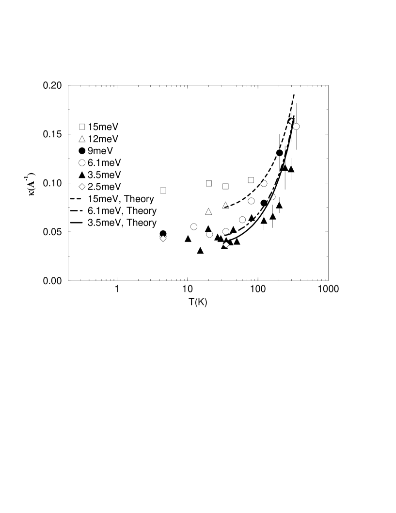
FIG. 5.: A comparison of the NMR-deduced values of the frequency dependence inverse correlations length, $\kappa$, at $\omega$=3.5, 6.1, and 15meV (lines), with the experimental results of Aeppli $et~{}al$[1] (symbols). It is seen that the consistency is quite good at low frequencies, while at high frequencies, the NMR-deduced ${\bf q}$-width is smaller than those seen in neutron scattering experiments.

FIG. 6.: Our calculated spin-lattice relaxation rates $(^{17}T_{1c}T)^{-1}$ for $\rm{}^{17}O$ (solid line) compared to the experimental data of Walstedt $et~{}al$[18] (circles) for $\rm La_{1.85}Sr_{0.15}CuO_{4}$; we use r=0.25 for the calculation. The inset shows the contribution of the AF spin fluctuations (first term only in Eq.(16)) to $(^{17}T_{1c}T)^{-1}$, calculated with the present form factor (r=0.25) and with the standard Shastry-Mila-Rice form factor (r=0).

FIG. 7.: The $\rm{}^{17}O$ spin-lattice relaxation rate ${}^{17}W_{1c}/T$ calculated by assuming r=0.25 (solid line), plotted against the experimental data of Martindale $et~{}al$[3] (circles) for $\rm YBa_{2}Cu_{3}O_{6.96}$. Also shown is the contribution from AF leakage to the relaxation rates ${}^{17}W_{1c}/T$ calculated using our oxygen form factor with r=0.25 and the standard Shastry-Mila-Rice form factor (r=0).

FIG. 8.: The temperature dependence of the oxygen relaxation rate ratios in $\rm YBa_{2}Cu_{3}O_{6.96}$ measured by Martindale $et~{}al$[3], and fits using our theoretical expression Eq(56).

FIG. 9.: The calculated spin-lattice relaxation rates $(^{17}T_{1c}T)^{-1}$ for $\rm YBa_{2}Cu_{3}O_{6.63}$, compared with the data of Takigawa $et~{}al$.[5] The inset shows the predicted anisotropy ratio as described in the text. The predicted anisotropy lies slightly above the calculated curve for $\rm YBa_{2}Cu_{3}O_{6.96}$ in Fig.8, yet both are within the experimental error bars of the $\rm YBa_{2}Cu_{3}O_{6.96}$ data of Martindale $et~{}al$.[3]