Interactions between Membrane Inclusions on Fluctuating Membranes

Abstract

We model membrane proteins as anisotropic objects characterized by symmetric-traceless tensors and determine the coupling between these order-parameters and membrane curvature. We consider the interactions 1) between transmembrane proteins that respect up-down (reflection) symmetry of bilayer membranes and that have circular or non-circular cross-sectional areas in the tangent-plane of membranes, 2) between transmembrane proteins that break reflection symmetry and have circular or non-circular cross-sectional areas, and 3) between non-transmembrane proteins. Using a field theoretic approach, we find non-entropic $1/R^{4}$ interactions between reflection-symmetry-breaking transmembrane proteins with circular cross-sectional area and entropic $1/R^{4}$ interactions between transmembrane proteins with circular cross-section that do not break up-down symmetry in agreement with previous calculations. We also find anisotropic $1/R^{4}$ interactions between reflection-symmetry-conserving transmembrane proteins with non-circular cross-section, anisotropic $1/R^{2}$ interactions between reflection-symmetry-breaking transmembrane proteins with non-circular cross-section, and non-entropic $1/R^{4}$ many-particle interactions among non-transmembrane proteins. For large $R$, these interactions are considerably larger than Van der Waals interactions or screened electrostatic interactions and might provide the dominant force inducing aggregation of the membrane proteins.

I Introduction

Recently, the structure and properties of model and biological membranes have been studied extensively. Biological membranes play a central role in both the structure and function of cells. Biomembranes divide living tissue into different compartments or cells and act as cell boundaries. They determine the nature of all communication between the inside and the outside of cells. This communication can take place via the actual passage of ions or molecules between two compartments or via conformational changes induced in membrane components. Model bilayer lipid membranes in aqueous environments exhibit many of the attributes of the biological membranes. For example, these membranes can form vesicles or more complex structures that divide space into separate compartments, which like cells can fuse or divide. However, there are many properties of biomembranes that cannot be mimicked by lipid bilayers. Energy-driven transport of ions across membranes and receptor-mediated events are only a few of the myriad of membrane-associated functions that lipid bilayers are incapable of performing on their own. Such processes are mediated by proteins that are attached to or dissolved in biological membranes [1, 2, 3, 4, 5]. Thus in order to make lipid bilayers more realistic models of biomembranes, it is necessary to introduce into them membrane inclusions such as proteins.

Membrane proteins are classified as integral proteins or peripheral proteins according to how tightly they are associated with membranes. Integral proteins are so tightly bound to membrane lipids by hydrophobic forces that they can be freed only under denaturing conditions. Peripheral proteins associate with a membrane by binding at the membrane surface; they can be non-destructively dissociated from the membrane by relatively mild procedures. Some integral proteins, known as transmembrane proteins, span the membrane, whereas others are attached to a specific surface of a membrane. For brevity, we refer the latter proteins as non-transmembrane proteins to distinguish these from transmembrane proteins. However, no proteins are known to be completely buried in a membrane [2].

Interactions between membrane proteins is expected to be controlled by lipid affinity, direct interactions such as electrostatic and Van der Waals interactions, and indirect interactions mediated by the membrane [6]. The latter interaction arises from thermally-driven undulations of the membrane and is analogous to the Casimir force between conducting plates. Since the degree to which fluctuations of a membrane are restricted depends on distance between membrane proteins, its free energy also depends on this distance, decreasing with decreasing separation. This implies an attractive force, which leads to a tendency for membrane proteins to aggregate. This indirect interaction between membrane inclusions was first calculated by Goulian, Bruinsma, and Pincus [7]. Before presenting the interaction models introduced in this paper in detail, in Sec.II we will review its results, indicating where they differ from and extend those of Goulian et al. In Sec.III, we introduce a phenomenological model (Model I) for protein interactions. In this model, proteins are characterized by symmetric-traceless tensors depending on the cross-section shapes of proteins on the membrane, and interactions are described by symmetry-allowed couplings between these tensor order-parameters and the curvature tensor of the fluctuating membrane. In Sec.IV, we introduce another phenomenological model (Model II), in which there is an interaction between a membrane protein and membrane lipids at its perimeter. At the perimeter, lipids tend to align with the direction of the protein at a certain angle depending on whether or not proteins break the up-down symmetry of the bilayer membrane. The interaction is described by the fluctuation of the normal vector of the membrane around this preferred direction. The interaction between non-transmembrane proteins is described in Sec.V. Non-transmembrane proteins are proteins with preferred center-of-mass positions not at the center of the bilayer membrane. We expand the potential energy in terms of the deviation from this preferred position and include other couplings considering the symmetry to calculate the interaction between non-transmembrane proteins. Finally, a discussion is given in Sec.VI.

II Review and Summary

A Review of the previous work

The interaction between membrane inclusions with circular cross-section on the membrane has been calculated by Goulian et al. [7]. They use the Helfrich-Canham Hamiltonian [8, 9],

$${\cal H}_{0}=\frac{1}{2}\int d^{2}u\sqrt{g}(\kappa H^{2}+\bar{\kappa}K),$$ (2.1)

to describe fluctuations of the membrane, where $\kappa$ and $\bar{\kappa}$ are the bending and the Gaussian rigidities and $H$ and $K$ are the mean and the Gaussian curvatures, respectively. The surface tension is not taken into account since it effectively vanishes [10, 11]. Within inclusions with circular cross-section, the constants $\kappa$ and $\bar{\kappa}$ are assumed to differ from those of the surrounding membranes. For some inclusions, such as proteins, the circular regions are assumed to be rigid with $\kappa=-\bar{\kappa}=\infty$. This case is the strong-coupling regime. On the other hand, for regions with excess concentrations of lipids, $\kappa$ and $\bar{\kappa}$ within circular regions are assumed to have values close to those of the surrounding membrane. This case is the perturbative regime. In both the strong-coupling and perturbative regimes, Ref. [7] finds that there is an entropic $1/R^{4}$ interaction, which is proportional to the temperature and to the square of the area of the circular region. Also, at low temperatures, there is a non-entropic $1/R^{4}$ interaction between proteins which varies with the square of angle of contact between membrane and proteins. Recently, Golestanian, Goulian, and Kardar [12] extended the calculation in Ref. [7] to the interaction between two rods embedded in a fluctuating membrane. They find an anisotropic $1/R^{4}$ interaction between two rods.

B Summary of the present work

In this paper, we introduce three models for the interaction between membrane inclusions such as transmembrane proteins and non-transmembrane proteins. First, we present Model I. Here, proteins are characterized by symmetric-traceless tensor order-parameters, and the coupling between these order-parameters and membrane curvature is determined by symmetry and power counting. If proteins don’t respect up-down symmetry, we allow for couplings that break up-down symmetry. Otherwise, we require up-down symmetry. For proteins with circular cross-sectional area on the membrane and preserving up-down symmetry, we find the leading distance-dependent free energy,

$${\cal F}=\frac{k_{B}T}{4\pi^{2}\kappa^{2}R^{4}}\int_{D_{1}}d^{2}x\int_{D_{2}}d^{2}y\left[\delta\kappa(x)\delta\bar{\kappa}(y)+\delta\kappa(y)\delta\bar{\kappa}(x)\right],$$ (2.2)

where the coupling constants are denoted in terms of the bending and the Gaussian rigidity differences, $\delta\kappa(x)$ and $\delta\bar{\kappa}(x)$, between proteins and surrounding membrane. This corresponds to the perturbative regime of Ref. [7], whose results we reproduce. For proteins with circular cross-sectional area, up-down-symmetry-breaking couplings do not affect the leading contribution to the free energy, and the leading distance-dependent free energy remains identical to Eq. (2.2). We also calculate interactions between proteins with non-circular cross-sectional area. When up-down symmetry is conserved, we find an interaction energy

$${\cal F} = -k_{B}T\frac{{\cal A}^{2}}{64\pi^{2}\kappa^{2}R^{4}}\left((q_{4}Q_{4}+q_{2}Q_{2}^{2})(q_{4}Q_{4}+q_{2}Q_{2}^{2}+d_{2}Q_{2}^{2})\cos 4(\theta_{1}+\theta_{2})\right.$$ (2.4)

$$\left.+2(q_{4}Q_{4}+q_{2}Q_{2}^{2}+d_{2}Q_{2}^{2})d_{2}Q_{2}^{2}\cos^{2}2\theta_{1}\cos^{2}2\theta_{2}+(q_{2}Q_{2}^{2}+d_{2}Q_{2}^{2})q_{2}Q_{2}^{2}\right),$$

where ${\cal A}$ is the cross-sectional area of proteins, $Q_{2}$ and $Q_{4}$ are magnitudes of 2nd-rank and 4th-rank tensor order parameters measuring orientational anisotropy, respectively, and $\theta_{i}$ are the angles of the directions of proteins measured with respect to the separation vector between proteins (See fig. 1). This anisotropic $1/R^{4}$ interaction contains anisotropic $\cos^{2}2\theta_{1}\cos^{2}2\theta_{2}$ interaction in addition to anisotropic $\cos 4(\theta_{1}+\theta_{2})$ interaction also found in the recent independent work by Golestanian et al. [12]. However, when up-down symmetry is broken, there is an anisotropic $1/R^{2}$ interaction:

$${\cal F}=-\frac{{\cal A}^{2}d_{1}^{2}Q_{2}^{2}}{16\pi\kappa R^{2}}\cos 2(\theta_{1}+\theta_{2}).$$ (2.5)

Thus the leading term in the free energy falls off with separation as $1/R^{2}$ rather than $1/R^{4}$.

Next, we introduce Model II in which we impose a certain boundary condition at the perimeter of proteins with the circular cross-sectional area. For proteins with up-down symmetry, we find

$${\cal F}=-k_{B}T\frac{6{\cal A}^{2}}{\pi^{2}R^{4}}.$$ (2.6)

This free energy looks similar to that of Ref. [7] in the strong-coupling regime. When proteins break up-down symmetry, we find

$${\cal F}=-k_{B}T\frac{6{\cal A}^{2}}{\pi^{2}R^{4}}+\frac{4\kappa{\cal A}^{2}}{\pi}\frac{\alpha_{1}^{2}+\alpha_{2}^{2}}{R^{4}},$$ (2.7)

where $\alpha_{i}$ is the contact angle between the direction of $i$-th protein and the unit normal of the membrane (See fig. 2). In the limit $T\rightarrow 0$, this free energy becomes the result in Ref. [7] for the low-temperature regime.

Finally, we introduce a height-displacement model in which protein positions normal to the membrane can vary. In this model, we find three- and four-body interactions in addition to a two-body interaction. These three- and four-body interactions also fall off as $1/R^{4}$ and are the same order of magnitude as two-body interaction.

Consequently, by introducing three models to describe the interaction between membrane inclusions such as proteins, we recover all the results in Ref. [7]. Furthermore, we obtain anisotropic interactions between proteins with non-circular cross-sectional area. Also, we extend the calculation to the up-down symmetry breaking proteins with non-circular cross-section and find anisotropic $1/R^{2}$ interaction between them. Moreover, using a height-displacement model, we find three- and four-body $1/R^{4}$ interaction in addition to two-body $1/R^{4}$ interaction.

III Model I

For a fluid membrane free of membrane proteins, the energy of membrane conformations can be described by the Helfrich-Canham Hamiltonian [8, 9],

$${\cal H}_{0}=\frac{1}{2}\int d^{2}u\sqrt{g}(\kappa H^{2}+\bar{\kappa}K),$$ (3.1)

expressed in terms of the local mean and Gaussian curvatures. We will work at length scales large compared with the membrane thickness but small compared with the membrane’s persistence length. Thus, we can parameterize the membrane in the Monge gauge ${\bf R}=({\bf x},h({\bf x}))$ where ${\bf x}=(u_{1},u_{2})$. In terms of ${\bf R}$ and the unit normal vector of the membrane ${\bf N}$, the metric tensor $g_{\alpha\beta}$ is given by $\partial_{\alpha}{\bf R}\cdot\partial_{\beta}{\bf R}$ and the curvature tensor $K_{\alpha\beta}$ is given by ${\bf N}\cdot D_{\alpha}D_{\beta}{\bf R}$, where $D_{\alpha}$ is the covariant derivative along $u_{\alpha}$ direction on the membrane. In the Monge gauge,

$$H=\frac{1}{2}g^{\alpha\beta}K_{\alpha\beta}=\nabla^{2}h+O(h^{2}),$$ (3.2)

$$K=\det g^{\alpha\beta}K_{\beta\gamma}=\nabla^{2}h\nabla^{2}h-\partial_{\alpha}\partial_{\beta}h\partial_{\alpha}\partial_{\beta}h+O(h^{4}).$$ (3.3)

When the topology of the membrane is fixed, the Gaussian curvature term can be dropped, and the leading term in ${\cal H}_{0}$ in an expansion in derivatives of $h$ is

$${\cal H}_{0}=\frac{1}{2}\kappa\int d^{2}x\nabla^{2}h\nabla^{2}h.$$ (3.4)

Now let us consider the coupling between membrane proteins and membranes.

A Proteins with circular cross-section

Membrane proteins can have arbitrary shapes; as a result their tangent-plane cross-sections can be any shape. Now we will compute the undulation mediated force between proteins separated by a distance larger than the size of proteins. For simplicity, let us first consider membrane proteins that have a circular cross-sectional area on the membrane. These proteins may be described by a scalar density, $\rho$, which may be interpreted as the distribution function of proteins describing the positions of proteins and the configurations of protein’s amino acid sequence

$$\rho({\bf x})=\sum_{i}\frac{1}{\sqrt{g}}f_{i}({\bf x}-{\bf x}_{i}),$$ (3.5)

where ${\bf x}=(u^{1},u^{2})$ is a point on the membrane and the sum is over all proteins. The specific form of $f_{i}({\bf x}-{\bf x}_{i})$ depends on the specific conformation of $i$-th protein at the position ${\bf x}_{i}$. It vanishes outside the protein cross section:

$$f_{i}({\bf x})=\left\{\begin{array}[]{ll}f(x),&|{\bf x}|<a_{p},\\ 0,&|{\bf x}|>a_{p}.\end{array}\right.$$ (3.6)

where $a_{p}=\sqrt{{\cal A}/\pi}$ is the radius of the protein where ${\cal A}$ is its cross-sectional area. We assume all proteins are identical so that they are all described by the the same function $f(|{\bf x}-{\bf x}_{i}|)$. For membrane proteins, $a_{p}$ is of order $10^{2}\AA$. If we model the protein as a uniform cylinder, the distribution function of protein will be $f(x)=1$ inside the projected area and $f(x)=0$ outside. In general, proteins have non-uniform folding of the amino acid chain, and $f(x)$ will have small deviations from unity inside the circular cross-sectional region $D$. In this case, we use

$$\int_{D}d^{2}xf(x)={\cal A}$$ (3.7)

as the definition of ${\cal A}$.

When proteins do not break up-down symmetry, the relevant coupling between $\rho$ and the height fluctuation field of the membrane is

$${\cal H}_{\rm int} = \frac{1}{2}\int d^{2}x[\alpha\rho({\bf x})K_{a}^{a}K_{b}^{b}+\gamma\rho({\bf x})K_{b}^{a}K_{a}^{b}]$$ (3.8)

$$= \frac{1}{2}\sum_{i}\int_{D_{i}}d^{2}x[\alpha f(|{\bf x}-{\bf x}_{i}|)K^{a}_{a}K^{b}_{b}+\gamma f(|{\bf x}-{\bf x}_{i}|)K^{a}_{b}K^{b}_{a}],$$ (3.9)

where $D_{i},i=1,2,\cdots$ denote circular regions occupied by membrane proteins. The coupling constants $\alpha$ and $\gamma$ describe couplings between the density inside protein’s cross section and the curvature of a membrane. Thus these can be related to the bending and Gaussian rigidities:

$$\alpha f(x)=\delta\kappa(x)+\delta\bar{\kappa}(x)\;\;,\;\;\;\gamma f(x)=-\delta\bar{\kappa}(x)\;,$$ (3.10)

where $\delta\kappa$ and $\delta\bar{\kappa}$ can be interpreted as the changes in the bending and the Gaussian rigidities due to the existence of proteins on the membrane. In the Monge gauge, to lowest order in $h$

$$K^{a}_{a}=-\nabla^{2}h\;\;,\;\;\;K^{a}_{b}K^{b}_{a}=\partial_{a}\partial_{b}h\partial_{a}\partial_{b}h,$$ (3.11)

and the relevant coupling becomes

$${\cal H}_{\rm int}=\frac{1}{2}\int d^{2}x[\alpha\rho({\bf x})(\nabla^{2}h)^{2}+\gamma\rho({\bf x})\partial_{a}\partial_{b}h\partial_{a}\partial_{b}h].$$ (3.12)

The free energy is given by

$$\exp[-\beta{\cal F}] = \int[{\cal D}h]\exp[-\frac{1}{2}\beta\kappa\int d^{2}x(\nabla^{2}h)^{2}$$ (3.14)

$$-\frac{1}{2}\beta\int d^{2}x[\alpha\rho({\bf x})(\nabla^{2}h)^{2}+\gamma\rho({\bf x})\partial_{a}\partial_{b}h\partial_{a}\partial_{b}h].$$

We can use the cumulant expansion to calculate this form of the free energy. We write

$$e^{-\beta({\cal F}-{\cal F}_{0})}=\left\langle\exp[-\frac{1}{2}\beta\int d^{2}x[\alpha\rho({\bf x})(\nabla^{2}h)^{2}+\gamma\rho({\bf x})\partial_{a}\partial_{b}h\partial_{a}\partial_{b}h]]\right\rangle_{0}$$ (3.15)

where $\langle\rangle_{0}$ denotes the ensemble average over the fluid membrane Hamiltonian only and

$$e^{-\beta{\cal F}_{0}}=\int[{\cal D}h]\exp[-\frac{1}{2}\beta\kappa\int d^{2}x(\nabla^{2}h)^{2}].$$ (3.16)

The cumulant expansion gives

$$\langle e^{V}\rangle_{0} = \langle 1+V+\frac{1}{2}V^{2}+\cdots\rangle_{0}$$ (3.17)

$$= \exp\left[\langle V\rangle_{0}+\frac{1}{2}[\langle V^{2}\rangle_{0}-\langle V\rangle_{0}^{2}]+{\cal O}(V^{3})\right].$$ (3.18)

Plugging Eq. (3.15) into the cumulant expansion Eq. (3.18) and keeping terms up to order $h^{4}$, we find the free energy

$$-\beta({\cal F}-{\cal F}_{0}) = \left\langle-\frac{1}{2}\beta\int d^{2}x[\alpha\rho({\bf x})(\nabla^{2}h)^{2}+\gamma\rho({\bf x})\partial_{a}\partial_{b}h\partial_{a}\partial_{b}h]\right\rangle_{0}$$ (3.21)

$$+\frac{1}{2}\left\langle(-\frac{1}{2}\beta\int d^{2}x[\alpha\rho({\bf x})(\nabla^{2}h)^{2}+\gamma\rho({\bf x})\partial_{a}\partial_{b}h\partial_{a}\partial_{b}h])^{2}\right\rangle_{0}$$

$$-\frac{1}{2}\left\langle-\frac{1}{2}\beta\int d^{2}x[\alpha\rho({\bf x})(\nabla^{2}h)^{2}+\gamma\rho({\bf x})\partial_{a}\partial_{b}h\partial_{a}\partial_{b}h]\right\rangle_{0}^{2}.$$

This can be expanded in terms of the height correlation function $G_{hh}({\bf x}-{\bf y})$ and its derivatives. The height correlation function in the real space is

$$G_{hh}({\bf x}-{\bf y}) = \langle h({\bf x})h({\bf y})\rangle_{0}$$ (3.22)

$$= \int\frac{d^{2}p}{(2\pi)^{2}}\frac{d^{2}q}{(2\pi)^{2}}e^{i{\bf p}\cdot{\bf x}+i{\bf q}\cdot{\bf y}}\langle h({\bf p})h({\bf q})\rangle_{0}$$ (3.23)

$$= \int\frac{d^{2}p}{(2\pi)^{2}}\frac{e^{i{\bf p}\cdot({\bf x}-{\bf y})}}{\beta\kappa p^{4}}=\frac{1}{16\pi\beta\kappa}R^{2}\ln R^{2},$$ (3.24)

where we used $\langle h({\bf p})h({\bf q})\rangle_{0}=(2\pi)^{2}\delta({\bf p}+{\bf q})/\beta\kappa p^{4}$ in momentum space and ${\bf x}-{\bf y}={\bf R}$. Then, taking derivatives we find

$$\langle\partial_{a}\partial_{b}h({\bf x})\partial_{i}\partial_{j}h({\bf y})\rangle_{0} = \partial_{a}\partial_{b}\partial_{i}\partial_{j}G_{hh}({\bf x}-{\bf y})$$ (3.25)

$$= \frac{1}{4\pi\beta\kappa R^{2}}\left[(\delta_{ab}\delta_{ij}+\delta_{ai}\delta_{bj}+\delta_{aj}\delta_{bi})\right.$$ (3.28)

$$-2(\hat{R}_{a}\hat{R}_{b}\delta_{ij}+\hat{R}_{a}\hat{R}_{i}\delta_{bj}+\hat{R}_{a}\hat{R}_{j}\delta_{bi}+\hat{R}_{b}\hat{R}_{i}\delta_{aj}+\hat{R}_{b}\hat{R}_{j}\delta_{ai}+\hat{R}_{i}\hat{R}_{j}\delta_{ab})$$

$$\left.+8\hat{R}_{a}\hat{R}_{b}\hat{R}_{i}\hat{R}_{j}\right]$$

$$\equiv \frac{1}{4\pi\beta\kappa R^{2}}T_{abij}(\hat{{\bf R}}),$$ (3.29)

where $\hat{{\bf R}}={\bf R}/R$, $R=|{\bf R}|$. We proceed to calculate the terms in Eq. (3.21). We are only interested in terms that depend on the distance between membrane proteins. We can, therefore, drop the first and the last terms in the RHS of Eq. (3.21) since they do not depend on distance:

$$\left\langle\int d^{2}x\rho({\bf x})\partial_{a}\partial_{b}h\partial_{a}\partial_{b}h\right\rangle_{0} = \int d^{2}x\rho({\bf x})\nabla^{4}G_{hh}({\bf x}-{\bf y})|_{{\bf y}={\bf x}}$$ (3.30)

$$= \int d^{2}x\rho(x)\int\frac{d^{2}p}{(2\pi)^{2}}\frac{1}{\beta\kappa}=\sum_{i}\int_{D_{i}}d^{2}xf(x)\int\frac{d^{2}p}{(2\pi)^{2}}\frac{1}{\beta\kappa}$$ (3.31)

$$= \frac{N}{(2\pi)^{2}\beta\kappa}\pi a_{p}^{2}\pi\Lambda^{2}=\frac{N}{4\beta\kappa}(a_{p}\Lambda)^{2},$$ (3.32)

and similarly

$$\left\langle\int d^{2}x\rho({\bf x})(\nabla^{2}h)^{2}\right\rangle_{0}=\frac{N}{4\beta\kappa}(a_{p}\Lambda)^{2},$$ (3.33)

where $N$ is the number of proteins. In Eq. (3.32) we introduced the cut-off for the height fluctuation field $\Lambda\sim 1/a_{p}$ where $a_{p}$ is the radius of the protein. The second term gives contribution to the distance-dependent free energy:

$$\frac{\beta^{2}}{8}\int d^{2}xd^{2}y\rho({\bf x})\rho({\bf y})\left[4\alpha\gamma\partial_{a}\partial_{b}\nabla^{2}G_{hh}({\bf x}-{\bf y})\partial_{a}\partial_{b}\nabla^{2}G_{hh}({\bf x}-{\bf y})\right.$$ (3.35)

$$\left.+2\gamma^{2}\partial_{a}\partial_{b}\partial_{i}\partial_{j}G_{hh}({\bf x}-{\bf y})\partial_{a}\partial_{b}\partial_{i}\partial_{j}G_{hh}({\bf x}-{\bf y})\right]$$

$$= \frac{\beta^{2}}{8}\int d^{2}xd^{2}y\rho({\bf x})\rho({\bf y})\frac{1}{(4\pi\beta\kappa R^{2})^{2}}\left[4\alpha\gamma T_{abii}(\hat{\bf R})T_{abjj}(\hat{\bf R})+2\gamma^{2}T_{abij}(\hat{\bf R})T_{abij}(\hat{\bf R})\right],$$ (3.36)

where we kept only the leading distance-dependent terms and ${\bf R}={\bf x}-{\bf y}$. Thus, the leading distance-dependent free energy is given by

$$-\beta{\cal F}=\frac{1}{4}\int d^{2}x\int d^{2}y\rho({\bf x})U(|{\bf x}-{\bf y}|)\rho({\bf y}),$$ (3.37)

where

$$U(|{\bf x}-{\bf y}|)=\frac{(\alpha\gamma+\gamma^{2})}{(\pi\kappa)^{2}|{\bf x}-{\bf y}|^{4}}.$$ (3.38)

For two proteins separated by a distance $R$, the leading $R$ dependence is

$$-\beta{\cal F}=\frac{1}{2\pi^{2}\kappa^{2}R^{4}}\int_{D_{1}}d^{2}x\int_{D_{2}}d^{2}y\left[\alpha\gamma+\gamma^{2}\right]f(x)f(y).$$ (3.39)

Relating the couplings $\alpha$ and $\gamma$ with the variations of the bending rigidity and the Gaussian rigidity as in Eq. (3.10), we recover the result of Goulian et al. [7]

$${\cal F}=\frac{k_{B}T}{4\pi^{2}\kappa^{2}R^{4}}\int_{D_{1}}d^{2}x\int_{D_{2}}d^{2}y\left[\delta\kappa(x)\delta\bar{\kappa}(y)+\delta\kappa(y)\delta\bar{\kappa}(x)\right].$$ (3.40)

If membrane proteins break up-down bilayer symmetry, there is another possible relevant coupling,

$${\cal H}_{\rm int}=\frac{1}{2}\lambda\int d^{2}x\rho({\bf x})K^{a}_{a}=\frac{1}{2}\lambda\sum_{i}\int_{D_{i}}d^{2}xf(|{\bf x}-{\bf x}_{i}|)K^{a}_{a}.$$ (3.41)

However, this term does not contribute to protein-protein interactions since the distance-dependent contribution vanishes as follows,

$$\int d^{2}xd^{2}y\rho({\bf x})\rho({\bf y})\langle\nabla^{2}h({\bf x})\nabla^{2}h({\bf y})\rangle_{0} = \int d^{2}xd^{2}y\rho({\bf x})\rho({\bf y})\nabla^{4}G_{hh}({\bf x}-{\bf y})$$ (3.42)

$$= \frac{2}{\beta\kappa}\int_{D_{1}}d^{2}x\int_{D_{2}}d^{2}yf(x)f(y)\delta(x-y)=0.$$ (3.43)

B Proteins with non-circular cross-sections

So far we have, for simplicity, considered protein-protein interactions when proteins have circular cross section. However, in general proteins have asymmetric conformations giving rise to non-circular foot prints on the membrane surface. They can then be characterized by symmetric-traceless tensor order-parameters such as $\tilde{Q}^{ab},\tilde{Q}^{abcd}$, and so on:

$$\tilde{Q}^{ab}({\bf x})=\sum_{\mu}\frac{1}{\sqrt{g}}Q^{ab}_{\mu}f({\bf x}-{\bf x}_{\mu}),\;\;\;\tilde{Q}^{abcd}({\bf x})=\sum_{\mu}\frac{1}{\sqrt{g}}Q^{abcd}_{\mu}f({\bf x}-{\bf x}_{\mu}),$$ (3.44)

where ${\bf x}_{\mu}$ denotes the position of $\mu$-th protein and $Q^{ab}_{\mu}$ and $Q^{abcd}_{\mu}$ are the symmetric-traceless tensors constructed from the characteristic direction vector of $\mu$-th protein on the membrane.

When up-down symmetry is not broken, the relevent coupling between inclusions and curvature is

$${\cal H}_{\rm int}=\frac{1}{2}\int d^{2}x\tilde{S}^{abcd}({\bf x})K_{ab}K_{cd},$$ (3.45)

where

$$\tilde{S}^{abcd}({\bf x})=q_{4}\tilde{Q}^{abcd}({\bf x})+q_{2}\tilde{Q}^{ab}({\bf x})\tilde{Q}^{cd}({\bf x})+d_{2}\tilde{Q}^{ac}({\bf x})\tilde{Q}^{bd}({\bf x}).$$ (3.46)

The coupling constants $q_{4}$, $q_{2}$ and $d_{2}$ describe couplings between the protein tensor order parameters and the curvature of a membrane. Results for membranes with circular cross-sections can be obtained by choosing

$$S^{abcd}_{\mu}=\alpha\delta^{ab}\delta^{cd}+\gamma\delta^{ac}\delta^{bd},$$ (3.47)

rather than insisting the order parameters be symmetric and traceless. With this coupling, we proceed as before using the cumulant expansion. For two proteins separated by a distance vector ${\bf R}$ from one to the other, the free energy becomes

$$-\beta{\cal F} = \frac{\beta^{2}}{8}\int d^{2}x\int d^{2}y\tilde{S}^{abcd}({\bf x})\tilde{S}^{ijkl}({\bf y})\langle\partial_{a}\partial_{b}h({\bf x})\partial_{c}\partial_{d}h({\bf x})\partial_{i}\partial_{j}h({\bf y})\partial_{k}\partial_{l}h({\bf y})\rangle_{0}$$ (3.48)

$$= \frac{\beta^{2}}{8}\int d^{2}x\int d^{2}y\tilde{S}^{abcd}({\bf x})\tilde{S}^{ijkl}({\bf y})\partial_{a}\partial_{b}\partial_{i}\partial_{j}G_{hh}({\bf x}-{\bf y})\partial_{a}\partial_{b}\partial_{i}\partial_{j}G_{hh}({\bf x}-{\bf y}).$$ (3.49)

In terms of the tensor $T_{abij}$ introduced before, the final form for the free energy writes as

$$-\beta{\cal F}=\frac{1}{4}\int d^{2}x\int d^{2}y\tilde{S}^{abcd}({\bf x})U_{abcd,ijkl}(|{\bf x}-{\bf y}|)\tilde{S}^{ijkl}({\bf y}),$$ (3.50)

where

$$U_{abcd,ijkl}(|{\bf x}-{\bf y}|)=\frac{(T_{abij}(\hat{\bf R})T_{cdkl}(\hat{\bf R})+T_{abkl}(\hat{\bf R})T_{cdij}(\hat{\bf R}))}{8\pi^{2}\kappa^{2}|{\bf x}-{\bf y}|^{4}}.$$ (3.51)

For two identical proteins separated by ${\bf R}={\bf x}_{1}-{\bf x}_{2}$, the leading distance-dependent free energy is found to be

$${\cal F}=-k_{B}T\frac{{\cal A}^{2}S^{abcd}({\bf x}_{1})S^{ijkl}({\bf x}_{2})}{64\pi^{2}\kappa^{2}R^{4}}[T_{abij}(\hat{\bf R})T_{cdkl}(\hat{\bf R})+T_{abkl}(\hat{\bf R})T_{cdij}(\hat{\bf R})].$$ (3.52)

Now the free energy is anisotropic, depending on the direction of the separation vector ${\bf R}$ and the orientation of proteins described by $S^{abcd}({\bf x}_{i})$. $Q^{abcd}$ is a 4th-rank symmetric-traceless tensor, which can be expressed as

$$Q^{abcd} = Q_{4}\left(e^{a}e^{b}e^{c}e^{d}\right.$$ (3.55)

$$-\frac{1}{6}(e^{a}e^{b}\delta^{cd}+e^{a}e^{c}\delta^{bd}+e^{a}e^{d}\delta^{bc}+e^{b}e^{c}\delta^{ad}+e^{b}e^{d}\delta^{ac}+e^{c}e^{d}\delta^{ab})$$

$$\left.+\frac{1}{24}(\delta^{ab}\delta^{cd}+\delta^{ac}\delta^{bd}+\delta^{ad}\delta^{bc})\right),$$

and $Q^{ab}$ is a 2nd-rank symmetric-traceless tensor;

$$Q^{ab}=Q_{2}\left(e^{a}e^{b}-\frac{1}{2}\delta^{ab}\right),$$ (3.56)

where $e^{1}=\cos\theta$ and $e^{2}=\sin\theta$ characterize the direction of protein with $\theta$ measured with respect to the separation vector ${\bf R}$ and $Q_{2}$ and $Q_{4}$ are magnitudes of 2-fold and 4-fold anisotropy, respectively. Then, the free energy becomes

$${\cal F} = -k_{B}T\frac{{\cal A}^{2}}{64\pi^{2}\kappa^{2}R^{4}}\left((q_{4}Q_{4}+q_{2}Q_{2}^{2})(q_{4}Q_{4}+q_{2}Q_{2}^{2}+d_{2}Q_{2}^{2})\cos 4(\theta_{1}+\theta_{2})\right.$$ (3.58)

$$\left.+2(q_{4}Q_{4}+q_{2}Q_{2}^{2}+d_{2}Q_{2}^{2})d_{2}Q_{2}^{2}\cos^{2}2\theta_{1}\cos^{2}2\theta_{2}+(q_{2}Q_{2}^{2}+d_{2}Q_{2}^{2})q_{2}Q_{2}^{2}\right),$$

Again, for proteins breaking up-down symmetry, we have the additional relevant coupling

$${\cal H}_{\rm int}=\frac{1}{2}\int d^{2}x\tilde{S}^{ab}({\bf x})K_{ab}.$$ (3.59)

In contrast to the case of circular cross section, this coupling leads to a qualitative change in the protein-protein interaction. Proceeding as above, we find the leading distance dependence of protein inteaction is $1/R^{2}$:

$$-\beta{\cal F} = \frac{\beta^{2}}{4}\int d^{2}x\int d^{2}y\tilde{S}^{ab}({\bf x})\tilde{S}^{ij}({\bf y})\langle\partial_{a}\partial_{b}h({\bf x})\partial_{i}\partial_{j}h({\bf y})\rangle_{0}$$ (3.60)

$$= \frac{\beta^{2}}{4}\int d^{2}x\int d^{2}y\tilde{S}^{ab}({\bf x})\tilde{S}^{ij}({\bf y})\partial_{a}\partial_{b}\partial_{i}\partial_{j}G_{hh}({\bf x}-{\bf y})$$ (3.61)

$$= \frac{1}{4}\int d^{2}x\int d^{2}y\tilde{S}^{ab}({\bf x})U_{ab,ij}(|{\bf x}-{\bf y}|)\tilde{S}^{ij}({\bf y}),$$ (3.62)

where

$$U_{ab,ij}(|{\bf x}-{\bf y}|)=\frac{\beta T_{abij}(\hat{\bf R})}{2\pi\kappa|{\bf x}-{\bf y}|^{2}}.$$ (3.63)

This interaction is also anisotropic, depending on ${\bf R}$ and $S^{ab}({\bf x}_{i})$. For spherical cross section, since $S^{ab}\sim\delta_{ab}$ and $\delta^{ab}\delta^{ij}T_{abij}=0$, the contribution to the interaction vanishes as before. For ellipsoidal cross section, $S^{ab}=d_{1}Q^{ab}$ where $d_{1}$ is the coupling constant and the free energy becomes

$${\cal F}=-\frac{{\cal A}^{2}d_{1}^{2}Q_{2}^{2}}{16\pi\kappa R^{2}}\cos 2(\theta_{1}+\theta_{2}).$$ (3.64)

The minimum energy configurations are at $\theta_{1}+\theta_{2}=0,\pi$.

Consequently, by introducing symmetric-traceless tensors as the order-parameters for anisotropic proteins and by determining the relevant couplings by symmetry, we were able to rederive the results for the circular cross section by Goulian et al. [7]. Furthermore, we obtained anisotropic interactions between proteins which have the non-circular cross section. This anisotropic interaction has the leading distance dependence $1/R^{4}$ and $1/R^{2}$ depending on up-down symmetry breaking.

IV Model II

In the previous section, we introduced a coupling between membrane proteins and the height fluctuation field of the membrane by considering symmetry and power counting. Since the order parameter for proteins in the coupling Eq. (3.9) can be interpreted as the distribution function of proteins, the physical implication of this coupling can be that the bending and Gaussian rigidities inside the protein cross section differ slightly from those of the surrounding membrane. Thus this coupling can be thought of as perturbative. However, if proteins are infinitely rigid with $\kappa=-\bar{\kappa}=\infty$ inside the protein cross section, perturbation theory fails. In this case, we can derive the protein-protein interaction by considering the phenomenological interaction between membrane proteins and membrane lipids at the perimeter of the proteins.

First, let us consider proteins which have circular cross sections and do not break up-down symmetry. These proteins can be modelled as inversion-symmetric three-dimensional ellipsoids of revolution (or cylinder) with a major axis pointing along a unit vector ${\bf m}$ in three-dimensions. Their orientational order can be characterized by the symmetric-traceless tensor $Q_{ij}=(m_{i}m_{j}-\delta_{ij}/3)$. We assume the axis ${\bf m}$ prefers to align along the membrane normal ${\bf N}$. A simple interaction favoring this alignment is

$${\cal H}_{\rm int}=-\frac{1}{2}\alpha\sum_{\mu}\int_{c_{\mu}}\frac{dl}{2\pi a_{p}}Q^{ij}N_{i}N_{j}.$$ (4.1)

In the Monge gauge,

$$Q^{ij}N_{i}N_{j}=({\bf m}\cdot{\bf N})^{2}-\frac{1}{3}=-\delta^{ab}(m_{a}-N_{a})(m_{b}-N_{b})+\mbox{constant},$$ (4.2)

where $a,b$ run over 1,2 only and $N_{a}=-\partial_{a}h$ to lowest order in $h$. Now we can Taylor-expand the unit normal of the membrane at the perimeter from the center of the protein to lowest non-trivial order in $a_{p}$

$$N_{a}({\bf r})|_{c_{\mu}}=N_{a}({\bf R}_{\mu}+a_{p}{\bf b}(1-({\bf b}\cdot{\bf m}_{\perp})^{2})^{1/2})=N_{a}({\bf R}_{\mu})+a_{p}{\bf b}\cdot\nabla N_{a}+\cdots,$$ (4.3)

where ${\bf b}$ is the unit vector from the center of the protein to its perimeter and $N_{a}({\bf R}_{\mu})$ is the average of $N_{a}({\bf r})$ along the perimeter $c_{\mu}$. Dropping the constant term, the coupling becomes

$${\cal H}_{\rm int} = \alpha\sum_{\mu}\int_{c_{\mu}}\frac{dl}{2\pi a_{p}}\left[m_{a}({\bf R}_{\mu})-N_{a}({\bf R}_{\mu})-a_{p}b_{b}\partial_{b}N_{a}\right]^{2}$$ (4.4)

$$= \alpha\sum_{\mu}\left[\tilde{m}_{a}({\bf R}_{\mu})\tilde{m}_{a}({\bf R}_{\mu})+\frac{a_{p}^{2}}{2}\partial_{b}N_{a}\partial_{b}N_{a}\right],$$ (4.5)

where $\tilde{m}_{a}({\bf R}_{\mu})=m_{a}({\bf R}_{\mu})-N_{a}({\bf R}_{\mu})$. The free energy is

$$e^{-\beta{\cal F}} = \int[{\cal D}h][{\cal D}\tilde{m}_{a}({\bf R}_{\mu})]e^{-\beta{\cal H}_{0}-\beta{\cal H}_{\rm int}}$$ (4.6)

$$= ({\rm constant})\int[{\cal D}h]\exp[-\frac{1}{2}\beta\kappa\int d^{2}x(\nabla^{2}h)^{2}-\frac{1}{2\pi}\beta\alpha{\cal A}\sum_{\mu}\partial_{b}N_{a}({\bf R}_{\mu})\partial_{b}N_{a}({\bf R}_{\mu})],$$ (4.7)

where ${\cal H}_{0}=\frac{1}{2}\kappa\int d^{2}x(\nabla^{2}h)^{2}$ and the integration over $\tilde{m}_{a}$ is trivial and gives constant contribution. Since the coupling has a quadratic form, we can evaluate this using the Hubbard-Stratonovich transformation. Although it is nothing more than completing the square, we will find this technique to be very useful. By introducing the auxiliary fields ${\bf W}(\mu)$ and defining ${\bf V}(\mu)$ as

$$V_{1}(\mu)=\partial_{1}N_{1}(\mu)\;\;,\;\;V_{2}(\mu)=\sqrt{2}\partial_{1}N_{2}(\mu)=\sqrt{2}\partial_{2}N_{1}(\mu)\;\;,\;\;V_{3}(\mu)=\partial_{2}N_{2}(\mu)\;\;,$$ (4.8)

we have

$$e^{-\beta{\cal F}} = \int[{\cal D}h][{\cal D}{\bf W}(\mu)]\exp[-\beta{\cal H}_{0}-\frac{1}{2\Gamma}\sum_{\mu}{\bf W}(\mu)\cdot{\bf W}(\mu)+i\sum_{\mu}{\bf W}(\mu)\cdot{\bf V}(\mu)]$$ (4.9)

$$= e^{-\beta{\cal F}_{0}}\int[{\cal D}{\bf W}(\mu)]\exp[-\frac{1}{2\Gamma}\sum_{\mu}{\bf W}(\mu)\cdot{\bf W}(\mu)]\langle\exp[i\sum_{\mu}{\bf W}(\mu)\cdot{\bf V}(\mu)]\rangle_{0},$$ (4.10)

where $\Gamma=\beta\alpha{\cal A}/\pi$. Using the cumulant expansion again, to the lowest order we obtain

$$e^{-\beta({\cal F}-{\cal F}_{0})} = \int[{\cal D}{\bf W}(\mu)]\exp[-\langle\frac{1}{2}\sum_{\mu,\nu}{\bf W}(\mu)\cdot{\bf V}(\mu){\bf W}(\nu)\cdot{\bf V}(\nu)\rangle_{0}]$$ (4.11)

$$= \int[{\cal D}{\bf W}(\mu)]\exp[-\frac{1}{2}\sum_{\mu,\nu}W_{a}(\mu)\langle V_{a}(\mu)V_{b}(\nu)\rangle_{0}W_{b}(\nu)].$$ (4.12)

For two proteins separated by a distance $R$, we find

$$e^{-\beta({\cal F}-{\cal F}_{0})} = \int[{\cal D}{\bf W}(1)][{\cal D}{\bf W}(2)]\exp[-\frac{1}{2}\sum_{\mu,\nu=1}^{2}W_{a}(\mu)\langle V_{a}(\mu)V_{b}(\nu)\rangle_{0}W_{b}(\nu)]$$ (4.13)

$$= \left(\det\langle V_{a}(\mu)V_{b}(\nu)\rangle_{0}\right)^{-1/2}$$ (4.14)

$$= ({\rm constant})\left(1-3(\frac{8}{R^{2}\Lambda^{2}})^{2}\right)^{-1/2},$$ (4.15)

where $\Lambda\sim 1/a_{p}$ is a cut-off for the height fluctuation, and $a_{p}$ is the radius of the protein introduced in Sec. II.A. Thus, the free energy has an $R$-dependence as

$${\cal F}=-k_{B}T\frac{96}{R^{4}\Lambda^{4}}=-k_{B}T\frac{6{\cal A}^{2}}{\pi^{2}R^{4}},$$ (4.16)

in accord with the previous calculation by Goulian et al. [7]. In the above equation, we used a cut-off for the height fluctuation, $\Lambda=2/a_{p}$ [13].

For proteins that break the up-down symmetry, the unit normal of the membrane at the perimeter of the protein is not forced to be parallel to the direction of the protein. Instead, the unit normal is forced to have a fixed angle $\alpha_{\mu}$ with the direction of the $\mu$-th protein. Thus the preferred unit normal at the perimeter is

$${\bf N}_{0}({\bf r})|_{c_{i}}=\frac{{\bf m}+\alpha_{\mu}{\bf b}}{\sqrt{1+\alpha_{\mu}^{2}}}.$$ (4.17)

The coupling between the protein and the membrane at the perimeter of the protein is

$${\cal H}_{\rm int}=\alpha\sum_{\mu}\int_{c_{\mu}}\frac{dl}{2\pi a_{p}}({\bf N}-{\bf N}_{0})^{2}.$$ (4.18)

We Taylor expand to find to lowest order

$${\cal H}_{\rm int} = \alpha\sum_{\mu}\int_{c_{\mu}}\frac{dl}{2\pi a_{p}}[(m_{a}-N_{a})(m_{a}-N_{a})-2\alpha_{\mu}N_{a}b_{a}]$$ (4.19)

$$= \alpha\sum_{\mu}[\tilde{m}_{a}(\mu)\tilde{m}_{a}(\mu)+\frac{1}{2}a_{p}^{2}\partial_{b}N_{a}\partial_{b}N_{a}-a_{p}\alpha_{\mu}\partial_{a}N_{a}].$$ (4.20)

The free energy is now

$$e^{-\beta{\cal F}} = \int[{\cal D}h][{\cal D}\tilde{m}_{a}(\mu)]\exp[-\frac{1}{2}\beta\kappa\int d^{2}x(\nabla^{2}h)^{2}$$ (4.22)

$$-\beta\alpha\sum_{\mu}[\tilde{m}_{a}(\mu)\tilde{m}_{a}(\mu)+\frac{1}{2}a_{p}^{2}\partial_{b}N_{a}\partial_{b}N_{a}-a_{p}\alpha_{\mu}\partial_{a}N_{a}]]$$

$$= \int[{\cal D}h]\exp\left[-\frac{1}{2}\beta\kappa\int d^{2}x(\nabla^{2}h)^{2}-\frac{\beta\alpha{\cal A}}{2\pi}\sum_{\mu}[\partial_{b}N_{a}\partial_{b}N_{a}-\frac{2\alpha_{\mu}}{a_{p}}\partial_{a}N_{a}]\right].$$ (4.23)

Re-defining ${\bf V}(\mu)$ as

$$V_{1}(\mu)=\partial_{1}N_{1}(\mu)-\frac{\alpha_{\mu}}{a_{p}}\;\;,\;\;V_{2}(\mu)=\partial_{1}N_{2}(\mu)=\partial_{2}N_{1}(\mu)\;\;,\;\;V_{3}(\mu)=\partial_{2}N_{2}(\mu)-\frac{\alpha_{\mu}}{a_{p}}\;\;,$$ (4.24)

the free energy becomes

$$e^{-\beta{\cal F}} = \int[{\cal D}h]\exp\left[-\frac{1}{2}\beta\kappa\int d^{2}x(\nabla^{2}h)^{2}-\frac{\beta\alpha{\cal A}}{2\pi}\sum_{\mu}{\bf V}(\mu)\cdot{\bf V}(\mu)\right]$$ (4.25)

$$= \int[{\cal D}h][{\cal D}{\bf W}(\mu)]\exp\left[-\frac{1}{2}\beta\kappa\int d^{2}x(\nabla^{2}h)^{2}-\frac{1}{2\Gamma}\sum_{\mu}{\bf W}(\mu)\cdot{\bf W}(\mu)+i\sum_{\mu}{\bf W}(\mu)\cdot{\bf V}(\mu)\right]$$ (4.26)

$$= \int[{\cal D}{\bf W}(\mu)]\exp[-\frac{1}{2\Gamma}\sum_{\mu}{\bf W}(\mu)\cdot{\bf W}(\mu)]\langle\exp[i\sum_{\mu}{\bf W}(\mu)\cdot{\bf V}(\mu)]\rangle_{0},$$ (4.27)

where $\Gamma=\beta\alpha{\cal A}/\pi$. For two proteins separated by a distance $R$, we find

$$e^{-\beta{\cal F}} = \int[{\cal D}{\bf W}(1)][{\cal D}{\bf W}(2)]\exp[i\sum_{\mu=1}^{2}{\bf W}(\mu)\cdot\langle{\bf V}(\mu)\rangle_{0}$$ (4.29)

$$-\frac{1}{2}\sum_{\mu,\nu=1}^{2}\left(\langle{\bf W}(\mu)\cdot{\bf V}(\mu){\bf W}(\nu)\cdot{\bf V}(\nu)\rangle_{0}-\langle{\bf W}(\mu)\cdot{\bf V}(\mu)\rangle_{0}\langle{\bf W}(\nu)\cdot{\bf V}(\nu)\rangle_{0}\right)]$$

$$= \int[{\cal D}\tilde{W}]e^{-\frac{1}{2}\tilde{W}\tilde{M}\tilde{W}-i\tilde{A}\tilde{W}}$$ (4.30)

$$= (\det\tilde{M})^{-1/2}e^{-\frac{1}{2}\tilde{A}\tilde{M}^{-1}\tilde{A}},$$ (4.31)

where

$$\tilde{W} = (W_{1}(1),W_{2}(1),W_{3}(1),W_{1}(2),W_{2}(2),W_{3}(2)),$$ (4.32)

$$\tilde{A} = (\frac{\alpha_{1}}{a_{p}},0,\frac{\alpha_{1}}{a_{p}},\frac{\alpha_{2}}{a_{p}},0,\frac{\alpha_{2}}{a_{p}}),$$ (4.33)

$$\tilde{M} = \frac{\Lambda^{2}}{32\pi\beta\kappa}\left(\begin{array}[]{cccccc}3&0&1&-\lambda&0&-\lambda\\ 0&2&0&0&-2\lambda&0\\ 1&0&3&-\lambda&0&3\lambda\\ -\lambda&0&-\lambda&3&0&1\\ 0&-2\lambda&0&0&2&0\\ -\lambda&0&3\lambda&1&0&3\end{array}\right)$$ (4.40)

with $\lambda=8/R^{2}\Lambda^{2}$ and $\Lambda=2/a_{p}$ is the membrane cutoff. Thus the $R$-dependence of the free energy becomes

$$-\beta{\cal F} = -\frac{1}{2}\ln(1-3(\frac{8}{R^{2}\Lambda^{2}})^{2})-\frac{1}{2}\frac{16\pi\beta\kappa}{\Lambda^{2}}(1+\frac{1}{2}(\frac{8}{R^{2}\Lambda^{2}})^{2})(\alpha_{1}^{2}+\alpha_{2}^{2})/a_{p}^{2}$$ (4.41)

$$= \frac{3}{2}(\frac{8}{R^{2}\Lambda^{2}})^{2}-\frac{4\cdot 64\pi\beta\kappa}{a_{p}^{2}\Lambda^{6}}\frac{\alpha_{1}^{2}+\alpha_{2}^{2}}{R^{4}}.$$ (4.42)

Our final form for the free energy is

$${\cal F}=-k_{B}T\frac{6{\cal A}^{2}}{\pi^{2}R^{4}}+\frac{4\kappa{\cal A}^{2}}{\pi}\frac{\alpha_{1}^{2}+\alpha_{2}^{2}}{R^{4}}.$$ (4.43)

This gives the previous result Eq. (4.16) for $\alpha_{\mu}=0$ which corresponds to the strong-coupling regime in Ref. [7]. In the limit $T\rightarrow 0$, this gives the result for the low temperature regime in Ref. [7]. Thus, in this phenomenological model, we obtain the general interaction between the up-down symmetry breaking proteins at finite temperature $T$.

This calculation, which focuses on the change in free energy brought about by the addition of inclusions, does not show explicitly how these inclusions modify the shape of the membrane at large distances from the inclusions. Careful treatment of the minimum energy configuration of $h$, about which we calculated Gaussian fluctuations, yields the same large distance distortion $(h\sim\cos n\theta)$ as calculated by Goulian et. al. We believe this result to be true for a free membrane with no imposed boundary conditions. If the membrane is forced to be flat by an aligning field, these long-range forces will become short-range and surface tension will have a similar effect. It is not so clear what will happen on a vesicle of spherical topology with no Laplace pressure. This question is currently under investigation.

V Height-Displacement Model

Non-transmembrane proteins are exposed to a specific surface of a membrane. Thus, they have preferred center-of-mass positions not at the center of the bilayer (See fig. 4). We consider the interaction between these proteins by introducing the potential energy $\Psi(\zeta-h)$ where $\zeta$ is the position of the protein and $h$ is the membrane height fluctuation field. For integral proteins, $\Psi(\zeta-h)$ has a minimum at the non-vanishing value of $\zeta-h=r_{0}$. We can expand $\Psi(\zeta-h)$ in terms of the deviation from this preferred value $r_{0}$

$$\Psi(\zeta-h)=\Psi(r_{0})+\frac{1}{2}((\zeta-h)-r_{0})^{2}\frac{\partial^{2}\Psi}{\partial\zeta^{2}}|_{(\zeta-h)=r_{0}}+\cdots,$$ (5.1)

and if proteins are tightly bound, $\frac{\partial^{2}\Psi}{\partial\zeta^{2}}|_{(\zeta-h)=r_{0}}\gg 1$. Considering the symmetry, we introduce the couplings

$${\cal H}_{\rm int} = \frac{1}{2}\sum_{\mu}\int_{D_{\mu}}d^{2}x[k_{1}({\bf m}+\nabla h)^{2}+k_{2}(\zeta-h)\nabla^{2}h$$ (5.3)

$$+k_{3}(\zeta-h)m_{a}m_{b}\partial_{a}\partial_{b}h+\Psi(\zeta-h)],$$

where ${\bf m}$ is the preferred direction of the protein. By minimizing over $m_{a}$, we find

$$m_{a}=-\partial_{a}h+\frac{k_{3}}{k_{1}}(\zeta-h)\partial_{b}h\partial_{a}\partial_{b}h+{\cal O}(h^{3}).$$ (5.4)

Substituting this result into the coupling, we obtain in lowest order

$${\cal H}_{\rm int} = \frac{1}{2}\sum_{\mu}\int_{D_{\mu}}d^{2}x[k_{2}(\zeta-h)\nabla^{2}h+k_{3}(\zeta-h)\partial_{a}h\partial_{b}h\partial_{a}\partial_{b}h$$ (5.6)

$$+\Psi(r_{0})+\frac{1}{2}((\zeta-h)-r_{0})^{2}\frac{\partial^{2}\Psi}{\partial\zeta^{2}}|_{(\zeta-h)=r_{0}}].$$

Minimizing over $(\zeta-h)$ gives the preferred position of the protein as

$$\zeta-h=r_{0}-k_{2}\left(\frac{\partial^{2}\Psi}{\partial\zeta^{2}}|_{(\zeta-h)=r_{0}}\right)^{-1}\nabla^{2}h+{\cal O}(h^{3}).$$ (5.7)

Thus we obtain the coupling

$${\cal H}_{\rm int}=\frac{1}{2}\sum_{\mu}\int_{D_{\mu}}d^{2}x[k_{2}r_{0}\nabla^{2}h+k_{3}r_{0}\partial_{a}h\partial_{b}h\partial_{a}\partial_{b}h-\frac{1}{2}k_{2}^{2}\left(\frac{\partial^{2}\Psi}{\partial\zeta^{2}}|_{(\zeta-h)=r_{0}}\right)^{-1}(\nabla^{2}h)^{2}].$$ (5.8)

The first and the last terms look similar to the ones in the phenomenological model. However, the non-linear second term is allowed because the up-down symmetry is broken by the preferred position of the protein. In the low temperature limit, we assume lipids are so tightly bound to the proteins that $\left(\frac{\partial^{2}\Psi}{\partial\zeta^{2}}|_{(\zeta-h)=r_{0}}\right)$ is much bigger than $k_{2}$ and we drop the last term in Eq. (5.8). In this limit, the Hamiltonian becomes

$${\cal H}=\frac{1}{2}\kappa\int d^{2}x(\nabla^{2}h)^{2}+\frac{1}{2}\sum_{\mu}\int_{D_{\mu}}d^{2}x[k_{2}r_{0}\nabla^{2}h+k_{3}r_{0}\partial_{a}h\partial_{b}h\partial_{a}\partial_{b}h].$$ (5.9)

Now by minimizing this Hamiltonian over $h$, we obtain the low temperature limit for the protein interactions. From the minimum condition,

$$\frac{\delta{\cal H}}{\delta h}=0 = \kappa\nabla^{4}h+\sum_{\mu}k_{2}r_{0}\nabla^{2}\delta({\bf r}-{\bf r}_{\mu})$$ (5.11)

$$+\sum_{\mu}k_{3}r_{0}(2\partial_{a}\delta({\bf r}-{\bf r}_{\mu})\partial_{b}h\partial_{a}\partial_{b}h+\partial_{a}h\partial_{b}h\partial_{a}\partial_{b}\delta({\bf r}-{\bf r}_{\mu})),$$

we obtain the equilibrium height for the membrane

$$h(r)=\sum_{\mu}G({\bf r}-{\bf r}_{\mu})-\frac{9k_{3}}{k_{2}^{2}r_{0}}\int d^{2}r^{\prime}G({\bf r}-{\bf r}^{\prime})\sum_{\mu,\nu,\lambda}\partial_{a}G({\bf r}^{\prime}-{\bf r}_{\mu})\partial_{b}G({\bf r}^{\prime}-{\bf r}_{\nu})\partial_{a}\partial_{b}G({\bf r}^{\prime}-{\bf r}_{\lambda}).$$ (5.12)

Thus the interaction becomes

$${\cal H} = -\frac{1}{2}\kappa\int d^{2}x\left(\sum_{\mu}\nabla^{2}G({\bf r}-{\bf r}_{\mu})+\frac{9k_{3}}{k_{2}}\sum_{\mu,\nu,\lambda}\partial_{a}G({\bf r}-{\bf r}_{\mu})\partial_{b}G({\bf r}-{\bf r}_{\nu})\partial_{a}\partial_{b}G({\bf r}-{\bf r}_{\lambda})\right)^{2}$$ (5.13)

$$\simeq -\frac{1}{2}\kappa\sum_{\mu,\nu}\left(\frac{k_{2}r_{0}}{\kappa}\right)^{2}\delta({\bf r}_{\mu}-{\bf r}_{\nu})$$ (5.15)

$$-\kappa\sum_{\mu,\nu,\lambda,\sigma}\left(-\frac{k_{2}r_{0}}{\kappa}\right)\frac{9k_{3}}{k_{2}}\partial_{a}G({\bf r}_{\mu}-{\bf r}_{\nu})\partial_{b}G({\bf r}_{\mu}-{\bf r}_{\lambda})\partial_{a}\partial_{b}G({\bf r}_{\mu}-{\bf r}_{\sigma}).$$

For two proteins separated by a distance $R$, we obtain the leading distance dependence of the interaction

$${\cal H} = 18k_{3}r_{0}\partial_{a}G(R)\partial_{b}G(R)\partial_{a}\partial_{b}G(R)$$ (5.16)

$$= -18k_{3}r_{0}\left(\frac{k_{2}r_{0}}{2\pi\kappa}\right)^{3}\frac{R_{a}R_{b}(\delta_{ab}R^{2}-2R_{a}R_{b})}{R^{8}}$$ (5.17)

$$= \left(\frac{k_{2}r_{0}}{2\pi\kappa}\right)^{3}\frac{18k_{3}r_{0}}{R^{4}}.$$ (5.18)

Above we used $G(R)=-(k_{2}r_{0}/4\pi\kappa)\ln R^{2}$. We can interprete the parameters in Eq. (5.18) as the area of proteins and the contact angle between proteins and lipids.

When there are several proteins, from Eq. (5.15), we find that three- and four-body interactions exist in addition to two-body interaction. For three proteins separated by ${\bf R}_{\mu\nu}$ which is the vector from the $\nu$-th protein to the $\mu$-th protein, we find three-body interaction to be

$${\cal H}_{\rm 3-body}=-18k_{3}r_{0}\left(\frac{k_{2}r_{0}}{4\pi\kappa}\right)^{3}\sum^{\prime}_{\mu,\nu,\sigma}\frac{1}{R_{\mu\nu}^{2}R_{\mu\sigma}^{2}}\left(1-\frac{2({\bf R}_{\mu\nu}\cdot{\bf R}_{\mu\sigma})^{2}}{R_{\mu\nu}^{2}R_{\mu\sigma}^{2}}-\frac{2{\bf R}_{\mu\nu}\cdot{\bf R}_{\mu\sigma}}{R_{\mu\nu}^{2}}\right),$$ (5.19)

where $\sum^{\prime}$ means all $\mu,\nu,\sigma$ are different, in addition to two-body interaction between each pair of proteins given by Eq. (5.18). Similarly, we find four-body interaction to be

$${\cal H}_{\rm 4-body}=-9k_{3}r_{0}\left(\frac{k_{2}r_{0}}{4\pi\kappa}\right)^{3}\sum^{\prime}_{\mu,\nu,\lambda,\sigma}\frac{1}{R_{\mu\nu}^{2}R_{\mu\lambda}^{2}R_{\mu\sigma}^{2}}\left({\bf R}_{\mu\nu}\cdot{\bf R}_{\mu\lambda}-\frac{2{\bf R}_{\mu\nu}\cdot{\bf R}_{\mu\lambda}{\bf R}_{\mu\lambda}\cdot{\bf R}_{\mu\sigma}}{R_{\mu\lambda}^{2}}\right),$$ (5.20)

where $\sum^{\prime}$ means all $\mu,\nu,\lambda,\sigma$ are different. Note that these three- and four-body interactions are also $1/R^{4}$ interaction which is the same order as two-body interaction.

VI Discussion

We model biological membrane as a continuous bilayer of lipid molecules in which various membrane inclusions such as proteins are embedded. Such model membranes with inclusions also have potetial applications for target drug delivery, nano-scale pumps, functionized interfaces, and chemical reactors. In this paper, we study how the membrane contributes to the interactions between inclusions. Also, it is interesting to understand how inclusions affect the properties such as rigidity or shape of model membranes.

The interaction between membrane inclusions such as proteins with circular cross-sectional area was first calculated by Goulian et al. Using three models, which we refer to as Model I, Model II, and a height-displacement models, we recover all the results by Goulian et al. The interaction in Eq. (2.2) is a temperature-dependent interaction between two circular inclusions that falls off with distance as $1/R^{4}$. Assuming two inclusions are identical, the force will be attractive if $\delta\kappa$ and $\delta\bar{\kappa}$ have the opposite sign and repulsive otherwise. For inclusions with up-down symmetry, the interaction is attractive and falls off as $1/R^{4}$ again. The magnitude is set by $k_{B}T$ and is independent of the rigidity $\kappa$. When inclusions break up-down symmetry, in addition to the attractive interaction set by $k_{B}T$, we find a repulsive interaction proportional to the square of the contact angle in Eq. (2.6). Thus, for up-down asymmetric inclusions, there are competing attractive and repulsive interactions and we might have an interesting transition between aggregation and mixing of inclusions when $k_{B}T\sim\kappa\alpha^{2}$. Both Model I (for soft inclusions) and Model II (for hard inclusions) predict potentials that fall off with distance as $R^{-4}$. This interaction is attractive for hard inclusions. For soft inclusions the sign of the interaction depends on the relative sign of $\delta\kappa$ and $\delta\bar{\kappa}$ and is attractive if they have opposite signs. Reasonable models predict $\delta\kappa\delta\bar{\kappa}<0$ so that the prediction of models I and II can be viewed as being consistent.

Furthermore, we calculate the interaction between proteins with the non-circular cross-sectional area and find anisotropic $1/R^{2}$ and $1/R^{4}$ interactions depending on whether up-down symmetry is broken or not. In Eq. (2.3), we find the interaction between proteins with non-circular cross-sectional area when up-down symmetry is conserved, and the free energy again falls off as $1/R^{4}$ but the magnitude depends on the orientations of inclusions. When only 4-fold anisotropy is nonvanishing, the angular dependence of the interaction is of the form $\cos 4(\theta_{1}+\theta_{2})$. The interaction depends on the relative orientations of inclusions to the separation vector from one inclusion and the other. The interaction is attractive if $|\theta_{1}+\theta_{2}|<\pi/8$ and repulsive if $\pi/8<|\theta_{1}+\theta_{2}|<\pi/4$. Thus, depending on the orientations of the inclusions with respect to the separation vector, the interaction between two non-circular inclusions can be attractive or repulsive. In general, 2-fold and 4-fold anisotropies are nonvanishing and the resulting interaction has more complicated orientational dependence as shown in Eq. (2.3). In the case of broken up-down symmetry, the interesting aspect of the interaction in Eq. (2.4), in addition to the orientational dependence of the force, is the leading distance-dependence $1/R^{2}$ rather than $1/R^{4}$. The angular dependence in this case is of the form $\cos 2(\theta_{1}+\theta_{2})$ and the interaction is attractive if $|\theta_{1}+\theta_{2}|<\pi/4$ and repulsive if $\pi/4<|\theta_{1}+\theta_{2}|<\pi/2$. In general, transmembrane proteins are asymmetrically embedded in the membrane, and they break up-down symmetry of bilayer membranes. Thus, these proteins interact with anisotropic $1/R^{2}$ interaction, which is much stronger at large length-scale than the screened electrostatic interaction or the Van der Waals interaction under physiological conditions. Consequently, for a distance large compared with a typical protein size, the interaction described in this paper will dominate over the electrostatic and the Van der Waals interactions.

Recently, we received the preprint by Golestanian et al. [12] in which they extend the calculation of Ref. [7] to the interaction between two rods on membranes. In their work, they retain the up-down symmetry for the rods and obtain anisotropic $1/R^{4}$ interaction similar to Eq (3.58). Also, we’d like to mention the calculation of the short-ranged induced interactions between inclusions embedded in fluid membrane by Dan et al. [14, 15]. They find a short-range repulsive interaction with decaying oscillation with period of order the membrane thickness when the two halves of a bilayer membrane are allowed to respond separately to the membrane inclusions. Consequently, they suggest that in systems where the inclusions impose specific contact angles, a meta-stable state with a well-defined separation between neighboring inclusions is possible and the minimal energy state of the membrane is obtained at a finite inclusion spacing. The competition between this short-range repulsive force and the long-range attractive forces discussed by Goulian et. al. and in this paper could lead to a preferred separation between membrane proteins. Thus, it may be suggested that a hydrophilic channel through the bilayer can be formed by a ring of three or more transmembrane proteins, which may give some idea about how protein molecules can facilitate the passage of ions or molecules into and out of cells.

We are grateful to Mark Goulian for helpful discussions and for pointing out an error in our treatment of the cutoff in an early version of this manuscript. This work was supported in part by the National Science Foundation under grant No. DMR94-23114 and by the Penn Laboratory for Research in the Structure of Matter under NSF grant No. DMR91-20668.

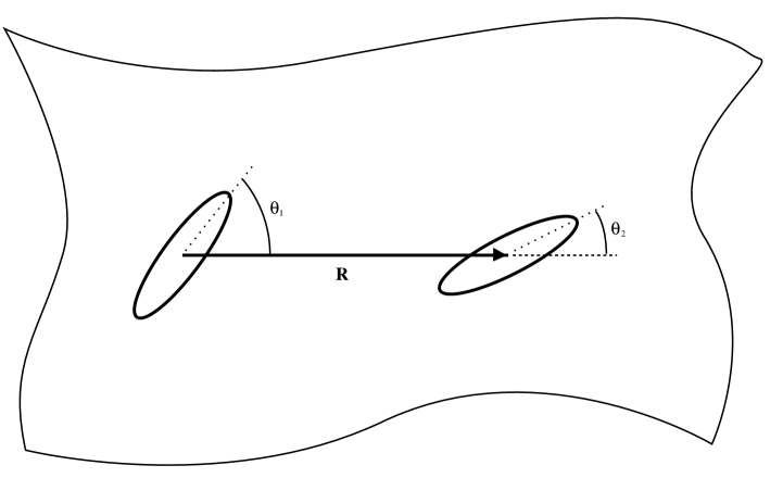
FIG. 1.: Proteins make angles $\theta_{i}$ measured with respect to the separation vector ${\bf R}$. The distance between proteins $R$ is taken to be much larger than protein size.

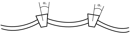
FIG. 2.: Contact angle $\alpha_{i}$ is measured between the direction of $i$-th protein and the unit normal of the membrane at protein’s perimeter.

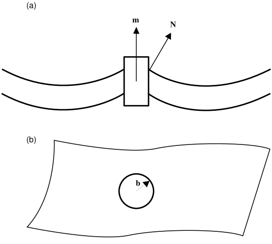
FIG. 3.: (a) The unit vector ${\bf m}$ denotes the direction of the protein and ${\bf N}$ denotes the unit normal vector of the membrane at the perimeter of protein (Side view). (b) ${\bf b}$ is the unit vector from the center of the protein to its perimeter (Top view).

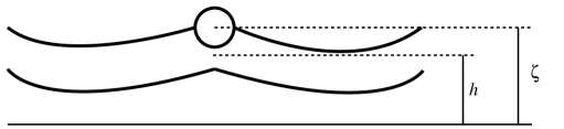
FIG. 4.: Non-transmembrane proteins have preferred center-of-mass positions nat at the center of the bilayer. $\zeta$ denotes the position of the protein and $h$ is the membrane height fluctuation field. The potential energy has a minimum at the non-vanishing value of $\zeta-h=r_{0}$.

REFERENCES

- [1] R.C. Warren, Physics and the Architecture of Cell Membranes, (Adam Hilger, Philadelphia, 1987).
- [2] D. Voet and J.G. Voet, Biochemistry, (Wiley, New York, 1990).
- [3] B. Alberts, J. Lewis, M. Raff, K. Roberts and J.D. Watson, Molecular Biology of the Cell, (Garland, New York, 1994).
- [4] R.B. Gennis, Biomembranes, Molecular structure and Function, (Springer-Verlag, New York, 1989).
- [5] C. Tanford, The Hydrophobic Effect: Formation of Micelles and Biological Membranes, (Wiley, New York, 1980).
- [6] J. Israelachvili, Intermolecular and Surface Forces, (Academic Press, San Diego, 1992).
- [7] M. Goulian, R. Bruinsma, and P. Pincus, Europhys. Lett. 22, 145 (1993); Erratum Europhys. Lett. 23, 155 (1993).
- [8] W. Helfrich, Z. Naturforsch 28C, 693 (1973).
- [9] P. Canham, J. Theo. Bio. 26, 61 (1970).
- [10] F. Brochard and J.F. Lennon, J. Phys. (Paris) 36, 1035 (1975).
- [11] F. David and S. Leibler, J. Phys. France II 1, 959 (1991).
- [12] R. Golestanian, M. Goulian, and M. Kardar, “Fluctuation-Induced Interactions between Rods on Membranes”, (preprint).
-
[13]
To calculate a cut-off for the height
fluctuation approximately, we use the fact that the number of points in the
first Brillouin zone is equal to the number of sites in the real space.
Since the height fluctuation is forbidden on scales less than the radius of
the proteins, we find
where is the linear size of the membrane. Thus, we obtain and this approximation is consistent with the ultra-violet regularization adapted in Ref. [7]. - [14] N. Dan, P. Pincus, and S.A. Safran, Langmuir 9, 2768 (1993).
- [15] N. Dan, A. Berman, P. Pincus, and S.A. Safran, J. Phys. France II 4, 1713 (1994).