Abstract

The Hubbard model is a “highly oversimplified model” for electrons in a solid which interact with each other through extremely short ranged repulsive (Coulomb) interaction. The Hamiltonian of the Hubbard model consists of two pieces; $H_{\rm hop}$ which describes quantum mechanical hopping of electrons, and $H_{\rm int}$ which describes nonlinear repulsive interaction. Either $H_{\rm hop}$ or $H_{\rm int}$ alone is easy to analyze, and does not favor any specific order. But their sum $H=H_{\rm hop}+H_{\rm int}$ is believed to exhibit various nontrivial phenomena including metal-insulator transition, antiferromagnetism, ferrimagnetism, ferromagnetism, Tomonaga-Luttinger liquid, and superconductivity. It is believed that we can find various interesting “universality classes” of strongly interacting electron systems by studying the idealized Hubbard model.

In the present article we review some mathematically rigorous results on the Hubbard model which shed light on “physics” of this fascinating model. We mainly concentrate on magnetic properties of the model at its ground states. We discuss Lieb-Mattis theorem on the absence of ferromagnetism in one dimension, Koma-Tasaki bounds on decay of correlations at finite temperatures in two-dimensions, Yamanaka-Oshikawa-Affleck theorem on low-lying excitations in one-dimension, Lieb’s important theorem for half-filled model on a bipartite lattice, Kubo-Kishi bounds on the charge and superconducting susceptibilities of half-filled models at finite temperatures, and three rigorous examples of saturated ferromagnetism due to Nagaoka, Mielke, and Tasaki. We have tried to make the article accessible to nonexperts by describing basic definitions and elementary materials in detail.

1 Introduction

According to the textbook of Ashcroft and Mermin, the Hubbard model is “a highly oversimplified model” for strongly interacting electrons in a solid. The Hubbard model is a kind of minimum model which takes into account quantum mechanical motion of electrons in a solid, and nonlinear repulsive interaction between electrons. There is little doubt that the model is too simple to describe actual solids faithfully.

Nevertheless, the Hubbard model is one of the most important models in theoretical physics. In spite of its simple definition, the Hubbard model is believed to exhibit various interesting phenomena including metal-insulator transition, antiferromagnetism, ferrimagnetism, ferromagnetism, Tomonaga-Luttinger liquid, and superconductivity. Serious theoretical studies have also revealed that to understand various properties of the Hubbard model is a very difficult problem. We believe that in course of getting deeper understanding of the Hubbard model, we will learn many new physical and mathematical techniques, concepts, and ways of thinking. Perhaps a more important point comes from the idea of “universality.” We believe that nontrivial phenomena and mechanisms found in the idealized Hubbard model can also be found in other systems in the same “universality class” as the idealized model. The universality class is expected to be large and rich enough so that it contains various realistic strongly interacting electron systems with complicated details which are ignored in the idealized model.

The situation is very similar to that of the Ising model for classical spin systems. The Ising model is too simple to be a realistic model of magnetic materials, but has turned out to be extremely important and useful in developing various notions and techniques in statistical physics of many degrees of freedom. Many important universality classes (of spin systems and field theories) were discovered by studying the Ising model.

In the present article, we review some mathematically rigorous results known for the Hubbard model. We shall concentrate ourselves mainly on magnetic properties of the model at its ground state, i.e., at the zero temperature. We have also decided not to cover many important rigorous and/or exact results in one-dimensional models based on the Bethe ansatz solutions. Even with these restrictions, we do not try to cover all the existing rigorous results. We recall that there is an excellent review article by Lieb [1] which covers wider topics than we do here. As for the more restricted topics of Nagaoka’s ferromagnetism, flat-band ferromagnetism, and some related topics, there is a separate review [2] which is more detailed and elementary than the present one.

2 Hubbard Model

2.1 Definition of the Hubbard Model

We first give general definition of the Hubbard model. Let the lattice $\Lambda$ be a collection of sites $x,y,\ldots$. Physically speaking, each lattice site corresponds to an atomic site in a crystal. In the standard Hubbard model, one simplifies the situation considerably, and assumes that each atom has only one electron orbit and the corresponding orbital state is non-degenerate. Of course actual atoms can have more then one orbits (or bands) and electrons in the corresponding states. The philosophy behind the model building is that those electrons in other states do not play significant roles in low-energy physics that we are interested in, and can be “forgotten” for the moment. See Figure 1.

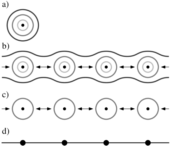
Figure 1: A highly schematic figure which explain philosophy of tight-binding descriptions. a) A single atom with multiple electrons in different orbits. b) When atoms get together to form a solid, electrons in the black orbits become itinerant, while those in the light gray orbits are still localized at the original atomic sites. Electrons in the gray orbits are mostly localized around the atomic sites, but tunnel to nearby gray orbits with a non-negligible probabilities. c) We only consider the electrons in the gray orbits, which are expected to play essential roles in determining various low energy physics of the system. d) If the gray orbit is non-degenerate, we get a lattice model in which electrons live on lattice sites and hop from site to another.

By $c^{\dagger}_{x,\sigma}$, we denote the operator which creates an electron with spin $\sigma=\uparrow,\downarrow$ at site $x\in\Lambda$. The corresponding annihilation operator is $c_{x,\sigma}$, and $n_{x,\sigma}=c^{\dagger}_{x,\sigma}c_{x,\sigma}$ is the number operator. These fermion operators obey the canonical anticommutation relations

$$\left\{c^{\dagger}_{x,\sigma},c_{y,\tau}\right\}=\delta_{x,y}\delta_{\sigma,\tau},$$ (2.1)

and

$$\left\{c^{\dagger}_{x,\sigma},c^{\dagger}_{y,\tau}\right\}=\left\{c_{x,\sigma},c_{y,\tau}\right\}=0,$$ (2.2)

where $\left\{A,B\right\}=AB+BA$.

By $\Phi_{\rm vac}$ we denote the state without any electrons. We have $c_{x,\sigma}\Phi_{\rm vac}=0$ for any $x\in\Lambda$ and $\sigma=\uparrow,\downarrow$. The Hilbert space of the model is generated by the states obtained by successively operating the creation operator $c^{\dagger}_{x,\sigma}$ with various $x$ and $\sigma$ onto the state $\Phi_{\rm vac}$. Since the anticommutation relation (2.2) implies $(c^{\dagger}_{x,\sigma})^{2}=0$, each lattice site can either be vacant, occupied by an $\uparrow$ or $\downarrow$ electron, or occupied by both $\uparrow$ and $\downarrow$ electrons. The total dimension of the Hilbert space is thus $4^{|\Lambda|}$.

The Hamiltonian of the Hubbard model is most naturally represented as the sum of two terms as

$$H=H_{\rm hop}+H_{\rm int}.$$ (2.3)

The most general form of the hopping Hamiltonian $H_{\rm hop}$ is

$$H_{\rm hop}=\sum_{x,y\in\Lambda}\sum_{\sigma=\uparrow,\downarrow}t_{x,y}\,c^{\dagger}_{x,\sigma}c_{y,\sigma}.$$ (2.4)

The hopping amplitude $t_{x,y}=t_{y,x}$, which is assumed to be real, represents the quantum mechanical amplitude that an electron hops from site $x$ to $y$ (or from $y$ to $x$). When $x=y$, the summand in (2.4) becomes $t_{x,x}\,c^{\dagger}_{x,\sigma}c_{x,\sigma}=t_{x,x}\,n_{x,\sigma}$, which is nothing but a single-body potential.

The interaction Hamiltonian $H_{\rm int}$ is written as

$$H_{\rm int}=\sum_{x\in\Lambda}U_{x}\,n_{x,\uparrow}n_{x,\downarrow},$$ (2.5)

where $U_{x}>0$ is a constant. The Hamiltonian represents a nonlinear interaction which raises the energy by $U_{x}$ when two electrons occupy a single orbital state at $x$. Although the original Coulomb interaction is long ranged, we have “oversimplified” the situation and took into account the strongest part out of the interaction. Another interpretation is that the Coulomb interaction is screened by the electrons in different orbital states which we had decided to forget.

2.2 Some Physical Quantities

We shall define some basic conserved quantities. The total number operator

$$\hat{N}_{\rm e}=\sum_{x\in\Lambda}(n_{x,\uparrow}+n_{x,\downarrow})$$ (2.6)

commutes with the Hamiltonian $H$. Although there are some conserved quantities other than $\hat{N}_{\rm e}$, one usually discusses stationary states or equilibrium states of the system by keeping the eigenvalue or the expectation value of $\hat{N}_{\rm e}$ constant. In the present article, we mostly consider the Hilbert space in which the number operator $\hat{N}_{\rm e}$ has a fixed eigenvalue $N_{\rm e}$. Since each lattice site can have at most two electrons, we have $0\leq N_{\rm e}\leq 2|\Lambda|$. The total electron number $N_{\rm e}$ is the most fundamental parameter in the Hubbard model.

The spin operator $\hat{\bf S}_{x}=(\hat{S}^{(1)}_{x},\hat{S}^{(2)}_{x},\hat{S}^{(3)}_{x})$ at site $x$ is defined as

$$\hat{S}^{(\alpha)}_{x}=\frac{1}{2}\sum_{\sigma,\tau=\uparrow,\downarrow}c^{\dagger}_{x,\sigma}(p^{(\alpha)})_{\sigma,\tau}\,c_{x,\sigma},$$ (2.7)

for $\alpha=1,2$, and $3$, where $p^{(\alpha)}$ are the Pauli matrices. The operators for the total spin of the system are defined as

$$\hat{S}^{(\alpha)}_{\rm tot}=\sum_{x\in\Lambda}\hat{S}^{(\alpha)}_{x},$$ (2.8)

for $\alpha=1,2$, and $3$. The operator $\hat{S}^{(\alpha)}_{\rm tot}$ commute with both the hopping Hamiltonian $H_{\rm hop}$ (2.4) and with the interaction Hamiltonian $H_{\rm int}$ (2.5). In other words, these Hamiltonians are invariant under any global rotation in the spin space.

As the operators $\hat{S}^{(\alpha)}_{\rm tot}$ with $\alpha=1,2,3$ do not commute with each other, we follow the convention in the theory of angular momenta, and simultaneously diagonalize the total spin operators $\hat{S}^{(3)}_{\rm tot}$, $(\hat{\bf S}_{\rm tot})^{2}=\sum_{\alpha=1}^{3}(\hat{S}^{(\alpha)}_{\rm tot})^{2}$, and the Hamiltonian $H$. We denote by $S_{\rm tot}^{(3)}$ and $S_{\rm tot}(S_{\rm tot}+1)$ the eigenvalues of $\hat{S}^{(3)}_{\rm tot}$ and $(\hat{\bf S}_{\rm tot})^{2}$, respectively. For a given electron number $N_{\rm e}$, we let

$$S_{\rm max}=\cases{N_{\rm e}/2&when $0\leq N_{\rm e}\leq|\Lambda|$;\cr|\Lambda|-(N_{\rm e}/2)&when $|\Lambda|\leq N_{\rm e}\leq 2|\Lambda|$.\cr}$$ (2.9)

Then the possible values of $S_{\rm tot}$ are $S_{\rm tot}=0,1,\ldots,S_{\rm max}$ (or $S_{\rm tot}=1/2,3/2,\ldots,S_{\rm max}$).

When we discuss magnetism of the system, the most important issue is to determine the value of $S_{\rm tot}$ in the ground state(s). If the total spin of the ground state grows proportionally to the number of sites $|\Lambda|$ as we increase the size of $\Lambda$, we say that the system exhibits ferromagnetism in a broad sense. This roughly means that the system behaves as a “magnet.” If the total spin of the ground state(s) coincides with the maximum possible value $S_{\rm max}$, we say that the system exhibits saturated ferromagnetism.

The following quantity will be useful in the later analysis.

Definition 2.1 (The lowest energy for each $S_{\rm tot}$)

Fix the electron number $N_{\rm e}$. For $S=0,1,\ldots,S_{\rm max}$ (or $S=1/2,3/2,\ldots,S_{\rm max}$), we denote by $E_{\rm min}(S)$ the lowest possible energy among the states which satisfy $\hat{N}_{\rm e}\Phi=N_{\rm e}\Phi$ and $(\hat{\bf S}_{\rm tot})^{2}\Phi=S(S+1)\Phi$ (i.e., $S_{\rm tot}=S$).

The appearance of saturated ferromagnetism is equivalent to have $E_{\rm min}(S)>E_{\rm min}(S_{\rm max})$ for any $S$ such that $S<S_{\rm max}$.

3 Basic Facts about the Model

In order to understand the meaning of the Hamiltonian of the Hubbard model, we discuss physics we encounter in two limiting situations.

3.1 Non-Interacting System

Let us assume that the Coulomb interaction in $H_{\rm int}$ (2.5) satisfies $U_{x}=0$ for any $x\in\Lambda$. Since the remaining Hamiltonian $H=H_{\rm hop}$ (2.4) is a quadratic form in fermion operators, it can be diagonalized easily (in principle). The single-electron Schrödinger equation corresponding to the hopping Hamiltonian $H_{\rm hop}$ (2.4) is

$$\sum_{y\in\Lambda}t_{x,y}\,\varphi_{y}=\varepsilon\varphi_{x},$$ (3.1)

where $\boldsymbol{\varphi}=(\varphi_{x})_{x\in\Lambda}$ is a single-electron wave function, and $\varepsilon$ is the single-electron energy eigenvalue. We shall denote the eigenvalues and the eigenstates of (3.1) as $\varepsilon_{j}$ and $\boldsymbol{\varphi}^{(j)}=(\varphi^{(j)}_{x})_{x\in\Lambda}$, respectively, where the index takes values $j=1,2,\ldots,|\Lambda|$. We count the energy levels with taking degeneracies into account, and order them as $\varepsilon_{j}\leq\varepsilon_{j+1}$.

Let us discuss a simple and standard example. Take a one dimensional lattice $\Lambda=\left\{1,2,\ldots,N\right\}$, and impose a periodic boundary condition which identifies the site $1$ with the site $N+1$. As for the hopping matrix elements, we set $t_{x,x+1}=t_{x+1,x}=-t$, and $t_{x,y}=0$ otherwise. The corresponding Schrödinger equation (3.1) can be solved easily. By using the wave number $k=2\pi n/N$ (with $n=0,\pm 1,\pm 2,\ldots,\pm\left\{(N/2)-1\right\},N/2$), the eigenstates and the eigenvalues can be written as $N^{-1/2}\exp[ikx]$ and $\varepsilon(k)=-2t\cos k$, respectively. If one makes a suitable correspondence between $n$ and $j=1,2,\ldots,N$, we get the desired energy level $\varepsilon_{j}$.

We return to the general setting, and define fermion operators corresponding to the eigenstates $\boldsymbol{\varphi}^{(j)}=(\varphi^{(j)}_{x})_{x\in\Lambda}$ by

$$a^{\dagger}_{j,\sigma}=\sum_{x\in\Lambda}\varphi^{(j)}_{x}c^{\dagger}_{x,\sigma}.$$ (3.2)

By using the orthonormality of the set of eigenstates $(\boldsymbol{\varphi}^{(j)})_{j=1,2,\ldots,|\Lambda|}$ (we redefine the eigenstates if they do not form an orthonormal set), one finds that the inverse transformation of (3.2) is $c_{x,\sigma}=\sum_{j=1}^{|\Lambda|}\varphi^{(j)}_{x}a_{j,\sigma}$. Substituting this into (2.4), and by using (3.1), we find that $H_{\rm hop}$ can be diagonalized as

$$H_{\rm hop}=\sum_{\sigma=\uparrow,\downarrow}\sum_{j=1}^{|\Lambda|}\varepsilon_{j}\,a^{\dagger}_{j,\sigma}a_{j,\sigma}=\sum_{\sigma=\uparrow,\downarrow}\sum_{j=1}^{|\Lambda|}\varepsilon_{j}\,\tilde{n}_{j,\sigma}.$$ (3.3)

Here $\tilde{n}_{j,\sigma}=a^{\dagger}_{j,\sigma}a_{j,\sigma}$ can be interpreted as the electron number operator for the $j$-th single-electron eigenstate.

Let $A,B$ be two arbitrary subsets of $\left\{1,2,\ldots,|\Lambda|\right\}$ which satisfy $|A|+|B|=N_{\rm e}$. By using (3.3), we find that the state

$$\Phi_{A,B}=\left(\prod_{j\in A}a^{\dagger}_{j,\uparrow}\right)\left(\prod_{j\in B}a^{\dagger}_{j,\downarrow}\right)\Phi_{\rm vac}$$ (3.4)

is an eigenstate of $H=H_{\rm hop}$ and its energy eigenvalue is

$$E_{A,B}=\sum_{j\in A}\varepsilon_{j}+\sum_{j\in B}\varepsilon_{j}.$$ (3.5)

By choosing subsets $A,B$ which minimize $E_{A,B}$, we get ground state(s) of the non-interacting model.

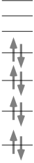
Figure 2: Schematic picture of the ground state of a non-interacting many electron system. The lowest $N_{\rm e}/2$ single-electron energy levels are “filled” by both up spin and down spin electrons. The state naturally exhibits paramagnetism known as Pauli paramagnetism.

In particular if the corresponding single-electron energy eigenvalues are nondegenerate, i.e., $\varepsilon_{j}<\varepsilon_{j+1}$, and $N_{\rm e}$ is even, the ground state of $H=H_{\rm hop}$ is unique and written as

$$\Phi_{\rm GS}=\left(\prod_{j=1}^{N_{\rm e}/2}a^{\dagger}_{j,\uparrow}a^{\dagger}_{j,\downarrow}\right)\Phi_{\rm vac}.$$ (3.6)

This is nothing but the state obtained by “filling up” the low energy levels by up and down spin electrons, as one learns in elementary quantum mechanics (Figure 2). It is easily verified that the above state has a definite total spin $S_{\rm tot}=0$. The ground state (3.6) exhibits no long range order. A system with no magnetic ordering is usually said to exhibit paramagnetism.

In the simple example in one dimension, all the energy levels except $\varepsilon(0)=-2t$ and $\varepsilon(\pi)=2t$ are two-fold degenerate. In this case the ground state of $H=H_{\rm hop}$ may not be unique for some values of $N_{\rm e}$. However the degeneracy of the ground states is at most four-fold, and the total spin of the ground states can take values in $S_{\rm tot}=0,1/2$, or $1$. We can conclude that the property of the ground state(s) is essentially the same as the models without degeneracy. In general we can draw the same conclusion unless the single-electron spectrum has a bulk degeneracy.

In a single-electron eigenstate of the example in one dimension, the electron is in a plane wave state with a definite wave number $k$. The fact that the Hamiltonian $H=H_{\rm hop}$ is diagonalized as (3.3) implies that the electrons behave as “waves” in this non-interacting (Hubbard) model. The same comment applies to any translation invariant (Hubbard) model with $U_{x}=0$.

3.2 Non-Hopping System

Let us next assume that the hopping matrix elements in $H_{\rm hop}$ (2.4) satisfy $t_{x,y}=0$ for any $x,y\in\Lambda$. Then the remaining Hamiltonian $H=H_{\rm int}$ (2.5) is already in a diagonal form. A general eigenstate can be written as

$$\Psi_{X,Y}=\left(\prod_{x\in X}c^{\dagger}_{x,\uparrow}\right)\left(\prod_{x\in Y}c^{\dagger}_{x,\downarrow}\right)\Phi_{\rm vac}.$$ (3.7)

Here $X$ and $Y$ are arbitrary subsets of $\Lambda$, and represent lattice sites which are occupied by up-spin electrons and down-spin electrons, respectively. The total electron number in this state is $N_{\rm e}=|X|+|Y|$, and the energy eigenvalue is given by

$$E_{X,Y}=\sum_{x\in X\cap Y}U_{x}.$$ (3.8)

The ground state for a given electron number $N_{\rm e}$ can be constructed by choosing subsets $X,Y$ that minimize the energy $E_{X,Y}$. When one has $N_{\rm e}\leq|\Lambda|$, one can always choose $X$ and $Y$ such that $X\cap Y=\emptyset$. Thus the ground state has energy equal to $0$.

The ground states of the non-hopping Hubbard model has no magnetic long range order. Again the system is paramagnetic. It is also clear (from the beginning) that the electrons behave as “particles” in non-hopping models.

3.3 Hubbard Model is Difficult, but it is Interesting

We have investigated the properties of the two pieces $H_{\rm hop}$ and $H_{\rm int}$ in the Hubbard Hamiltonian. It turned out that both $H_{\rm hop}$ and $H_{\rm int}$ are easy to analyze. We also found that neither of them favor any magnetic ordering.

We also observed, however, that electrons behave as “waves” in $H_{\rm hop}$, while they behave as “particles” in $H_{\rm int}$. How do they behave in a system with the Hamiltonian which is a sum of these totally different Hamiltonians? This is indeed a fascinating problem which is deeply related to the wave-particle dualism in quantum physics. We might say that many of the important models in many-body problems, including the $\varphi^{4}$ quantum field theory and the Kondo problem, are minimum models which take into account at the same time the wave-like nature and the particle-like nature (through point-like nonlinear interaction) of matter.

From a technical point of view, the wave-particle dualism implies that the Hamiltonians $H_{\rm int}$ are $H_{\rm hop}$ do not commute with each other. Even when each Hamiltonian is diagonalized, it is still highly nontrivial (or impossible) to find the properties of their sum. Of course mathematical difficulty does not automatically guarantee that the model is worth studying. A really exciting thing about the Hubbard model is that, though the Hamiltonians $H_{\rm hop}$ and $H_{\rm int}$ do not favor any nontrivial order, their sum $H=H_{\rm hop}+H_{\rm int}$ is believed to generate various nontrivial order including antiferromagnetism, ferromagnetism, and superconductivity. When we sum up the two innocent Hamiltonians $H_{\rm hop}$ and $H_{\rm int}$, competition between wave-like character and particle-like character (or between linearity and nonlinearity) takes place, and one gets various interesting “physics.” To confirm this fascinating scenario is a very challenging problem to theoretical and mathematical physicists.

4 Results for Low Dimensional Models

We discuss some theorems which are proved by using special natures of low-dimensional systems.

4.1 Lieb-Mattis Theorem

Theorems discussed in the present and the next sections state that the Hubbard model does not exhibit interesting long range order under some conditions. The main purpose of studying an idealized model like the Hubbard model should be to show that some interesting physics do take place. Results which say something does not take place may be regarded as less exciting. But to have a definite knowledge that something does not happen under some conditions is very useful and important even if our final goal is to show something does happen.

The classical Lieb-Mattis theorem [7] states (among other things) that one can never have ferromagnetism in one-dimensional Hubbard model with only nearest neighbor hoppings.

Theorem 4.1 (Lieb-Mattis theorem)

Consider a Hubbard model on a one-dimensional lattice $\Lambda=\left\{1,2,\ldots,N\right\}$ with open boundary conditions. We assume that the hopping matrix elements satisfy $|t_{x,y}|<\infty$ when $x=y$, $0<|t_{x,y}|<\infty$ when $|x-y|=1$, and are vanishing otherwise. We also assume $|U_{x}|<\infty$ for any $x\in\Lambda$. Then the quantity $E_{\rm min}(S)$ (see Definition 2.1) satisfies the inequality

$$E_{\rm min}(S)<E_{\rm min}(S+1),$$ (4.1)

for any $S=0,1,\ldots,S_{\rm max}-1$ (or $S=1/2,3/2,\ldots,S_{\rm max}-1$).

One of the most important consequences of the Lieb-Mattis theorem is that any one-dimensional Hubbard model in the above class has the total spin $S_{\rm tot}=0$ (or $S_{\rm tot}=1/2$) in its ground state. One cannot conclude from this fact alone that the system exhibits paramagnetism, but can conclude that there is no ferromagnetism.

Theorem 4.1 does not apply to models with periodic boundary conditions. But it seems reasonable that boundary conditions do not change the essential physics provided that the system is sufficiently large. If there exist hoppings to sites further than the nearest neighbor, on the other hand, the story is totally different. We do not only find that the proof of Theorem 4.1 fails, but we also find essentially new physics. See Section 6.5.

Theorem 4.1 is proved by noting that, in a suitable basis, the Hamiltonian is written as a matrix whose nondiagonal elements are nonpositive, and by using the standard Perron-Frobenius argument. Similar argument was used by Lieb and Mattis in their study of the Heisenberg quantum spin system [8].

4.2 Decay of Correlations at Finite Temperatures

Among other rigorous results which show the absence of order is the extension by Ghosh [9] of the wellknown theorem of Mermin and Wagner. Ghosh proved that the Hubbard model in one- or two-dimensions does not exhibit symmetry breaking related to magnetic long range order at any finite temperatures. By using the same method, one can also prove the absence of superconducting $U(1)$ symmetry breaking.

Koma and Tasaki proved essentially the same facts in terms of explicit upper bounds for various correlation functions [10]. Among the results of [10] is the following.

Theorem 4.2 (Koma-Tasaki bounds for correlations)

Consider an arbitrary Hubbard model in one- or two-dimensions with finite range hoppings. Then there are constants $\alpha,\gamma$, and we have

$$\left|\left\langle c^{\dagger}_{x,\uparrow}c^{\dagger}_{x,\downarrow}c_{y,\uparrow}c_{y,\downarrow}+\mbox{\em H.c.}\right\rangle_{\beta}\right|\leq\cases{|x-y|^{-\alpha f(\beta)}&\em in $d=2$;\cr\exp[-\gamma f(\beta)|x-y|]&\em in $d=1$,}$$ (4.2)

and

$$\left|\left\langle{\bf S}_{x}\cdot{\bf S}_{y}\right\rangle_{\beta}\right|\leq\cases{|x-y|^{-\alpha f(\beta)}&\em in $d=2$;\cr\exp[-\gamma f(\beta)|x-y|]&\em in $d=1$,}$$ (4.3)

for sufficiently large $|x-y|$, where $\left\langle\cdots\right\rangle_{\beta}$ denotes the canonical average in the thermodynamic limit at the inverse temperature $\beta$. Here $f(\beta)$ is a decreasing function of $\beta$ and behaves as $f(\beta)\approx 1/\beta$ for $\beta\gg\delta$ and $f(\beta)\approx(2/\delta)|\ln\beta|$ for $\beta\ll\delta$, where $\delta$ is a constant.

The bounds (4.2) and (4.3) establishes the widely accepted fact that there can be no superconducting or magnetic long-range order at finite temperatures in one- or two-dimensions. The method employed in [10], i.e., a combination of the McBryant-Spencer method and the quantum mechanical global $U(1)$ gauge invariance, is rather interesting. It is amusing that only by using the $U(1)$ symmetry which exists in any quantum mechanical system, one gets upper bounds for correlations which are almost optimal at low temperatures (especially in one-dimension).

4.3 Yamanaka-Oshikawa-Affleck Theorem

We discuss a recent important theorem by Yamanaka, Oshikawa, and Affleck [11, 12] about low-lying excitations in general electron systems on a one-dimensional lattice. The theorem is an extension of Lieb-Schultz-Mattis theorem for quantum spin chains. It can also be interpreted as a nonperturbative version of Luttinger’s “theorem” restricted to one-dimension.

We consider the Hubbard model on the one-dimensional lattice $\Lambda=\{1,2,\ldots,N\}$ with periodic boundary conditions. The model is characterized by positive integers $R$ and $P$, which are the range of hopping and the period of the system, respectively. We assume $t_{x,y}=0$ whenever $|x-y|>R$, and $t_{x+P,y+P}=t_{x,y}$, $U_{x+P}=U_{x}$ for any $x,y\in\Lambda$. Under this general assumption, we have the following.

Theorem 4.3 (Yamanaka-Oshikawa-Affleck theorem)

Consider the infinite volume limit $N\to\infty$ with a fixed electron density $\nu=N_{\rm e}/N$. If $P\nu/2$ is not an integer, then we have one of the following two possibilities.

i) There is a symmetry breaking, and the infinite volume ground states are not unique.

ii) There is a gapless excitation above the infinite volume ground state.

In other words, the theorem rules out the third possibility;

iii) The infinite volume ground state is unique, and there is a finite gap above it.

Note that iii) does take place if $P\nu/2$ is an integer and the system describes an innocent insulator. In a non-interacting system, it is evident that iii) is impossible when $P\nu/2$ is not an integer, since there is a partially filled band. The above theorem guarantees that we cannot change the situation by introducing strong interaction. This is of course far from obvious.

The proof of Theorem 4.3 is based on the following explicit construction of a (trial) low-lying excitation. Consider a system on a periodic chain of length $N$, and assume that the ground state $\Phi_{\rm GS}$ is unique. We define the “twist” operator by $U=\exp[2\pi i\sum_{x=1}^{N}(x/N)n_{x,\uparrow}]$ which introduces a gradual twist in the $U(1)$ phase of the up-spin electron field, and consider the trial excited state $\Psi=U\Phi_{\rm GS}$. It is not hard to show that $\left\langle\Psi,H\Psi\right\rangle-E_{\rm GS}=O(1/L)$. Thus $\Psi$ contains a low-lying excited state provided it is orthogonal to the ground state. To see the orthogonality, let $T_{P}$ be the translation by $P$, and assume that the ground state is chosen as $T_{P}\Phi_{\rm GS}=\Phi_{\rm GS}$. It is easily found that $T_{P}\Psi=e^{i\pi P\nu}\Psi$, and hence the trial state $\Psi$ is orthogonal to $\Phi_{\rm GS}$ whenever $P\nu/2$ is not an integer.

The above result also implies that, in the case ii), the gapless excitation $\Psi$ has a crystal momentum $k_{\Psi}=\pi\nu$. If we interpret this excitation as obtained from the ground state by moving an electron at a “fermi point” to the other fermi point, we find that the fermi momentum $k_{\rm F}$ satisfies $k_{\Psi}=2k_{\rm F}$, and hence $k_{\rm F}=\pi\nu/2$. This is nothing but the fermi momentum of the free system. Therefore the fermi momentum is not “renormalized” by strong interaction among electrons. As far as we know, this is the only general rigorous result which gives precise meaning to fermi momentum in truly interacting many electron systems.

5 Half-Filled Systems

A system in which the electron number $N_{\rm e}$ is identical to the number of sites $|\Lambda|$ is said to be half-filled, since the maximum possible value of $N_{\rm e}$ is $2|\Lambda|$. The system becomes half-filled if each atom provides one electron to the system. Thus the half-filled models represent physically natural situations. Half-filled models have nice properties from mathematical point of view as well, and there are some very nice rigorous results.

5.1 Perturbation for $U\gg t$

Let us first look at the ground states of the non-hopping model with $H_{\rm hop}=0$. We here assume that $U_{x}>0$ for any $x\in\Lambda$. As we found in Section 3.2, one can choose $X\cap Y=\emptyset$ in the state $\Psi_{X,Y}$ to get a ground state with $E_{X,Y}=0$, provided that $N_{\rm e}\leq|\Lambda|$. Since we have $N_{\rm e}=|\Lambda|$, the assumption $X\cap Y=\emptyset$ automatically implies $X\cup Y=\Lambda$. Therefore the ground state $\Psi_{X,Y}$ (3.7) with $X\cap Y=\emptyset$ can be written also as

$$\Psi_{\boldsymbol{\sigma}}=\left(\prod_{x\in\Lambda}c^{\dagger}_{x,\sigma(x)}\right)\Phi_{\rm vac},$$ (5.1)

where $\boldsymbol{\sigma}=(\sigma(x))_{x\in\Lambda}$ is a collection of spin indices $\sigma(x)=\uparrow,\downarrow$. By using the terminology of spin systems, one can call $\boldsymbol{\sigma}$ a spin configuration. One can say that the degeneracy of the ground states (5.1) precisely corresponds to all the possible spin configurations.

Let us take into account effects of nonvanishing $H_{\rm hop}$ by using a simple-minded perturbation theory. As the diagonal elements of $H_{\rm hop}$, i.e., $\sum_{x,\sigma}t_{x,x}\,c^{\dagger}_{x,\sigma}c_{x,\sigma}=\sum_{x}t_{x,x}(n_{x,\uparrow}+n_{x,\downarrow})$, only shift the energy of the states $\Psi_{\boldsymbol{\sigma}}$ by a constant amount (independent of $\boldsymbol{\sigma}$), they can be omitted in the lowest order perturbation calculation. Let us denote by $\widetilde{H}_{\rm hop}=\sum_{x\neq y,\sigma}t_{x,y}\,c^{\dagger}_{x,\sigma}c_{y,\sigma}$ the off-diagonal part of $H_{\rm hop}$. By operating $\widetilde{H}_{\rm hop}$ once onto $\Psi_{\boldsymbol{\sigma}}$, an electron moves, and we get a state with one vacant site and one doubly occupied site. The resulting state is not a ground state of $H_{\rm int}$. We thus find that the lowest order contribution from this perturbation theory comes from the second order.

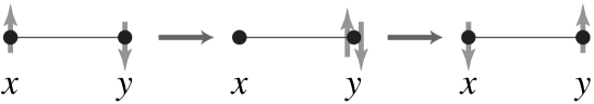
Figure 3: When electrons hop twice, spins on sites $x$ and $y$ may be exchanged. This is the ultimate origin of antiferromagnetic nature in the half-filled Hubbard model.

Figure 3 shows a process that is taken into account in the second order perturbation theory. The electron at site $x$ hops to site $y$ with the transition amplitude $t_{x,y}$, and generates a new state with extra energy $U_{y}$. Then one of the two electrons at site $y$ will hop back to site $x$, and we recover one of the ground states. In this process, spins at the sites $x$ and $y$ may be exchanged as Figure 3 shows. The hopping between sites $x$ and $y$ is inhibited by the Pauli principle if the electronic spins on these two sites are pointing in the same direction. We find that this second order perturbation process lowers the energy of states in which the spins at sites $x$ and $y$ are not pointing in the same direction (or more precisely, the states in which the total spin is vanishing).

Let us rederive this result in a more formal manner. Let $P_{0}$ be the projection operator onto the subspace spanned by the states $\Psi_{\boldsymbol{\sigma}}$ (5.1) with all the possible $\boldsymbol{\sigma}$. That the first order perturbation has no contribution can be read off from the fact that $P_{0}\widetilde{H}_{\rm hop}P_{0}=0$. To find out how the degeneracy in the (unperturbed) ground states (5.1) is lifted can be determined by the effective Hamiltonian

$$H_{\rm eff} = -P_{0}\widetilde{H}_{\rm hop}\frac{1}{H_{\rm int}}\widetilde{H}_{\rm hop}P_{0}$$ (5.2)

$$= P_{0}\left\{\sum_{x,y\in\Lambda}J_{x,y}\left(\hat{\bf S}_{x}\cdot\hat{\bf S}_{y}-\frac{1}{4}\right)\right\}P_{0}.$$

Here the exchange interaction parameter is given by $J_{x,y}=\{(t_{x,y})^{2}/U_{x}\}+\{(t_{x,y})^{2}/U_{y}\}$. Note that (5.2) is nothing but the Hamiltonian of the $S=1/2$ antiferromagnetic quantum Heisenberg spin system. This suggests that the low-energy behavior of the half-filled Hubbard model is well described by the Heisenberg antiferromagnets when $U_{x}$ are much larger than $t_{x,y}$.

5.2 Lieb’s Theorem

In 1989, Lieb proved an important and fundamental theorem for the half-filled Hubbard model. The theorem provides, among other things, partial support to the conjecture about the similarity of the half-filled Hubbard model and the Heisenberg antiferromagnets. Let us first introduce the notion of bipartiteness.

Definition 5.1 (Bipartiteness)

Consider a Hubbard model (or other tight-binding electron model) on a lattice $\Lambda$ with hopping matrix elements $\left(t_{x,y}\right)_{x,y\in\Lambda}$. The system is said to be bipartite if the lattice $\Lambda$ can be decomposed into a disjoint union of two sublattices as $\Lambda=A\cup B$ (with $A\cap B=\emptyset$), and it holds that $t_{x,y}=0$ whenever $x,y\in A$ or $x,y\in B$. In other words, only hoppings between different sublattices are allowed.

Then Lieb’s theorem [13] for the repulsive Hubbard model is as follows.

Theorem 5.2 (Lieb’s theorem)

Consider a bipartite Hubbard model. We assume $|\Lambda|$ is even, and the whole $\Lambda$ is connected through nonvanishing $t_{x,y}$. We also assume $U_{x}=U>0$ for any $x\in\Lambda$. Then the ground states of the model are nondegenerate apart from the trivial spin degeneracy, and have total spin $S_{\rm tot}=\bigl{|}|A|-|B|\bigr{|}/2$.

The total spin $S_{\rm tot}$ of the ground state determined in the theorem is exactly the same as that of the ground state(s) of the corresponding Heisenberg antiferromagnet on the same lattice. In fact the conclusion of the theorem is quite similar to that of the Lieb-Mattis theorem [8] for Heisenberg antiferromagnets. However the straightforward Perron-Frobenius argument used in the proof of the latter theorem does not apply to the Hubbard model except in one dimension. (See 4.) This is not only a technical difficulty, but is a consequence of the important fact that quantum mechanical processes allowed in the Hubbard model are in general much richer and more complex than those in the Heisenberg model. Lieb’s proof is compactly presented in a Letter, but is deep and elegant. The proof again makes use of a kind of Perron-Frobenius argument, but is based on an interesting technique called spin-space reflection positivity.

Lieb’s theorem is valid for any value of Coulomb repulsion $U$, only provided that it is positive. It is quite likely that physical properties of the Hubbard model are drastically different in the weak coupling region with small $U$ and in the strong coupling region with large $U$. It is very surprising and interesting that a single proof of Lieb’s covers the whole range with $U>0$ and clarifies the basic properties of the ground states.

It should be noted, however, that the knowledge of the total spin of the ground states in finite volume does not necessarily determine the properties of the ground states in the corresponding infinite system. When two sublattices have the same number of sites as $|A|=|B|$, for example, one knows that finite volume ground state is unique and has $S_{\rm tot}=0$. Although one might well conclude that the system has no long range order in its ground states, this is not true. It is certainly possible that infinite volume ground states exhibit long range order and symmetry breaking (such as antiferromagnetism of superconductivity) even when finite volume ground state is unique and symmetric. (See, for example, [14].) By knowing any finite volume ground state has $S_{\rm tot}=0$, however, one can rule out the possibility of ferromagnetism.

By using Lieb’s results in [13], one gets some information about excited states. For example, by combining Theorem 1 in [13] with the method of [8], one can easily prove the inequality

$$E_{\rm min}(S)<E_{\rm min}(S+1)$$ (5.3)

for any $||A|-|B||/2\leq S\leq(|\Lambda|/2)-1$.

Another theorem which suggests the similarity between the half-filled Hubbard model and the Heisenberg antiferromagnets is the following, proved by Shen, Qiu, and Tian [15, 16] by extending Lieb’s method.

Theorem 5.3 (Explicit signs of correlations)

Assume the conditions for Theorem 19. If we denote by $\Phi_{\rm GS}$ the ground state of the model, we have the inequalities

$$\left\langle\Phi_{\rm GS},\hat{\bf S}_{x}\cdot\hat{\bf S}_{y}\,\Phi_{\rm GS}\right\rangle\cases{>0&when $x,y\in A$, or $x,y\in B$;\cr<0&when $x\in A,y\in B$, or $x\in B,y\in A$,\cr}$$ (5.4)

were $\left\langle\cdot,\cdot\right\rangle$ denotes the quantum mechanical inner product.

We see that spins on different sublattices have negative correlations, indicating antiferromagnetic tendency.

The $S=1/2$ Heisenberg antiferromagnet on the cubic lattice, for example, is proved to exhibit an antiferromagnetic long range order at sufficiently low temperatures or in the ground states [17, 18]. It is likely that the same statements hold for the half-filled Hubbard model with sufficiently large $U$. But, for the moment, there are no methods or ideas which are useful in proving the conjecture. To extend the powerful (but not very natural) method of [17, 18] based on the (spatial) reflection positivity seems hopeless.

In the Hubbard model and related models at half-filling, there have been proved several interesting general results. Among the recent examples are the uniform density theorem [19], the solution of the flux phase problem [20, 21], and the stability of the Peierls instability [22].

5.3 Lieb’s Ferrimagnetism

A very important corollary of Lieb’s theorem 19 is that the half-filled Hubbard models on asymmetric bipartite lattices universally exhibit a kind of ferromagnetism (in the broad sense), or more precisely, ferrimagnetism [13].

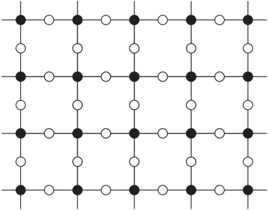
Figure 4: An example (the so called CuO lattice) of a bipartite lattice in which the number of sites in two sublattices are different. Lieb’s theorem implies that the half-filled Hubbard model defined on this lattice exhibits ferrimagnetism.

Take, for example, the so called CuO lattice in Figure 4. The lattice can be decomposed into two sublattices distinguished by black sites and white sites. When the black sites form a square lattice with side $L$, there are $L^{2}$ black sites and $2L^{2}$ white sites. We define the Hubbard model on this lattice, and put nonvanishing hopping $t_{x,y}$ on each bond in the lattice, and put Coulomb interaction $U>0$ on each site. Then Lieb’s theorem implies that the ground state of this Hubbard model has total spin $S_{\rm tot}=\bigl{|}|A|-|B|\bigr{|}/2=L^{2}/2$. Since the total spin magnetic moment of the system is proportional to the number of lattice sites $3L^{2}$, we conclude that the model exhibits ferromagnetism in the broad sense.

Of course the present ferromagnetism is not a saturated ferromagnetism in which all the spins in the system completely align with each other. As the inequality (5.4) suggests, spins on neighboring sites have tendency to point in the opposite direction. But the big difference in the numbers of sites in the sublattices cause the system to possess bulk magnetic moment. Such a magnetic ordering is usually called ferrimagnetism.

One can similarly construct Hubbard models which exhibit ferrimagnetism on any bipartite lattice in which the difference in the number of sites in two sublattices is proportional to the system size. The value of $U>0$ is again arbitrary, so Lieb’s ferrimagnetism covers surprisingly general class of models including weakly coupled ones as well as strongly coupled ones.

If one recalls the conclusion of Section 3.1 that systems with $U=0$ exhibit paramagnetism, one might feel it somehow contradicting that the above ferrimagnetism appears for arbitrarily small $U>0$. This is one of the special features of Lieb’s ferrimagnetism. In the single-electron Schrödinger equation corresponding the Hubbard model on Figure 4, for example, the eigenstates for the eigenvalue $\varepsilon=0$ are $L^{2}$-fold degenerate. (The eigenvalue $\varepsilon=0$ is at the middle of the single-electron spectrum.) Consequently the ground states of the half-filled ($N_{\rm e}=|\Lambda|=3L^{2}$) system with $U=0$ are highly degenerate, and the total spin can take values in $S_{\rm tot}=0,1,\ldots,L^{2}/2$. The role of Coulomb interaction $U$ is to lift this degeneracy, and select states with the largest magnetic moment as ground states.

5.4 Kubo-Kishi Bounds on Susceptibilities at Finite Temperatures

A theorem which can be regarded as a finite temperature version of Lieb’s theorem was proved by Kubo and Kishi [23]. It deals with the charge susceptibility and the on-site pairing (superconducting) susceptibility in a half-filled system at finite temperatures.

We define the thermodynamic function $J$ corresponding to the grand canonical ensemble by

$$J(\beta,\mu,(\gamma_{x})_{x\in\Lambda},(\eta_{x})_{x\in\Lambda})=$$

$$=-\frac{1}{\beta}\log{\rm Tr}\exp\left[-\beta\left(H-\mu\hat{N}_{\rm e}-\mathop{\sum_{x\in\Lambda}}_{\sigma=\uparrow,\downarrow}\gamma_{x}n_{x,\sigma}-\sum_{x\in\Lambda}\eta_{x}(c^{\dagger}_{x,\uparrow}c^{\dagger}_{x,\downarrow}+c_{x,\downarrow}c_{x,\uparrow})\right)\right],$$ (5.5)

where $\beta$ and $\mu$ are the inverse temperature and the chemical potential, respectively, and the trace is taken over the Hilbert spaces with all the possible electron numbers. We added to the Hamiltonian two fictitious external fields $(\gamma_{x})_{x\in\Lambda}$ and $(\eta_{x})_{x\in\Lambda}$ to test for the possible charge ordering and superconducting ordering, respectively.

We define the charge susceptibility $\chi^{\rm c}$ and the on-site pairing susceptibility $\chi^{\rm p}$ by

$$\chi^{\rm c}_{\bf q}(\beta,\mu)=-\left.\frac{\partial}{\partial\tilde{\gamma}_{\bf q}}\frac{\partial}{\partial\tilde{\gamma}_{-\bf q}}J(\beta,\mu,(\gamma_{x}),(\eta_{x}))\right|_{(\gamma_{x})=(\eta_{x})=0}\geq 0,$$ (5.6)

and

$$\chi^{\rm p}_{\bf q}(\beta,\mu)=-\left.\frac{\partial}{\partial\tilde{\eta}_{\bf q}}\frac{\partial}{\partial\tilde{\eta}_{-\bf q}}J(\beta,\mu,(\gamma_{x}),(\eta_{x}))\right|_{(\gamma_{x})=(\eta_{x})=0}\geq 0.$$ (5.7)

The Fourier transformation of the external fields are

$$\tilde{\gamma}_{\bf q}=|\Lambda|^{-1/2}\sum_{x\in\Lambda}\gamma_{x}\,e^{i{\bf q}\cdot x},\quad\tilde{\eta}_{\bf q}=|\Lambda|^{-1/2}\sum_{x\in\Lambda}\eta_{x}\,e^{i{\bf q}\cdot x},$$ (5.8)

where $\bf q$ is a wave vector corresponding to the lattice $\Lambda$ (which we assume to have a periodic structure).

Then the Kubo-Kishi theorem states that

Theorem 5.4

Consider any bipartite (see Definition 5.1) Hubbard model with $U_{x}=U>0$ for any $x\in\Lambda$. Then for any $\beta>0$ and for any wave vector $\bf q$, we have

$$\chi^{\rm c}_{\bf q}(\beta,U/2)\leq\frac{1}{U},\quad\mbox{\em and}\quad\chi^{\rm p}_{\bf q}(\beta,U/2)\leq\frac{2}{U}.$$ (5.9)

Note that the choice $\mu=U/2$ corresponds to the half-filling. The theorem states that the charge and the on-site paring susceptibilities for any wave vector $\bf q$ are finite in a half-filled model at finite temperatures. This means that the model does not exhibit any CDW ordering or superconducting ordering.

6 Ferromagnetism

Ferromagnetism, where almost all of the spins in the system align in the same direction, is a remarkable phenomenon. Standard theories about the origin of ferromagnetism have been the Heisenberg’s exchange interaction picture, and the Stoner criterion derived from the Hartree-Fock approximation for band electrons. But there have been serious doubts if these theories really explain the appearance of ferromagnetism in a system of electrons interacting via spin-independent Coulomb interaction. One of the motivations to study the Hubbard model was to understand the origin of ferromagnetism in an idealized situation.

As we have seen in the previous section, half-filled models have tendency towards antiferromagnetism. In this section we shall concentrate on systems in which the electron numbers deviate from half-filling.

6.1 Instability of Ferromagnetism

To see that ferromagnetism is indeed a delicate phenomenon, we discuss two elementary results which show that the Hubbard model with certain conditions does not exhibit ferromagnetism.

The following theorem states that there can be no saturated ferromagnetism if the Coulomb interaction $U$ is too small in a system with a “healthy” single-electron spectrum.

Theorem 6.1 (Impossibility of ferromagnetism for small $U$)

Let $\{\varepsilon_{j}\}_{j=1,\ldots,N}$ denote the single-electron energy eigenvalues with $\varepsilon_{j}\leq\varepsilon_{j+1}$ as in Section 3.1. If $0\leq U<\varepsilon_{N_{\rm e}}-\varepsilon_{1}$, we have

$$E_{\rm min}(S_{\rm max}-1)<E_{\rm min}(S_{\rm max}).$$ (6.1)

Thus the ground state of the model does not have $S_{\rm tot}=S_{\rm max}$.

When the density of electrons is very low, it is expected that the chance of electrons to collide with each other becomes very small. It is likely that the model is close to an ideal gas no matter how strong the interaction is, and there is no ferromagnetism.

This naive guess is easily justified for “healthy” models in dimensions three (or higher). The dimensionality of the lattice is taken into account by assuming that there are positive constants $c$, $\nu_{0}$, and $d$, and the single electron energy levels satisfy

$$\varepsilon_{n}-\varepsilon_{1}\geq c\left(\frac{n-1}{|\Lambda|}\right)^{2/d},$$ (6.2)

for any $n$ such that $n/|\Lambda|\leq\nu_{0}$. Note that the right-hand side represents the $n$ dependence of energy levels in an usual $d$-dimensional quantum mechanical system. Then we have the following theorem due to Pieri, Daul, Baeriswyl, Dzierzawa, and Fazekas [24].

Theorem 6.2 (Impossibility of ferromagnetism at low densities)

Suppose we have $H_{\rm hop}$ satisfying (6.2) with positive $c$, $\nu_{0}$, and $d>2$. Then there exists a constant $\nu_{1}>0$, and the same conclusion as Theorem 6.1 holds for any $U\geq 0$ if $N_{\rm e}/|\Lambda|\leq\nu_{1}$ holds.

That we have a restriction on dimensionality in Theorem 6.2 is not merely technical. In a one-dimensional system, moving electrons must eventually collide with each other for an obvious geometric reason. Thus a one-dimensional model cannot be regarded as close to ideal no matter how low the electron density is. We do not know whether the inapplicability of the theorem to $d=2$ systems is physically meaningful or not.

6.2 Toy Model with Two Electrons

As a starting point of our study of ferromagnetism, we consider a toy model with two electrons on a small lattice. Interestingly enough, some essential features of ferromagnetism found in many-electron systems (that we will discuss later in this section) are already present in the toy model.

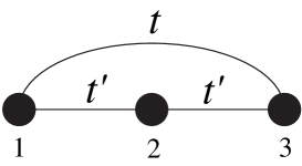
Figure 5: The lattice and the hopping of the toy model. By considering the system with two electrons on this lattice, we can observe some very important aspects of ferromagnetism in the Hubbard model.

The smallest possible model in which we can discuss electron interaction and which is away from half-filling is that with two electrons on a lattice with three sites. Consider the lattice $\Lambda=\left\{1,2,3\right\}$, and put one electron with $\sigma=\uparrow$ and one with $\sigma=\downarrow$. The hopping matrix is defined by $t_{1,2}=t_{2,3}=t^{\prime}$, and $t_{1,3}=t$. Note that there are two kinds of hoppings $t$ and $t^{\prime}$. Since the sign of $t^{\prime}$ can be changed by the gauge transformation $c_{2,\sigma}\to-c_{2,\sigma}$, we shall fix $t^{\prime}>0$. Figure 5 shows the lattice and the hopping. For simplicity, we assume there is only one kind of interaction, and set $U_{1}=U_{2}=U_{3}=U\geq 0$. We have $S_{\rm max}=1$ because $N_{\rm e}=2$. Therefore we can say that there appears saturated ferromagnetism if the ground state has $S_{\rm tot}=1$, i.e., if it is a part of a spin-triplet.

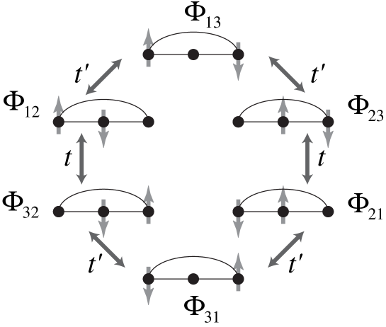
Figure 6: Allowed states and transition amplitudes in the toy model with $U=\infty$. The total spin of the ground states can be easily read off from this diagram.

Let us take the limit $U\to\infty$, in which the effect of interaction becomes most drastic, and consider only those states with finite energies. This is equivalent to consider only states in which two electrons never occupy a same site. There are six states which satisfy the constraint, and they can be written as $\Phi_{x,y}=c^{\dagger}_{x,\uparrow}c^{\dagger}_{y,\downarrow}\Phi_{\rm vac}$ where $x,y=1,2,3$, and $x\neq y$. Transition amplitudes between these states are shown in Figure 6. We find that the problem is equivalent to that of a quantum mechanical particle hopping around on a ring consisting of six sites. The basic structure of the ground state can be determined by the standard Perron-Frobenius sign convention. The ground state for $t<0$ is written as

$$\Phi_{\rm GS}^{(t<0)}=\Phi_{1,2}+\Phi_{3,2}-\alpha(t,t^{\prime})\Phi_{3,1}+\Phi_{2,1}+\Phi_{2,3}-\alpha(t,t^{\prime})\Phi_{1,3},$$ (6.3)

and that for $t>0$ as

$$\Phi_{\rm GS}^{(t>0)}=\Phi_{1,2}-\Phi_{3,2}+\beta(t,t^{\prime})\Phi_{3,1}-\Phi_{2,1}+\Phi_{2,3}-\beta(t,t^{\prime})\Phi_{1,3},$$ (6.4)

where $\alpha(t,t^{\prime})$ and $\beta(t,t^{\prime})$ are positive functions of $t$ and $t^{\prime}$.

To find the total spin of these states, it suffices to concentrate on two lattice sites, say sites 1 and 2, and note that $\Phi_{\rm GS}^{(t<0)}=\Phi_{1,2}+\Phi_{2,1}+\cdots$, and $\Phi_{\rm GS}^{(t>0)}=\Phi_{1,2}-\Phi_{2,1}+\cdots$. It immediately follows that $\Phi_{\rm GS}^{(t<0)}$ has $S_{\rm tot}=0$, and $\Phi_{\rm GS}^{(t>0)}$ has $S_{\rm tot}=1$. A ferromagnetic coupling is generated when $t>0$!

Let us look at the mechanism which generates the ferromagnetism. The states $\Phi_{1,2}$ and $\Phi_{2,1}$ can be found in the upper left and and the lower right, respectively, in the diagram of Figure 6. By starting from $\Phi_{1,2}$ and following the possible transitions, one reaches the state $\Phi_{2,1}$. In other words, electrons hop around in the lattice, and the spins on sites 1 and 2 are “exchanged.” When $t>0$, the quantum mechanical amplitude associated with the exchange process generates the superposition of the two states which precisely yields ferromagnetism.

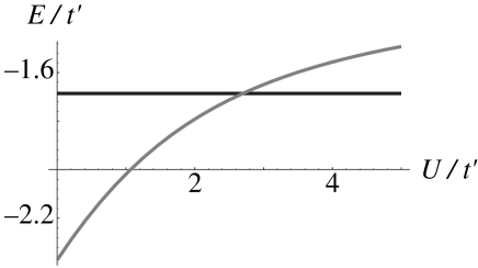
Figure 7: The $U$ dependence of $E_{\rm min}(0)$ (gray curve) and $E_{\rm min}(1)$ (black line) in the toy model with $t=t^{\prime}/2$. We have ferromagnetism in the sense that $E_{\rm min}(0)>E_{\rm min}(1)$ when $U$ is sufficiently large. We find that ferromagnetism is a “nonperturbative” phenomenon.

Let us briefly look at the cases with finite $U$. In Figure 7, we plotted $E_{\rm min}(0)$ and $E_{\rm min}(1)$ for the toy model with $t=t^{\prime}/2$ as functions of $U$. (See Definition 2.1.) As is suggested by the result in the $U\to\infty$ limit, we have ferromagnetism in the sense that $E_{\rm min}(0)>E_{\rm min}(1)$ when $U$ is sufficiently large. A level crossing takes place at finite $U$, and the system is no longer ferromagnetic for small $U$. Even in the simplest toy model, ferromagnetism is a “nonperturbative” phenomenon which takes place only when $U$ is sufficiently large.

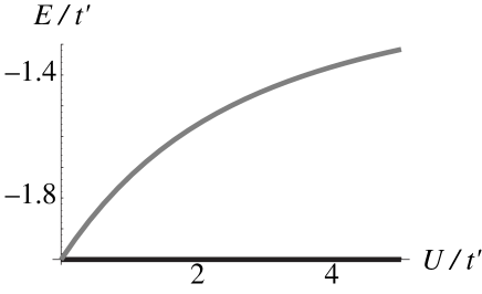
Figure 8: The $U$ dependence of $E_{\rm min}(0)$ (gray curve) and $E_{\rm min}(1)$ (black line) in the toy model with $t=t^{\prime}$. Only for this special parameter, we have ferromagnetism $E_{\rm min}(0)>E_{\rm min}(1)$ for any value of $U>0$. One can regard this case as the simplest example of the flat-band ferromagnetism that we will discuss in Section 6.4.

The only exception is the case with $t=t^{\prime}$. See Figure 8. For this parameter value, the ground states are degenerate in spin when $U=0$. Ferromagnetic state is the only ground state for $U>0$.

From Figures 7 and 8, we find that the energy $E_{\rm min}(1)$ of ferromagnetic states is independent of $U$. As we see in the following, this is a general property of ferromagnetic eigenstates in the Hubbard model. An arbitrary state $\Psi$ which has total spin $S_{\rm tot}=S_{\rm max}$ can be written as a superposition of states which are obtained by rotating the state $\widetilde{\Psi}$ which consists only of $\uparrow$ spin electrons. If one operates the interaction Hamiltonian $H_{\rm int}$ (2.5) onto the state $\widetilde{\Psi}$, one has $H_{\rm int}\widetilde{\Psi}=0$ because $n_{x,\downarrow}\widetilde{\Psi}=0$. Since the interaction Hamiltonian (2.5) is invariant under rotation in spin space, we have shown that $H_{\rm int}\Psi=0$. One might say that states with saturated magnetization do not feel Hubbard type interaction at all. This is one of convenient (but “oversimplified”) features in discussing saturated ferromagnetism in the Hubbard model.

6.3 Nagaoka’s Ferromagnetism

The transitions between the states in Figure 6 are generated by hoppings of electrons. One can also regard that the transitions are caused by hoppings of a single hole, which is the site without electrons. At least in the limit $U\to\infty$, one can say that the origin of ferromagnetism in the toy model is the motion of a single hole, which mix up various spin configurations with proper signs.

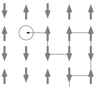
Figure 9: Schematic picture about the origin of Nagaoka’s ferromagnetism. When the hole hops around the lattice, the spin configuration is changed. For a model with $t_{x,y}\geq 0$, the hole motion produces a precise linear combination of various spin configurations which leads to ferromagnetic state.

As Nagaoka [25] demonstrated rigorously, there is a class of many electron models in which saturated ferromagnetism is generated by exactly the same mechanism. See Figure 9. Nagaoka’s theorem (in the extended form of [26] whose complete proof can be found in [2]) is as follows.

Theorem 6.3 (Nagaoka’s ferromagnetism)

Take an arbitrary finite lattice $\Lambda$, and assume that $t_{x,y}\geq 0$ for any $x\neq y$, and $U_{x}=\infty$ for any $x\in\Lambda$. We fix the electron number as $N_{\rm e}=|\Lambda|-1$. Then among the ground states of the model, there exist states with total spin $S_{\rm tot}=S_{\rm max}(=N_{\rm e}/2)$. If the system further satisfies the connectivity condition, then the ground states have $S_{\rm tot}=S_{\rm max}(=N_{\rm e}/2)$ and are nondegenerate apart from the trivial spin degeneracy.

The connectivity condition is a simple condition which holds on most of the lattices in two or higher dimensions, including the square lattice, the triangular lattice, or the cubic lattice. To be precise the condition requires that “by starting from any electron configuration on the lattice and by moving around the hole along nonvanishing $t_{x,y}$, one can get any other electron configuration.”

Thouless also reached a similar conclusion [27], but Nagaoka’s treatment covers a larger class of models including non-bipartite systems. The proof of Nagaoka’s theorem (especially the recent proof in [26]) is surprisingly simple. It essentially uses the Perron-Frobenius argument exactly the same as that we used in Section 6.2 to determine the total spin of the ground state of the toy model.

The requirements that $U$ should be infinitely large and there should be exactly one hole are indeed rather pathological. Nevertheless, the theorem is very important since it showed for the first time in a rigorous manner that quantum mechanical motion of electrons and strong Coulomb repulsion can generate ferromagnetism. The conclusion that the system which has one less electron than the half-filled model exhibits ferromagnetism is indeed surprising. This is a very nice example which demonstrates that strongly interacting electron systems produce very rich physics.

It is desirable to extend Nagaoka’s ferromagnetism to systems with a finite $U$ and with a finite density of holes. Although more than thirty years have passed since Nagaoka’s and Thouless’s papers, it is still not known if such extensions are possible. There are, however, considerable amount of rigorous works which establish that saturated ferromagnetism does not take place in certain situations. See, for example, [28, 29, 30, 31, 32, 33].

6.4 Mielke’s Ferromagnetism and Flat-Band Ferromagnetism

Let us once again look at the toy model of section 6.2. As is shown in Figure 8, the ground state of the model exhibits ferromagnetism for any $U>0$ for the special choice of the parameters $t=t^{\prime}>0$. For this choice of parameters, the energy eigenvalues of the corresponding Schrödinger equation are $\varepsilon_{1}=\varepsilon_{2}=-t^{\prime}$, and $\varepsilon_{3}=2t^{\prime}$. The single-electron ground states are doubly degenerate. As a consequence, the ground states of the two electron system with $U=0$ are also degenerate, and can have $S_{\rm tot}=0$ or $S_{\rm tot}=1$. The degeneracy is lifted for $U>0$, and the ferromagnetic state is “selected” as the true and unique ground state. It is crucial here that the dimension of the degeneracy in the single-electron ground states (which is two) is the same as the electron number $N_{\rm e}=2$.

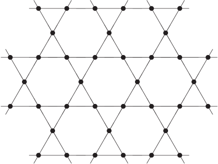
Figure 10: The Hubbard model on the kagomé lattice is a typical example which exhibits flat-band ferromagnetism. “Kagomé” is a Japanese word for a pattern of woven bamboo of baskets.

Mielke [34] showed that there is a class of Hubbard models with many electrons which show saturated ferromagnetism through a somewhat similar mechanism. Take, for example, the kagomé lattice of Figure 10, and define a Hubbard model on it by setting $t_{x,y}=t>0$ for neighboring sites $x,y$, $t_{x,y}=0$ for other situations, and $U_{x}=U\geq 0$ for any $x\in\Lambda$. It is worth mentioning that the kagomé lattice of Figure 10 can be regarded as constructed by putting together many copies of the lattice used in the toy model (Figure 5). The energy eigenvalues of the corresponding Schrödinger equation can be shown to satisfy $\varepsilon_{1}=\varepsilon_{2}=\cdots=\varepsilon_{M}=-2t$, and $\varepsilon_{j}>-2t$ for $j>M$. Here the dimension $M$ of the degeneracy of the single-electron ground states is given by $M=(|\Lambda|/3)+1$, and is proportional to the lattice size.

We shall fix the electron number as $N_{\rm e}=M$, the same as the dimension of the degeneracy.

Let us consider the case with $U=0$ first. Let $A$ and $B$ be arbitrary subsets of $\left\{1,2,\ldots,N_{\rm e}\right\}$ which satisfy $|A|+|B|=N_{\rm e}$, and consider the state $\Phi_{A,B}$ (3.4) obtained by creating the corresponding single-electron eigenstates. In the present model on the kagomé lattice, the fermion operator $a^{\dagger}_{j,\sigma}$ (3.2) creates one of the single-electron ground states with the energy $\varepsilon=-2t$. This means that we have $H_{\rm hop}\Phi_{A,B}=-2tN_{\rm e}\Phi_{A,B}$ for arbitrary choice of $A$ and $B$, and hence $\Phi_{A,B}$ is a ground state of $H=H_{\rm hop}$. We find that the ground states are highly degenerate, and can have $S_{\rm tot}=0,1,\ldots,S_{\rm max}=M/2$ (or $S_{\rm tot}=1/2,\ldots,S_{\rm max}$).

What is the effect of nonvanishing Coulomb interaction $U$ in such a situation? Let us denote by $\Phi_{\uparrow}$ the state obtained by setting $A=\left\{1,2,\ldots,N_{\rm e}\right\}$ and $B=\emptyset$ in $\Phi_{A,B}$. Of course $\Phi_{\uparrow}$ is one of the ground states of $H_{\rm hop}$. As we discussed at the end of Section 6.2, the state $\Phi_{\uparrow}$ which consists only of $\uparrow$ spin electrons “does not feel” Hubbard type Coulomb interaction. This means that we have $H_{\rm int}\Phi_{\uparrow}=0$. Since $0$ is the minimum possible eigenvalue of $H_{\rm int}$, we find that the state $\Phi_{\uparrow}$ is a ground state of the total Hamiltonian$H=H_{\rm hop}+H_{\rm int}$ for any $U>0$.

These are all simple observations. A really interesting problem is whether there can be ground states other than $\Phi_{\uparrow}$ when $U>0$. The following theorem due to Mielke shows that the ferromagnetic state is indeed “selected” as the true ground state exactly as in the toy model.

Theorem 6.4 (Mielke’s flat-band ferromagnetism)

Consider the Hubbard model on the kagomé lattice described above. For any $U>0$, the ground states have $S_{\rm tot}=S_{\rm max}(=M/2)$ and are nondegenerate apart from the trivial spin degeneracy.

Mielke [35] also extended his results to the situation where the electron density $N_{\rm e}/|\Lambda|$ is less than $1/3$ but close to $1/3$.

In Mielke’s work, it was proved for the first time that the Hubbard model with finite $U$ can exhibit saturated ferromagnetism. The model is very simple, and the result is very important. As far as the author knows, there had been no discussions about the possibility of ferromagnetism in the Hubbard model on the kagomé lattice. Mielke’s work is not only mathematically rigorous, but important from physicists’ point of view as it opened a new way of approaching itinerant electron ferromagnetism.

Mielke’s proof of his main theorem is an elegant induction which makes use of a graph theoretic language. The proof is not at all trivial since the problem is intrinsically a many-body one. However, there is a very special feature of the model that any ground state of the total Hamiltonian $H=H_{\rm hop}+H_{\rm int}$ is at the same time a ground state of each of $H_{\rm hop}$ and $H_{\rm int}$. Because of this property, one does not have to face the very difficult problem in many-body problems called the “competition between $H_{\rm hop}$ and $H_{\rm int}$.” That one has ferromagnetism in this model for any $U(>0)$ is closely related to this fact.

Mielke’s theorem applies not only to the Hubbard model on the kagomé lattice but to those on a wide class of lattices called line graphs. In all of these models, the ground states in the corresponding single-electron Schrödinger equation are highly degenerate. There have been constructed [36, 37] other examples of Hubbard models in which the corresponding single-electron ground states are highly degenerate, and exhibit saturated ferromagnetism for any $U>0$. Ferromagnetism in the examples of Mielke and in [36, 37] are now called flat-band ferromagnetism. Mielke [38] obtained a necessary and sufficient condition for a Hubbard model with highly degenerate single-electron ground states to exhibit saturated ferromagnetism. It is interesting that Lieb’s ferrimagnetism discussed in Section 5.3 resembles flat-band ferromagnetism in that the corresponding single-electron spectrum has a bulk degeneracy.

It is needless to say that the models in which single-electron ground states are highly degenerate are rather singular. By adding a generic small perturbation to the hopping Hamiltonian, the degeneracy is lifted in general, and one gets a nearly flat lowest band rather than a completely flat one. A very interesting and important problem is whether ferromagnetism remains stable after such a perturbation is added. Of course one does not have ferromagnetism for small enough $U$ if the bulk degeneracy in the single-electron ground states is lifted. What one expects is that ferromagnetism remains stable when $U$ is sufficiently large. (Recall that in the toy model of Section 6.2, we had ferromagnetism for all $U>0$ only for the special choice of parameters $t=t^{\prime}$.) There are some indications (from numerical or variational calculations) that ferromagnetism is stable under perturbation. As for rigorous results, stability of ferromagnetism under single-spin flip is proved in [39, 40] for the model obtained by adding arbitrary small perturbation to the Hubbard model of [36, 37]. As for a special class of perturbations, the problem of stability of ferromagnetism is completely solved as we shall see in the next section.

6.5 Ferromagnetism in a Non-Singular Hubbard model

We have seen two theorems which show that certain Hubbard models exhibit saturated ferromagnetism. In Nagaoka’s theorem, it is assumed that the system has exactly one hole, and has infinitely large Coulomb interaction. In Mielke’s theorem and other flat-band ferromagnetism, it is essential that the single-electron ground states have a bulk degeneracy. Is it possible to prove the existence of saturated ferromagnetism in a non-singular Hubbard model which have finite $U$ and in which the single-electron spectrum is not singular? Recently such examples were constructed [41].

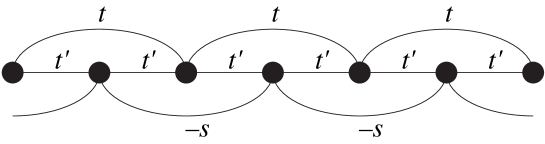
Figure 11: An example of non-singular Hubbard model which exhibits saturated ferromagnetism [41]. If we look at three adjacent sites, the lattice structure and the hopping resemble that of the toy model of Figure 5.

For simplicity, we concentrate on the simplest models in one dimension. Take the one dimensional lattice $\Lambda=\left\{1,2,\ldots,N\right\}$ with $N$ sites (where $N$ is an even integer), and impose a periodic boundary condition by identifying the site $N+1$ with the site $1$. The hopping matrix is defined by setting $t_{x,x+1}=t_{x+1,x}=t^{\prime}$ for any $x\in\Lambda$, $t_{x,x+2}=t_{x+2,x}=t$ for even $x$, $t_{x,x+2}=t_{x+2,x}=-s$ for odd $x$, and $t_{x,y}=0$ otherwise. Here $t>0$ and $s>0$ are independent parameters, but the parameter $t^{\prime}$ is determined as $t^{\prime}=\sqrt{2}(t+s)$. As can be seen from Figure 11, the model has two kinds of next nearest neighbor hoppings $t$ and $-s$, as well as the nearest neighbor hopping $t^{\prime}$. If we look at an odd site and the two neighboring even sites, the model is exactly the same as the toy model we treated in Section 6.2. Roughly speaking, this resemblance is the basic origin of ferromagnetism in the present model. We also note that because there are next nearest neighbor hoppings, Lieb-Mattis theorem (Theorem 4.1) does not apply to the present model.

The single electron energy eigenvalue in this model can be expressed by using the wave number $k=2\pi n/N$ ($n=0,\pm 1,\ldots,\pm\left\{(N/4)-1\right\},N/4$) as $\varepsilon_{1}(k)=-2t-2s(1+\cos 2k)$ and $\varepsilon_{2}(k)=2s+2t(1+\cos 2k)$. There are two bands, and each of them has healthy dispersion.

As for the Coulomb interaction, we set $U_{x}=U>0$ for any $x\in\Lambda$. We fix the electron number as $N_{\rm e}=N/2$. In terms of filling factor, this corresponds to the quarter filling. The maximum possible value of total spin is $S_{\rm max}=N/4$.

Unlike in flat-band ferromagnetism, there is no saturated ferromagnetism when $U$ is sufficiently small. Theorem 6.1 ensures that the ground state have $S_{\rm tot}<S_{\rm max}$ if $U<4s$. If the present system were to show saturated ferromagnetism, it should be in the “nonperturbative” region with sufficiently large $U$. The following theorem of [41] provides such a nonperturbative result.

Theorem 6.5 (Ferromagnetism in a non-singular Hubbard model)

Suppose that the two dimensionless parameters $t/s$ and $U/s$ are sufficiently large. Then the ground states have $S_{\rm tot}=S_{\rm max}(=N/4)$ and are nondegenerate apart from the trivial spin degeneracy.

The theorem is valid, for example, when $t/s\geq 4.5$ if $U/s=50$, and $t/s\geq 2.6$ if $U/s=100$. The ferromagnetic ground state can be constructed in exactly the same manner as $\Phi_{\uparrow}$ in the previous section.

Although the model is rather artificial, this is the first rigorous example of saturated ferromagnetism in a non-singular Hubbard model on which we have to overcome the competition between $H_{\rm int}$ and $H_{\rm hop}$. In a class of similar models, it is also proved that low-lying excitation above the ground state has a normal dispersion relation of a spin-wave excitation [41, 40]. Starting from a Hubbard model model of itinerant electrons, the existence of a “healthy” ferromagnetism is established rigorously.

If we set $s=0$ in the present model, the ground states of the single-electron Schrödinger equation become $N/2$-fold degenerate. In this case, the model exhibits saturated ferromagnetism (flat-band ferromagnetism) for any $U>0$. Theorem 6.5 for $s\neq 0$ can be regarded as a solution to the problem about stability of flat-band ferromagnetism against perturbation to the hopping Hamiltonian.

The basic strategy in the proof of Theorem 6.5 is first to establish the existence of saturated ferromagnetism in a Hubbard model on a chain with five sites, and then “connect” together these local ferromagnetism to get ferromagnetism in the whole system. Generally speaking, this is a crazy idea. In a quantum mechanical system, especially in a system with healthy dispersion (like the present one), electrons have strong tendency to extend in a large region and reduce kinetic energy. To confine electrons in a finite region usually costs extra energy. To obtain exact information about large system from smaller system seems to be impossible. The reasons that such a strategy works in the present model are twofold. One is the special construction of the model. The other is that we described electron states using a language which takes into account both the particle-like character of electrons and the band structure of the model. The latter is a natural strategy to deal with the Hubbard model in which wave-particle dualism generate interesting physics.

It is believed that the ground states of the present Hubbard model describes an insulator. When the electron number is less than $N/2$, we expect that the present model exhibits metallic ferromagnetism in which the same set of electrons participate in conduction as well as magnetism. For the moment, we still do not know of any useful ideas in proving this fascinating conjecture.

I wish to thank Kenn Kubo and Balint Tóth for useful comments on the early version of the present article.

References

- [1] E. H. Lieb, in Proceedings of 1993 conference in honor of G.F. Dell’Antonio, Advances in Dynamical Systems and Quantum Physics, pp. 173-193, World Scientific (1995), Proccedings of 1993 NATO ASW The Physics and Mathematical Physics of the Hubbard Model, Plenum (in press), and Proceedings of the XIth International Congress of Mathematical Physics, Paris, 1994, D. Iagolnitzer ed., pp. 392-412, International Press (1995). Archived as cond-mat/9311033.
- [2] H. Tasaki, “From Nagaoka’s ferromagnetism to flat-band ferromagnetism and beyond: An introduction to ferromagnetism in the Hubbard model”, preprint (1997), cond-mat/9712219.
- [3] R. Strack and D. Vollhardt, J. Low Temp. Phys. 99, 385 (1995).
- [4] J. de Boer, V. E. Korepin and A. Schadschneider, Phys. Rev. Lett. 74, 789 (1995).
- [5] J. de Boer and A. Schadschneider. Phy. Rev. Lett. 75, 4298 (1995).
- [6] D. Vollhardt, N. Blümer, K. Held, M. Kollar, J. Schlipf, and M. Ulmke, Z. Phys. B 103, 283 (1997).
- [7] E. H. Lieb and D. Mattis, Phy. Rev. 125, 164 (1962).
- [8] E. H. Lieb and D. Mattis, J. Math. Phys. 3, 749 (1962).
- [9] D. Ghosh, Phy. Rev. Lett. 27, 1584 (1971).
- [10] T. Koma and H. Tasaki, Phy. Rev. Lett. 68, 3248 (1992).
- [11] M. Yamanaka, M. Oshikawa, and I. Affleck, Phys. Rev. lett. 79, 1110, (1997).
- [12] M. Oshikawa and M. Yamanaka, in preparation.
- [13] E. H. Lieb, Phy. Rev. Lett. 62, 1201 (1989), errata Phy. Rev. Lett. 62, 1927 (1989)
- [14] T. Koma and H. Tasaki, J. Stat. Phys. 76, 745 (1994).
- [15] S. Q. Shen, Z. M. Qiu, and G. S. Tian, Phy. Rev. Lett. 72, 1280 (1994).
- [16] S. Q. Shen, Phys. Rev. B 53, 14252 (1996).
- [17] F. Dyson, E. H. Lieb, and B. Simon, J. Stat. Phys. 18, 335 (1978).
- [18] T. Kennedy, E. H. Lieb, and B. S. Shastry, J. Stat. Phys. 53, 1019 (1988).
- [19] E. H. Lieb, M. Loss, and R. McCann, J. Math. Phys. 34, 891 (1993).
- [20] E. H. Lieb, Phy. Rev. Lett. 73, 2158 (1994).
- [21] N. Macris and B. Nachtergaele, J. Stat. Phys. 85, 754 (1996)
- [22] B. Nachtergaele and E. H. Lieb, Phys. Rev. B51, 4777 (1995).
- [23] K. Kubo and K. Kishi, Phys. Rev. B41, 4866 (1990).
- [24] P. Pieri, S. Daul, D. Baeriswyl, M. Dzierzawa, and P. Fazekas, Phys. Rev. B45, 9250 (1996).
- [25] Y. Nagaoka, Phy. Rev. 147, 392 (1966).
- [26] H. Tasaki, Phy. Rev. B40, 9192 (1989).
- [27] D. J. Thouless, Proc. Phys. Soc. London 86, 893 (1965).
- [28] B. Douçot and X. G. Wen, Phy. Rev. B40, 2719 (1989).
- [29] B. S. Shastry, H. R. Krishnamurthy, and P. W. Anderson, Phy. Rev. B41, 2375 (1990).
- [30] B. Tóth, Lett. Math. Phys. 22, 321 (1991).
- [31] A. Sütő, Commun. Math Phys. 40, 43 (1991).
- [32] T. Hanisch and E. Müller-Hartmann, Ann. Physik 2, 381 (1993).
- [33] T. Hanisch, G. S. Uhrig, and E. Mueller-Hartmann, preprint (1997), cond-mat/9707286.
- [34] A. Mielke, J. Phys. A24, 3311 (1991).
- [35] A. Mielke, J. Phys. A25, 4335 (1992).
- [36] H. Tasaki, Phy. Rev. Lett. 69, 1608 (1992).
- [37] A. Mielke and H. Tasaki, Commun. Math Phys. 158, 341 (1993).
- [38] A. Mielke, Phys. Lett. A174, 443 (1993).
- [39] H. Tasaki, Phy. Rev. Lett. 73, 1158 (1994).
- [40] H. Tasaki, J. Stat. Phys. 84, 535 (1996).
- [41] H. Tasaki, Phy. Rev. Lett., 75, 4678 (1995).
- [42] H. Tasaki, “Ferromagnetism in the Hubbard model: A constructive approach”, in preparation.
- [43] U. Brandt and A. Giesekus. Phy. Rev. Lett. 68, 2648 (1992).
- [44] A. Mielke, J. Phys. A25, 6507 (1992)
- [45] R. Strack, Phys. Rev. Lett. 70, 833 (1993).
- [46] H. Tasaki, Phys. Rev. Lett. 70, 3303 (1993).
- [47] H. Tasaki, Phys. Rev. B49, 7763 (1993).
- [48] P.-A. Bares and P. A. Lee, Phys. Rev. B49, 8882 (1993).
- [49] M. Yamanaka, S. Honjou, Y. Hatsugai and M. Kohmoto, J. Stat. Phys. 84, 1133 (1996).