In presenting this thesis in partial fulfilment of the requirements for an advanced degree at the University of British Columbia, I agree that the Library shall make it freely available for reference and study. I further agree that permission for extensive copying of this thesis for scholarly purposes may be granted by the head of my department or by his or her representatives. It is understood that copying or publication of this thesis for financial gain shall not be allowed without my written permission.

  

Department of Physics

The University of British Columbia

2075 Wesbrook Place

Vancouver, Canada

V6T 1W5

Date:

  

Abstract

A comprehensive theory of nuclear magnetic relaxation in $S=1$ Haldane gap materials is developed using nonlinear-$\sigma$, boson and fermion models. We find that at temperatures much smaller than the lowest gap the dominant contribution to the relaxation rate comes from two magnon processes with $T_{1}^{-1}\sim e^{-\Delta_{m}/T}$, where $\Delta_{m}$ is the smallest gap corresponding to a polarization direction perpendicular to the field direction. As the gap closes, we find that the dominant contribution comes from one magnon processes, and the result depends on the symmetry of the Hamiltonian. Overall the models agree qualitatively, except near the critical regime, where the fermion model is shown to be the best description. We include a thorough discussion of the effects of interchain couplings, nearest neighbour hyperfine interactions and crystal structure, and introduce a new theory of impurities corresponding to broken chain ends weakly coupled to bulk magnons. The work is then applied to recent measurements on NENP. We find overall fair agreement between available $T^{-1}_{1}$ data and our calculations. We finish by suggesting further experimental tests of our conclusions.

Table of Contents

toc

List of Figures

lof

Chapter 1 Introduction and Background

1.1 Introduction

In 1983, Haldane derived his famous result stating that integer spin one dimensional Heisenberg antiferromagnets featured a gap in their low energy excitation spectrum [1]. Since then, much effort has been devoted to further exploration of such systems, both experimentally and theoretically. The purpose of this work is to develop a theoretical framework for the understanding of low energy experiments on one dimensional Haldane gap materials. In particular, we focus on the nuclear magnetic relaxation rate, $T_{1}^{-1}$, although the work has relevance to many other techniques. By studying this thesis, it is hoped that the reader can become familiar with the tools used to understand integer spin Heisenberg antiferromagnetic chains with anisotropies, and can apply these tools to the analysis of real systems.

There are, essentially, three important models that have so far been used to describe the system. In the later sections of this chapter we review the competing descriptions of $S=1$ antiferromagnetic spin-chains, paying some attention to their advantages and shortcomings. We start by outlining the traditional spin-wave theory used to model antiferromagnetism in higher dimensions. After illustrating the deficiencies in this approach, we describe the Nonlinear $\sigma$ (NL$\sigma$) model in some detail. This is followed by an analysis of a simplified yet closely related Landau-Ginsburg boson model. Last, we discuss a free fermion model used recently to successfully treat the case of anisotropic spin-chains. We end the chapter with background on the nuclear magnetic relaxation rate, $1/T_{1}$, for nuclear spins coupled to the spin-chain through hyperfine interactions.

Chapter Two focuses on the details of the models, building the tools necessary for a detailed analysis. We discuss the temperature and magnetic field dependence of the NL$\sigma$ model and its possible relevance to the spectrum of the boson model, as well as cite some exact results available in cases of high symmetry. We also diagonalize the free boson and fermion field theories, including on-site anisotropy effects. We derive matrix elements of the uniform spin operator between one particle states of magnetic excitations. These are used to compare the different models.

Chapter Three explicitly describes the calculation of NMR $T_{1}^{-1}$, considering various symmetries of the Hamiltonian. We identify the leading mechanisms for low temperature relaxation in the presence of a magnetic field. We discuss three regimes corresponding to different magnitudes of the applied external magnetic field, giving expressions for the rate in each case. We discover that at temperatures much lower than the smallest gap the uniform part of the spin operator contributes most to the relaxation rate; in the absence of interactions, this corresponds to two magnon processes. The rate is found to be $T_{1}^{-1}\sim e^{-\Delta_{m}/T}$, where $\Delta_{m}$ is the smallest gap corresponding to a polarization direction perpendicular to the magnetic field. As the externally applied magnetic field approaches a critical value, one of the gaps closes and we find the dominant process to be one magnon, corresponding to contributions from the staggered part of the spin. In this regime, we show that the fermion model is the best description and that the expression for $T_{1}^{-1}$ depends on the symmetry of the Hamiltonian.

Chapter Four deals with intrinsic effects which must be taken into account when analyzing experimental data. We discuss nearest neighbour hyperfine interactions; we show that these will contribute to order $A_{nn}/A$, the ratio of the nearest neighbour coupling to the local coupling. We also consider interchain couplings and show that they introduce a natural infrared cutoff to the diverging density of states at the gap; for sufficiently long chains, they also densely fill the energy intervals between states along a finite chain. Finally, we introduce a new impurity theory to explain the effects of nearly free spin-$\frac{1}{2}$ chain end degrees of freedom. We find that the states formed by such end spins in the gap, can give rise to non-trivial relaxation when coupled to the bulk excitations.

Chapter Five applies the theory to recent experiments on the well studied material, $Ni(C_{2}H_{8}N_{2})_{2}NO_{2}(ClO_{4})$ (NENP). We take a close look at the crystal structure of NENP and identify possible terms which may be present in the Hamiltonian. We also note the fact, hitherto neglected, that NENP possesses two inequivalent chains in each unit cell. The results of Chapters Three and Four are then used to analyze experimental data. We find reasonable agreement for a magnetic field placed along the crystal $c$-axis of NENP, and an unexpected discrepancy for a magnetic field placed along the chain axis. The impurity theory is used to model low field data with qustionable results.

The final chapter proposes further experimental tests of the theoretical predictions of this work. We suggest elastic neutron, electron spin resonance and further NMR studies to verify our own.

1.2 Spin-wave Theory

The Heisenberg Hamiltonian describing the isotropic antiferromagnetic spin-chain is

$$H=J\sum_{i}\mbox{ {\boldmath$\vec{S}$}}_{i}\cdot\mbox{ {\boldmath$\vec{S}$}}_{i+1}\mbox{\hskip 36.135pt}J>0$$ (1.1)

This arises naturally from the Hubbard model for insulators at ‘half’ filling [3]. To understand where this might come from, we follow the case where there is a triplet of possible spin states per site. On each site there are a number of valence electrons (eight valence electrons in the $d$ shell of $Ni^{+2}$, for example); the degenerate electronic levels are split in a way determined by Hund’s rules and the symmetry of the crystal fields surrounding the ion. In some special cases (as with $Ni^{+2}$ in a field with octahedral symmetry), a degenerate triplet of states lies lowest. The ensuing low energy physics can be essentially described using effective spin 1 operators [4]. By ‘half’ filling, we mean that there is an effective $S=1$ triplet of states for every site in the chain (ie. there are two singly occupied orbitals on each site. Other orbitals are either empty or doubly occupied. Spins in singly occupied orbitals are aligned by Hund’s rules.) Antiferromagnetism comes from allowing a small amplitude for nearest neighbour hopping which is highly suppressed by coulomb repulsion from the electrons already occupying the site.

In the quantum case, the spin operators have the commutation relations:

$$[S^{a}_{i},S^{b}_{j}]=i\delta_{ij}\sum_{c}\epsilon^{abc}S^{c}_{i},\mbox{\hskip 14.45377pt}\mbox{ {\boldmath$\vec{S}$}}_{i}\cdot\mbox{ {\boldmath$\vec{S}$}}_{i}=s(s+1)$$ (1.2)

where $\delta_{ij}$ is the Kronecker Delta Function and $\epsilon^{abc}$ is the completely antisymmetric Levi-Civita symbol.

It is easy to see that the classical Néel ground state with alternating spins is not the quantum ground state. To this end we write the Hamiltonian in terms of raising and lowering spin operators:

$$S^{\pm}\equiv S^{x}\pm iS^{y}$$

$$H=J\sum_{i}\left[S_{i}^{z}S_{i+1}^{z}+\frac{1}{2}(S^{+}_{i}S^{-}_{i+1}+S^{-}_{i}S^{+}_{i+1})\right]$$ (1.3)

The Néel ground state is composed of spins alternating in quantum numbers $s^{z}$ between sites.

$$|\mbox{N\'{e}el}>=|s^{z}_{1}=+1,s^{z}_{2}=-1,s^{z}_{3}=+1,...,s^{z}_{N}=-1>$$ (1.4)

This state is clearly not an eigenstate of the above Hamiltonian since upon acting on it, the $S^{+}_{i}S^{-}_{i+1}$ terms in the Hamiltonian generate states with $m_{i}=0$. To proceed in understanding the low energy properties one usually assumes that the ground state is approximately Néel with quantum fluctuations. The picture is that of zero point motion about the positions of the classical Néel spins. What we will shortly see is that the assumption of small fluctuations breaks down in one dimension.

The conventional approach makes use of the Holstein-Primakov transformation. One begins by dividing the chain into two sublattices, “A” and “B”, with adjacent sites on separate sublattices. On sublattice “A” one defines

$$S^{z}_{i}=s-a^{\dagger}_{i}a_{i},\mbox{\hskip 14.45377pt}S^{-}_{i}=a^{\dagger}_{i}\sqrt{2s-a^{\dagger}_{i}a_{i}}$$ (1.5)

On sublattice “B” we have

$$S^{z}_{i+1}=-s+b^{\dagger}_{i}b_{i},\mbox{\hskip 14.45377pt}S^{+}_{i+1}=b^{\dagger}_{i}\sqrt{2s-b^{\dagger}_{i}b_{i}}$$ (1.6)

$a$ and $b$ are usual bosonic operators with commutation relations:

$$[a,a^{\dagger}]=[b,b^{\dagger}]=1,\mbox{\hskip 14.45377pt}[a,a]=[b,b]=0$$ (1.7)

It can be checked that (1.5) and (1.6) preserve the correct spin commutation relations and the constraint $\mbox{ {\boldmath$\vec{S}$}}_{i}\cdot\mbox{ {\boldmath$\vec{S}$}}_{i}=s(s+1)$. The Néel ground state is one without bosons. So far no approximations have entered into the picture. However, to make progress, we assume that $s$ is large. This is equivalent to a semi-classical approximation since for $s\rightarrow\infty$ the commutator of the spins will have much smaller eigenvalues than the square of the spin variables

$$[S^{a},S^{b}]=i\sum_{c}\epsilon^{abc}S^{c}=O(s)\ll O(s^{2})$$ (1.8)

We expand the spin operators to give

$$S^{-}_{i}=a^{\dagger}_{i}\sqrt{2s},\mbox{\hskip 14.45377pt}S^{+}_{i+1}=b^{\dagger}_{i}\sqrt{2s}$$ (1.9)

To leading order, the Hamiltonian reduces to

$$H=J\sum_{i}\left[-s^{2}+s(2a^{\dagger}_{i}a_{i}+2b^{\dagger}_{i}b_{i}+a_{i}b_{i}+b_{i-1}a_{i}+b^{\dagger}_{i}a^{\dagger}_{i}+a^{\dagger}_{i}b^{\dagger}_{i-1})+O(1)\right]$$ (1.10)

Fourier transforming:

$$a_{j}=\frac{1}{\sqrt{N}}\sum_{n=-\frac{N}{2}}^{\frac{N}{2}}e^{i2\pi jn/N}a_{k}$$ (1.11)

with a similar expression for $b$; $N$ is the number of sites on each sublattice. Ignoring the constant term, we rewrite (1.10) as

$$H=2Js\sum_{k}\left[a^{\dagger}_{k}a_{k}+b^{\dagger}_{k}b_{k}+(1+e^{2ika})(a_{k}b_{-k}+b_{k}^{\dagger}a^{\dagger}_{-k})\right]$$ (1.12)

$2a$ is the sublattice spacing and $k=\pi n/Na$ for $n\in[-\frac{N}{2},\frac{N}{2}]$. We now make the Bogoliubov transformation,

$$c_{k}=u_{k}a_{k}-v_{k}b_{-k}^{\dagger}$$

$$d_{k}=u_{k}b_{-k}-v_{k}a^{\dagger}_{k}$$ (1.13)

where,

$$u_{k}=\frac{ie^{ika/2}}{\sqrt{2}}\left(1+\csc(ka)\right)^{1/2}$$

$$v_{k}=\frac{-ie^{-ika/2}}{\sqrt{2}}\left(-1+\csc(ka)\right)^{1/2}$$ (1.14)

The $d$’s and $c$’s are spin wave operators corresponding to magnetic excitations (magnons) with $S^{z}=\pm 1$ respectively. This transformation preserves the commutation relations and the Hamiltonian can now be written as

$$H=2Js\sum_{k}\sin(|ka|)\left(c^{\dagger}_{k}c_{k}+d^{\dagger}_{k}d_{k}\right)$$ (1.15)

We see that this low energy description implies the spins are in some coherent state of $a$’s and $b$’s built on the Néel state, but there are long wavelength Goldstone modes with dispersion relation $\omega=2Js|ka|$ which allow each of the sublattice magnetization vectors to make long wavelength rotations. To ensure consistency, we now look at the expectation value of the magnetization (say, on the “A” sublattice), hoping to see that we get the semi-classical result $<S^{z}_{i}>=s-O(1)$. We invert the Bogoliubov transformation to get

$$a_{k}=u_{k}^{\ast}c_{k}+v_{k}d^{\dagger}_{k}$$ (1.16)

and compute

$$<S^{z}_{i}>=s-<a^{\dagger}_{i}a_{i}>=s-\frac{1}{N}\sum_{k}<a^{\dagger}_{k}a_{k}>$$

$$=s-a\int\frac{dk}{2\pi}|v_{k}|^{2}=s-a\int\frac{dk}{4\pi}\left(\csc(ka)-1\right)$$ (1.17)

The last line follows from (1.16) and the fact that the true ground state has zero spin wave occupation number. The problem is now apparent: low wavelength modes cause $<s-S^{z}>$ to diverge logarithmically. The semi classical picture of a Néel-like ground state is completely off. This is special to 1 dimension and actually arises as a general consequence of Coleman’s theorem [5]; it states that in $(1+1)$ dimensions, infrared divergences associated with Goldstone bosons will always wash out the classical value of the order parameter rendering spontaneous symmetry breaking of continuous symmetries impossible. One is therefore forced to look elsewhere in order to describe the low energy physics of the Heisenberg model.

1.3 Non-Linear $\sigma$ (NL$\sigma$) Model

The most consistent continuum model derivable from Eqn. (1.1) is the Nonlinear $\sigma$ model. In addition to being a continuum model (valid only in the long wave length limit), it is also based on a large $s$ approximation. One introduces two fields: $\vec{\phi}$ — corresponding to the Néel order parameter, and $\bf{\vec{l}}$ — the uniform magnetization. The spin variable, $\bf{\vec{S}}$ is defined in terms of these fields via

$${\bf\vec{S}}(x)=(-1)^{x}s\mbox{\boldmath$\vec{\phi}$}(x)+{\bf\vec{l}}(x)$$ (1.18)

The conventional derivation defines these variables on the lattice and a continuum limit is taken in the semi-classical large $s$ approximation to arrive at the NL$\sigma$ model Hamiltonian [6]. There are several problems with this approach. First, parity is broken in intermediate steps and is eventually restored in the continuum limit. Second, and more importantly, the crucial topological term which is found in the continuum Hamiltonian is derived without clear notions of how $1/s$ corrections may be made. A much more elegant approach will be reviewed here. We will make use of path integral formalism based on independent derivations by Haldane [7] and Fradkin and Stone [8]. These were motivated by similar questions about topological terms in 2-D quantum models thought useful in attempting to describe high temperature superconductors.

One begins by defining a coherent basis of states for the $S=s$ representation of $SU(2)$ [9]:

$$|\hat{n}>\equiv e^{i(\widehat{\hat{z}\times\hat{n}})\cdot\vec{S}\theta}|+s>$$ (1.19)

where $|+s>$ is the eigenstate of $S^{z}$ with eigenvalue $s$, $\hat{z}\cdot\hat{n}=\cos\theta$ and $(\widehat{\hat{z}\times\hat{n}})$ is a unit vector perpendicular to both $\hat{n}$ and $\hat{z}$. We see that $|\hat{n}>$ is the state with spin $s$ in the $\hat{n}$ direction (ie. $\hat{n}\cdot\vec{S}|\hat{n}>=s|\hat{n}>$.) This basis is over-complete and not orthogonal. We now make use of two identities:

$$<\hat{n}_{1}|\hat{n}_{2}>=e^{is\Phi(\hat{n}_{1},\hat{n}_{2})}\left(\frac{1+\hat{n}_{1}\cdot\hat{n}_{2}}{2}\right)^{s}$$ (1.20)

$$1=\frac{2s+1}{4\pi}\int d^{3}\hat{n}\;\delta(\hat{n}\cdot\hat{n}-1)|\hat{n}><\hat{n}|$$ (1.21)

$\Phi(\hat{n}_{1},\hat{n}_{2})$ is the area enclosed by the geodesic triangle on the sphere with vertices at $\hat{n}_{1},\hat{n}_{2}$ and the north pole. There is an ambiguity of $4\pi$ in this definition, but this makes little difference when exponentiated since $e^{4\pi is}=1$ for $s$ integer or half-integer. The first identity is most easily proved by using the $|\frac{1}{2},...,\frac{1}{2}>$ representation of $SU(2)$ while the second follows from the first. We can now use these states to write the partition function or path integral of the system:

$$\mbox{Tr}e^{-\beta H}=\lim_{N\rightarrow\infty}\int\left[\prod_{l=1}^{N-1}\frac{2s+1}{4\pi}d^{3}\hat{n}(\tau_{l})\right]\prod_{m=2}^{N}<\hat{n}(\tau_{m})|e^{-\Delta\tau H}|\hat{n}(\tau_{m-1})>$$ (1.22)

$$N\Delta\tau=\beta,\mbox{\hskip 14.45377pt}\tau_{m}-\tau_{m-1}=\Delta\tau,\mbox{\hskip 14.45377pt}\tau_{1}=\tau_{N}$$

With $\Delta\tau\rightarrow 0$, we expand the exponential to order $O(\Delta\tau)$ to get

$$<\hat{n}(\tau_{m})|e^{-\Delta\tau H}|\hat{n}(\tau_{m-1})>\approx<\hat{n}(\tau_{m})|\hat{n}(\tau_{m-1})>-<\hat{n}(\tau_{m})|H|\hat{n}(\tau_{m})>\Delta\tau$$

$$=e^{is\Phi(\hat{n}(\tau_{m}),\hat{n}(\tau_{m-1}))}\left(\frac{1+\hat{n}(\tau_{m})\cdot\hat{n}(\tau_{m-1})}{2}\right)^{s}-<\hat{n}(\tau_{m})|H|\hat{n}(\tau_{m})>\Delta\tau$$ (1.23)

In the limit $N\rightarrow\infty$, the path integral can be written,

$$\mbox{Tr}e^{-\beta H} \propto \int\left[{\cal D}\hat{n}(\tau)\right]e^{-S}$$ (1.24)

$$S=\sum_{m=2}^{\infty}\left[<\hat{n}(\tau_{m})|H|\hat{n}(\tau_{m})>\Delta\tau-s\left(i\Phi(\hat{n}(\tau_{m}),\hat{n}(\tau_{m-1})+\ln(\frac{1+\hat{n}(\tau_{m})\cdot\hat{n}(\tau_{m-1})}{2})\right)\right]$$

The last term can be written to second order in $\Delta\tau$ as

$$-\frac{s\Delta\tau}{4}\;\int_{0}^{\beta}d\tau\hat{n}(\tau)\cdot\partial_{\tau}^{2}\hat{n}(\tau)=\frac{s\Delta\tau}{4}\;\int_{0}^{\beta}d\tau\left(\partial_{\tau}\hat{n}(\tau)\right)^{2}$$ (1.25)

This vanishes in taking the limit $\Delta\tau\rightarrow 0$. The sum over the phases is just the area enclosed by the vector $\hat{n}(\tau)$ as it traces its periodic path on the surface of the sphere. Parametrizing $\hat{n}$ as

$$\hat{n}=(\sin\theta\cos\phi,\sin\theta\sin\phi,\cos\theta)$$ (1.26)

we can write

$$-is\int d{\cal A}==-is\int d\phi(1-\cos\theta)=-is\int dt\;(1-\cos\theta)\;\dot{\phi}$$ (1.27)

The Hamiltonian, Eqn. (1.1), is a sum over a chain of spins. We must therefore extend the path integral to all sites. This is done by indexing each of the coherent states with a position label, $x$, and making the substitution

$$|\hat{n}(\tau_{m})>\longleftrightarrow\bigotimes_{x}|\hat{n}(\tau_{m},x)>$$ (1.28)

Note that

$$<\hat{n}(\tau,x)|\mbox{ {\boldmath$\vec{S}$}}(x)|\hat{n}(\tau,x)>=s\hat{n}(\tau,x)$$ (1.29)

It is useful to write $\hat{n}(\tau,x)$ in terms of a staggered and a uniform part which are slowly varying in the limit of large $s$:

$$\hat{n}(\tau,x)=(-1)^{x}\mbox{\boldmath$\vec{\phi}$}(\tau,x)+\mbox{ {\boldmath$\vec{l}$}}(\tau,x)/s$$ (1.30)

To leading order in $1/s$ and derivatives of the slowly varying fields, this produces the constraints

$$\mbox{\boldmath$\vec{\phi}$}(\tau,x)\cdot\mbox{\boldmath$\vec{\phi}$}(\tau,x)=1\;\;\;\;\;\;\;\mbox{\boldmath$\vec{\phi}$}(\tau,x)\cdot\mbox{ {\boldmath$\vec{l}$}}(\tau,x)=0$$ (1.31)

Setting $\Delta x=1$ (the fact that the fields vary slowly over this interval is justified a posteriori), we find that the leading contribution of the Hamiltonian to the action in the continuum limit is

$$\frac{Js^{2}}{2}\int dx\;d\tau\;\left(\left(\partial_{x}\mbox{\boldmath$\vec{\phi}$}\right)^{2}+4\mbox{ {\boldmath$\vec{l}$}}^{2}/s^{2}\right)$$ (1.32)

We add up the phase terms by combining them in pairs:

$$-is{\cal A}=\frac{-is}{2}\int dx\;\left({\cal A}\left[\mbox{\boldmath$\vec{\phi}$}(\tau,x+1)+\mbox{ {\boldmath$\vec{l}$}}(\tau,x+1)/s\right]+{\cal A}\left[-\mbox{\boldmath$\vec{\phi}$}(\tau,x)+\mbox{ {\boldmath$\vec{l}$}}(\tau,x)/s\right]\right)$$ (1.33)

Because ${\cal A}$ is an oriented area with respect to its argument, changing the sign of the argument also changes the sign of the area. Eqn. (1.33) can be written,

$$-is{\cal A}=\frac{-is}{2}\int dx\;\left({\cal A}\left[\mbox{\boldmath$\vec{\phi}$}(\tau,x)+\delta\mbox{\boldmath$\vec{\phi}$}(\tau,x)\right]-{\cal A}\left[\mbox{\boldmath$\vec{\phi}$}(\tau,x)\right]\right)$$ (1.34)

where to leading order, $\delta\mbox{\boldmath$\vec{\phi}$}(\tau,x)=\partial_{x}\mbox{\boldmath$\vec{\phi}$}(\tau,x)+2\mbox{ {\boldmath$\vec{l}$}}/s$. This then gives,

$$-is{\cal A}=\frac{-is}{2}\int dx\;d\mbox{\boldmath$\vec{\phi}$}\cdot\left(\mbox{\boldmath$\vec{\phi}$}(\tau,x)\times\delta\mbox{\boldmath$\vec{\phi}$}(\tau,x)\right)$$

$$=\frac{-is}{2}\int dx\;d\tau\;\mbox{\boldmath$\vec{\phi}$}(\tau,x)\cdot\left(\delta\mbox{\boldmath$\vec{\phi}$}(\tau,x)\times\partial_{\tau}\mbox{\boldmath$\vec{\phi}$}(\tau,x)\right)$$

$$=\frac{-is}{2}\int dx\;d\tau\;\left(\mbox{\boldmath$\vec{\phi}$}(\tau,x)\cdot(\partial_{x}\mbox{\boldmath$\vec{\phi}$}(\tau,x)\times\partial_{\tau}\mbox{\boldmath$\vec{\phi}$}(\tau,x))-2\frac{\mbox{ {\boldmath$\vec{l}$}}}{s}\cdot(\mbox{\boldmath$\vec{\phi}$}(\tau,x)\times\partial_{\tau}\mbox{\boldmath$\vec{\phi}$}(\tau,x))\right)$$ (1.35)

If we compactify $\vec{\phi}$ so that $\mbox{\boldmath$\vec{\phi}$}\rightarrow$ constant for $|x^{2}+\tau^{2}|\rightarrow\infty$, and maintain the constraint $\mbox{\boldmath$\vec{\phi}$}^{2}=1$ (valid to $1/s^{2}$), one can recognize the integral

$$Q=\frac{1}{4\pi}\int dt\;dx\;\mbox{\boldmath$\vec{\phi}$}\cdot\left(\partial_{\tau}\mbox{\boldmath$\vec{\phi}$}\times\partial_{x}\mbox{\boldmath$\vec{\phi}$}\right)$$ (1.36)

as measuring the winding number of the sphere onto the sphere. The integrand is the Jacobian for the change of variables from compactified coordinates on the plane to those on $\vec{\phi}$-space (also a sphere). Q is an integer corresponding to one of the countably many topologically inequivalent ways there are to smoothly map the sphere onto the sphere; thus the phase term can be written as $-2\pi isQ$. For $s$ an integer, a sum over all possible topological configurations will not affect the path integral. For $s$ half-integer, however, we can expect a drastic difference, since the path integral will be the difference between partition functions with even and odd $Q$’s. It is important to stress that this is a purely quantum mechanical result which has no analogue in the 2-D finite temperature classical Heisenberg model (there is a well known equivalence between $(d,1)$-dimensional quantum field theory and $d+1$-dimensional finite temperature classical statistical mechanics [10]). A detailed discussion of how a half-integer $s$ will affect the physics will be omitted here; the reader is instead referred to [6] and references therein.

We can solve the equations of motion for $\vec{l}$:

$$\mbox{ {\boldmath$\vec{l}$}}=-\frac{i}{gv}\left(\mbox{\boldmath$\vec{\phi}$}\times\partial_{\tau}\mbox{\boldmath$\vec{\phi}$}\right)$$ (1.37)

Not surprisingly, $\vec{l}$ is the generator of rotations. After integrating out the $\vec{l}$ fields, the final action is,

$$S=-2\pi isQ+\frac{Js^{2}}{2}\int dx\;d\tau\;\left(\partial_{x}\mbox{\boldmath$\vec{\phi}$}\right)^{2}+\frac{Js^{2}}{2}\int_{0}^{\beta}d\tau\;dx\;\left(\partial_{v\tau}\mbox{\boldmath$\vec{\phi}$}\right)^{2}$$ (1.38)

Where we now define,

$$v=2Js\;\;\;\;g=\frac{2}{s},$$ (1.39)

The action can be written

$$S=2\pi isQ+\frac{v}{2g}\int dx\;d\tau\;\partial_{\mu}\mbox{\boldmath$\vec{\phi}$}\partial^{\mu}\mbox{\boldmath$\vec{\phi}$}$$ (1.40)

It is clear how $1/s$ corrections entered into the calculation of the topological term. Moreover, we did not break parity to derive (1.40).

We are interested in integer $s$ (in fact, $s=1$). To this end we may ignore the topological term in the action, as discussed, and consider the nonlinear ${\bf\sigma}$-model:

$${\cal L}=\frac{Js^{2}}{2}\partial_{\mu}\mbox{\boldmath$\vec{\phi}$}\partial^{\mu}\mbox{\boldmath$\vec{\phi}$}\;\;\;\;\;\;\;\;\mbox{\boldmath$\vec{\phi}$}^{2}=1$$ (1.41)

We now motivate the idea that, contrary to spin-wave theory, this model features a gap in its low energy spectrum. We first do this in the spirit of reference [10]. We can deal with the constraint by incorporating it into the path integral as a Lagrange multiplier:

$${\cal Z}\propto\int{\cal D}\mbox{\boldmath$\vec{\phi}$}{\cal D}\lambda e^{-\frac{Js^{2}}{2}\int d^{2}x\;\left(\partial_{\mu}\mbox{\boldmath$\vec{\phi}$}\partial^{\mu}\mbox{\boldmath$\vec{\phi}$}+\lambda(\mbox{\boldmath$\vec{\phi}$}^{2}-1)\right)}$$ (1.42)

The constraint is now enforced by the equation of motion for $\lambda$. The $\vec{\phi}$ fields can be integrated out in the usual way to give

$${\cal Z}\propto\int{\cal D}\lambda e^{\frac{Js^{2}}{2}\int d^{2}x\;\lambda(\mbox{\boldmath$x$})-\frac{N}{2}\log\mbox{det}||-\partial^{2}+\lambda||}$$ (1.43)

where $N$ is the number of components of $\vec{\phi}$. As $N\rightarrow\infty$ the path integral is concentrated near the smallest value of the argument of the exponential. Minimizing this argument with respect to $\lambda$ we solve for the saddle point, $\tilde{\lambda}$:

$$\frac{Js^{2}}{2}=\frac{Nv}{2}<x|\left\{\frac{1}{-\partial^{2}+\tilde{\lambda}}\right\}|x>$$ (1.44)

using the standard rules for functional differentiation. The RHS of the above is simply the Green’s function for a boson field with mass $v\sqrt{\tilde{\lambda}}$;

$$<x|\left\{\frac{1}{-\partial^{2}+\tilde{\lambda}}\right\}|x>=\int\frac{d^{2}k}{(2\pi)^{2}}\frac{1}{k^{\mu}k_{\mu}+\tilde{\lambda}}$$ (1.45)

$$=\frac{1}{4\pi}\log{\frac{\Lambda^{2}}{\tilde{\lambda}}}$$

where $\Lambda$ is an ultraviolet cutoff, $d^{2}k=dk\;d\omega/v$, and $k^{\mu}k_{\mu}=k^{2}+\omega^{2}/v^{2}$. Solving for the square of the mass, $\tilde{\lambda}$:

$$\tilde{\lambda}=\Lambda^{2}e^{-4\pi Js^{2}/N}$$ (1.46)

Another way to see the presence of a mass gap is to integrate out ultraviolet modes and apply the renormalization group. We start with the Lagrangian Eqn. (1.41) and parametrize the fluctuations in terms of slow and fast modes. One then integrates out the fast fields. This calculation is logarithmically infrared divergent. One then renormalizes by subtracting out the offending terms from the effective Lagrangian. Equivalently, one can achieve the same effect to the same order in perturbation theory by redefining the coupling constant in terms of its bare value. A calculation of this sort (for the $O(N)$ model) is done in reference [10]. The renormalized coupling constant becomes

$$g(L)\approx\frac{g_{0}}{1-\frac{g_{0}}{2\pi}\ln L}$$ (1.47)

With $g_{0}=2/s$, we now see that the coupling constant is of order unity for length scales

$$\xi\approx e^{\pi s}$$ (1.48)

Keeping in mind that this is a ‘Lorentz invariant’ theory, there must be a corresponding mass scale, $\Delta$:

$$\Delta\propto e^{-\pi s}$$ (1.49)

There are other similar heuristic calculations that suggest a mass gap; none are ironclad, but the sum of them together makes for strong evidence that indeed the $s=1$ 1-D Heisenberg antiferromagnet is disordered at all temperatures and is well described by the NL$\sigma$ model. Better justification comes from exact $S$-matrix results and numerical simulations. The exact $S$-matrix results are due to work by Zamolodchikov and Zamolodchikov [11], and Karowski and Weisz [12]. The $O(3)$ invariance of the NL$\sigma$ model allows for an infinite number of conservation laws. These imply strong constraints on $S$-matrix elements and, consequently, on on-shell Green’s functions. One characteristic of such an $S$-matrix is factorizability. This means that $N$-particle scattering can be expressed as products of 2-particle scattering matrix elements. The simplest such $S$-matrix consistent with the symmetries of the NL$\sigma$ model has a triplet of massive soliton states with an effective repulsive local interaction. This conjecture has been checked in perturbation theory in $1/N$ (for the $O(N)$ NL$\sigma$ model [12]) to order $1/N^{2}$.

Numerical results have been pursued since Haldane made his conjecture in 1983 [13, 14, 15, 16]. They have all essentially confirmed Haldane’s picture and the validity of the NL$\sigma$ model. To date, the best numerical work has been due to White’s method of the density matrix renormalization group [14] and recent exact diagonalization [15]. The former predicts a gap $\Delta=.41050(2)J$, while the latter has $\Delta=.41049(2)J$. Numerical investigations of the spin operator structure factor [16], $S(k)$, for the isotropic chain show remarkable agreement with the ‘exact’ $S$-matrix result for two magnon production over a region larger than expected (two magnon production is known to dominate at low momenta, $k\leq.3\pi$, from numerical studies [16]. This can be probed in neutron scattering experiments [17].) For higher momenta, one must include one magnon contributions which dominate as $k\rightarrow\pi$. The intermediate region in momentum space, $.3\pi\leq k\leq.8\pi$, is not expected to be well represented by the NL$\sigma$ model; this is because the fields, $\vec{\phi}$ and $\vec{l}$ describe low energy (and therefore large wavelength) excitations about $k=\pi$ and $k=0$, respectively. The same study also determined the correlation length, $\xi=6.03(1)$, the velocity, $v/J\sim 2.5$ and the coupling constant, $g\sim 1.28$ in rough agreement with the $1/s$ expansion result [18] $g\sim 1.44$ and the value derived above, $g=2/s=2$.

This ends the introductory discussion of the NL$\sigma$ model. A more in-depth approach will be taken when we consider anisotropies and develop the necessary tools to calculate the NMR relaxation rate in Chapter 2.

1.4 Boson Model

Although the NL$\sigma$ model is convincingly accurate in describing the low energy physics of the Heisenberg 1-D antiferromagnet, it has several deficiencies. First, off-shell Green’s functions are not known; and second, anisotropies are not easily tractable within the framework of the model (the $S$- matrix is no longer factorizable, as earlier discussed, since one loses the infinite number of conservation laws). A happy compromise which contains all of the qualitative aspects of the NL$\sigma$ model and yet allows for more computability and generalization is the Landau-Ginsburg boson model [20]

$${\cal H}(x)=\frac{v}{2}\vec{\mbox{\boldmath$\Pi$}}^{2}+\frac{v}{2}\left(\frac{\partial\mbox{\boldmath$\vec{\phi}$}}{\partial x}\right)^{2}+\frac{1}{2v}\Delta^{2}\mbox{\boldmath$\vec{\phi}$}^{2}+\lambda|\mbox{\boldmath$\vec{\phi}$}|^{4}$$ (1.50)

where the constraint $\mbox{\boldmath$\vec{\phi}$}^{2}=1$ has been relaxed in the Lagrangian of the NL$\sigma$ model, and a $\phi^{4}$ interaction has been added for stability. The Hamiltonian, (1.50), possesses the correct symmetries, three massive low energy excitations, and a repulsive weak interaction. As with the NL$\sigma$ model, the field $\vec{\phi}$ acts on the ground state to produce the triplet of massive excitations or magnons. We note that this model becomes exact in taking the $N\rightarrow\infty$ limit of the $O(N)$ NL$\sigma$ model [10] (recall that $N$ is the number of components of the field $\vec{\phi}$). As in Eqn. (1.37), the generator of rotational symmetry (the uniform part of the spin operator) is

$$\vec{\mbox{\boldmath$l$}}=\mbox{\boldmath$\vec{\phi}$}\times\vec{\mbox{\boldmath$\Pi$}}$$ (1.51)

where $\mbox{\boldmath$\vec{\Pi}$}=\frac{\partial\mbox{\boldmath$\vec{\phi}$}}{\partial vt}$ (we absorbed the coupling constant,$g$, into the definition of $\vec{\phi}$ in (1.50).) Expanding $\vec{\phi}$ in terms of creation and annihilation operators, we see that $\vec{\mbox{\boldmath$l$}}$ acts as a two magnon operator producing or annihilating a pair, or else flipping the polarization of a single magnon. This picture is obvious in this simpler model, whereas the same analysis is only confirmed by the exact $S$-matrix results and the gratifying agreement with numerical work in the case of the NL$\sigma$ model. The gap, $\Delta$ can be phenomenologically fitted to experiments such as neutron scattering as can be the ‘velocity of light’, $v$. Including on-site anisotropy

$$H_{\mbox{aniso}}=\sum_{i}\left(D(S^{z}_{i})^{2}+E((S_{i}^{x})^{2}-(S_{i}^{y})^{2})\right)$$ (1.52)

simply amounts to introducing three phenomenological masses. This will be discussed in more detail in Chapter 2.

On comparison of the predictions of both models one finds overall qualitative agreement in studies of form factors [16, 19]. As one moves away from zero wave vector the agreement between the models weakens. This makes for one of the disadvantages of the bosons. Also, in attempting to calculate certain Green’s functions, such as the staggered field correlation function, one is forced to rely on perturbation theory in $\lambda$. Although $\lambda$ can be phenomenologically fitted, there is much ambiguity in choosing the interaction term. One can equally put in by hand any positive polynomial term in $\mbox{\boldmath$\vec{\phi}$}^{2}$. This is because the fields carry no mass dimension making all polynomial interaction terms relevant. It should be understood that this model is phenomenological and is introduced for its simplicity. In the final analysis, justification for its use must come from numerical and real experiments.

1.5 Fermion Model

Before introducing the next model, we would like to begin by apologizing for the cryptic description of the concepts to be mentioned in this section. A deeper understanding would require a diversion into conformal field theory tangential to the main lines of the thesis. Instead, the reader is invited to investigate the literature.

There is another model exhibiting some of the desirable properties of the boson model. This is an analogue of the Landau-Ginsburg model but phrased in terms of a triplet of relativistic fermions:

$${\cal H}(x)=\frac{1}{2}\mbox{\boldmath$\vec{\psi}$}_{L}iv\frac{d}{dx}\cdot\mbox{\boldmath$\vec{\psi}$}_{L}-\frac{1}{2}\mbox{\boldmath$\vec{\psi}$}_{R}iv\frac{d}{dx}\cdot\mbox{\boldmath$\vec{\psi}$}_{R}+$$

$$\frac{i}{2}\Delta(\mbox{\boldmath$\vec{\psi}$}_{R}\cdot\mbox{\boldmath$\vec{\psi}$}_{L}-\mbox{\boldmath$\vec{\psi}$}_{L}\cdot\mbox{\boldmath$\vec{\psi}$}_{R})+\lambda(\mbox{\boldmath$\vec{\psi}$}_{L}\times\mbox{\boldmath$\vec{\psi}$}_{L})\cdot(\mbox{\boldmath$\vec{\psi}$}_{R}\times\mbox{\boldmath$\vec{\psi}$}_{R})$$ (1.53)

The fields $\vec{\psi}$ are Majorana (Hermitean) fermions with equal time anticommutation relations

$$\{\psi^{i}_{S}(x),\psi^{j}_{S^{\prime}}(y)\}=\delta_{SS^{\prime}}\delta^{ij}\;\delta(x-y)\;\;\;\;\;\;\;\;S,S^{\prime}=L,R$$ (1.54)

The $L$ and $R$ label left and right moving fields, respectively. This model is not trivially related to either of the models described above; it was first introduced by Tsvelik [21] to achieve better agreement with experimental data on the anisotropic Haldane Gap material NENP. The motivation comes from a model sitting on the boundary between the Haldane phase and a spontaneously dimerized phase [22], with the Hamiltonian

$$H=J\sum_{i}\left[\mbox{ {\boldmath$\vec{S}$}}_{i}\cdot\mbox{ {\boldmath$\vec{S}$}}_{i+1}-(\mbox{ {\boldmath$\vec{S}$}}_{i}\cdot\mbox{ {\boldmath$\vec{S}$}}_{i+1})^{2}\right]$$ (1.55)

This Bethe Ansatz integrable Hamiltonian features a gapless spectrum and has a continuum limit equivalent to a $k=2$ Wess-Zumino-Witten (WZW) NL$\sigma$ model. This, in turn, is a conformal field theory [23] equivalent to three decoupled critical Ising models. The well known mapping of the critical Ising model to a massless free Majorana fermion [24] brings us to write (1.55) as

$${\cal H}(x)=\frac{iv}{2}\left(\mbox{ {\boldmath$\vec{\psi}$}}_{L}\cdot\frac{\partial}{\partial x}\mbox{ {\boldmath$\vec{\psi}$}}_{L}-\mbox{ {\boldmath$\vec{\psi}$}}_{R}\cdot\frac{\partial}{\partial x}\mbox{ {\boldmath$\vec{\psi}$}}_{R}\right)$$ (1.56)

Reducing the biquadratic coupling in (1.55) moves the Ising models away from their critical point. Symmetry allows the addition of interactions corresponding to mass and four fermi terms, as in Eqn. (1.53). The four fermi term proportional to $\lambda$ is the only marginal one allowed by $O(3)$ symmetry. It will generally be ignored or treated perturbatively, in a similar phenomenological spirit to that of the Landau-Ginsburg boson model (ultimate justification for this, as for the boson model, comes from numerical and real experiments). For weak interactions (which is the case assumed) all Green’s functions will have simple poles at the phenomenological masses and will be trivial on-shell. The off-shell behaviour depends on the interaction terms chosen and is therefore very much model dependent.

It can easily be checked that (1.54) gives the right commutation relations for the $SU(2)$ algebra, $[l^{i}(x),l^{j}(y)]=i\delta(x-y)\epsilon^{ijk}l^{k}(x)$, with

$$\mbox{ {\boldmath$\vec{l}$}}=\frac{-i}{2}\left(\mbox{\boldmath$\vec{\psi}$}_{L}\times\mbox{\boldmath$\vec{\psi}$}_{L}+\mbox{\boldmath$\vec{\psi}$}_{R}\times\mbox{\boldmath$\vec{\psi}$}_{R}\right)$$ (1.57)

This allows us to identify $\vec{l}$ with the generator of global rotations or the uniform part of the spin, $\vec{S}$. Expanding $\mbox{\boldmath$\vec{\psi}$}_{R}$ and $\mbox{\boldmath$\vec{\psi}$}_{L}$ in terms of creation and annihilation operators, we see that, here too, $\vec{l}$ is quadratic in such operators. Notice that this representation for $\vec{l}$ does not couple left and right movers. This is in sharp contrast to the boson or NL$\sigma$ models (where one can write the boson operator as a sum of left and right moving parts). We will later see that this point can potentially give experimental predictions which will contrast between the models.

The particles created by the fields, $\vec{\psi}$, are identified with massive magnons. The masses can be fixed by hand to agree with the experimental dispersions so that on-site anisotropy terms coming from Eqn. (1.52) can be easily parametrized, as in the boson model. Other interaction terms which might arise from breaking the symmetry are usualy ignored for ease of calculation. As always, ultimate justification for this is found in numerical and real experiment.

As mentioned above, $\vec{l}$ is again a two magnon operator. It is also possible to represent the staggered magnetization (the analogue of $\vec{\phi}$) in this approach, but it is considerably more complicated (one can use bosonization techniques [23]). Near the massless point, this operator reduces to the fundamental field of the WZW model, or equivalently to products of the order and disorder fields, $\vec{\sigma}$ and $\vec{\mu}$, of the three Ising models [25, 26]. These operators are highly non-local with respect to the fermion fields. The corresponding correlation functions can be expressed in terms of products of Painlevé functions [24, 27]. They exhibit poles at the fermion masses together with additional structure at higher energy. Unlike the free boson model, a simple interpretation of the staggered magnetization density as a single magnon operator doesn’t hold. This complicates the use of this model.

One way to justify the use of the fermion model without resorting to complicated explanations is to notice that in the long wave length limit of the $O(3)$ symmetric case, all models are in agreement (see Chapter 2). For smaller wave lengths, the different models correspond to different continuum representations of the lattice model. $O(3)$ symmetry is broken differently in each model (for example, see the different results for matrix elements of $\vec{l}$ in Chapter 2). The idea is that we have three (two, for lesser symmetry) workable descriptions whose ultimate merits can only be decided phenomenologically.

1.6 Nuclear Magnetic Relaxation Rate

Experiments on condensed matter systems typically measure observables which are directly related to Green’s functions. This is no surprise since most such experiments measure the response of the system to an external probe. This is in contrast with particle physics experiments which usualy examine the nature of scattering into asymptotic states. Formally the difference is that particle physicists measure time-ordered Green’s functions while their friends in condensed matter physics measure retarded Green’s functions. The nuclear magnetic relaxation rate, $1/T_{1}$, measures the local correlations of the system at low frequency. The probe is the nucleus of some atom in the sample which has a non-zero nuclear magnetic moment weakly coupled to the system of interest. In the case of the Heisenberg 1-D antiferromagnet, we assume that in addition to the spin Hamiltonian, $H_{S}$, there is also Zeeman coupling, $H_{Z}$, to a uniform magnetic field, $\vec{H}$, by both the nuclear and Heisenberg spins, and that there is a hyperfine coupling between the two systems, $H_{\mbox{Hyper}}$. We also assume for simplicity that the nuclear spins do not directly couple to each other.

$$H_{\mbox{Total}}=H_{S}+H_{Z}+H_{\mbox{Hyper}}\equiv H_{0}+H_{\mbox{Hyper}}$$

$$=H_{S}-\sum_{i}\mu_{B}\mbox{ {\boldmath$\vec{H}$}}\cdot{\bf G}_{e}\cdot\mbox{ {\boldmath$\vec{S}$}}_{i}-\sum_{j}\mu_{N}\mbox{ {\boldmath$\vec{H}$}}\cdot{\bf G}_{N}\cdot\mbox{ {\boldmath$\vec{I}$}}_{j}+\sum_{i,j}\mbox{ {\boldmath$\vec{S}$}}_{i}\cdot{\bf A}_{ij}\cdot\mbox{ {\boldmath$\vec{I}$}}_{j}$$ (1.58)

${\bf G}_{e}$ and ${\bf G}_{N}$ are the gyromagnetic tensors for the electron and nuclear spins, respectively. ${\bf A}_{ij}$ is the hyperfine tensor coupling the nuclear spin on site $j$ to the electronic spin on site $i$. We now define the characteristic frequency

$$\omega_{N}\equiv\mu_{N}|\mbox{ {\boldmath$\vec{H}$}}|$$ (1.59)

In nuclear magnetic resonance (NMR) experiments one strives to temporarily achieve a non-equilibrium population difference between nuclear spins with different spin eigenvalues along the uniform field direction. This is normally achieved with pulses of RF electromagnetic radiation possessing ac magnetic fields perpendicular to the externally applied uniform magnetic field. As is well known, a resonance phenomenon occurs at RF-frequencies near $\omega_{N}$ (in reality it is easier to tune the uniform field to resonate with a fixed RF field).

In the presence of a non-equilibrium occupation of states, the nuclear spins “relax” towards an equilibrium configuration by making transitions between states of different spin eigenvalues. This would not normally be possible if the nuclear spins were completely free. Coupling to another system is necessary in order to conserve energy during the transitions. The energy given off or absorbed must induce a corresponding transition into a different energy state in the system which couples to the nuclear spins. Let us illustrate the situation with an $s=1/2$ nuclear spin. In the absence of hyperfine interactions, we assume that $I_{z}$ is a good quantum number (where $z$ is the direction of the static magnetic field), and that $\mbox{\boldmath$G$}_{N}$ is isotropic (these are generally good assumptions). The rate equation for the number of nucleii, $N_{+}$, with $I^{z}=+\frac{1}{2}$ is

$$\frac{d\;N_{+}}{dt}=-N_{+}\Omega_{+\rightarrow-}+N_{-}\Omega_{-\rightarrow+}$$ (1.60)

Where the transition probabilities per unit time are given by $\Omega_{\pm\rightarrow\mp}$. We can rewrite this in terms of the total number of spins, $N$ and the population difference, $n$:

$$\frac{d\;n}{dt}=N(\Omega_{-\rightarrow+}-\Omega_{+\rightarrow-})-n(\Omega_{-\rightarrow+}+\Omega_{+\rightarrow-})$$ (1.61)

Now, if we define

$$\frac{1}{T_{1}}\equiv(\Omega_{-\rightarrow+}+\Omega_{+\rightarrow-})$$ (1.62)

then we see that in the limit that the transition rates only depend on time scales much shorter than those characteristic of the experimental probe, and in the limit of linear response (ie. $\Omega$ is independent of $n$) the solution to (1.61) is

$$n(t)=n_{0}+a\;e^{-t/T_{1}}$$ (1.63)

Where $n_{0}$ is the equilibrium population difference (at finite temperature, states with an energy difference will necessarily have a population difference). We see that the relaxation rate, $1/T_{1}$, describes the evolution of the nuclear system towards thermal equilibrium, or likewise, the decay of the population inversion magnetization achieved by RF pulses in NMR.

We now derive an expression for the rate, $1/T_{1}$. For a system with more general $I$, $1/T_{1}$ for a transition from an initial state with $I^{z}=m$ to one with $I^{z}=m+1$ is normalized by the factor $I(I+1)-m(m+1)$. To begin, we need an expression for the transition rate $\Omega_{m\rightarrow m+1}$ describing a nuclear spin at site $j$ starting in the state with $I^{z}=m$ and ending up with $I^{z}=m+1$. It does not matter which nuclear spin we pick if we assume translational invariance; since there is no nuclear spin-spin coupling, the relaxation rate for one is the relaxation rate for the whole system. Let us assume that the initial and final Heisenberg spin state are given by the labels $n$ and $n^{\prime}$, respectively. Then Fermi’s Golden Rule gives

$$\Omega_{I^{z}_{j}=m,n\rightarrow I^{z}_{j}=(m+1),n^{\prime}}=$$

$$2\pi|<I^{z}_{j}=(m+1),n^{\prime}|H_{\mbox{Hyper}}|I^{z}_{j}=m,n>|^{2}\delta(E_{I^{z}_{j}=(m+1),n^{\prime}}-E_{I^{z}_{j}=m,n})\frac{e^{-E_{n}/T}}{{\cal Z}}$$ (1.64)

Notice that we multiplied the normal expression for the Golden Rule by the Boltzmann probability that the Heisenberg spin system is in the initial state, $|n>$. The only part of $H_{\mbox{Hyper}}$ which will contribute is $S^{\nu}_{i}{\bf A}^{\nu\;-}_{ij}I^{+}_{j}$:

$$\Omega_{I^{z}_{j}=m,n\rightarrow I^{z}_{j}=(m+1),n^{\prime}}=$$

$$2\pi(I(I+1)-m(m+1))|\sum_{i,\nu}{\bf A}^{\nu\;-}_{ij}<n^{\prime}|S^{\nu}_{i}|n>|^{2}\delta(E_{n^{\prime}}-E_{n}-\omega_{N})\frac{e^{-E_{n}/T}}{{\cal Z}}$$ (1.65)

The analogous expression for $\Omega_{(m+1)n^{\prime}\rightarrow I^{z}_{j}=m,n}$ is

$$\Omega_{I^{z}_{j}=(m+1),n^{\prime}\rightarrow I^{z}_{j}=m,n}=$$

$$2\pi(I(I+1)-m(m+1))|\sum_{i,\nu}{\bf A}^{\nu\;+}_{ij}<n|S^{\nu}_{i}|n^{\prime}>|^{2}\delta(E_{n^{\prime}}-E_{n}-\omega_{N})\frac{e^{-E_{n^{\prime}}/T}}{{\cal Z}}$$ (1.66)

Since ${\bf A}^{\nu\;+}_{ij}=({\bf A}^{\nu\;-}_{ij})^{\ast}$ we get for the relaxation rate

$$\left(1/T_{1}\right)_{n\leftrightarrow n^{\prime}}=2\pi|\sum_{i,\nu}{\bf A}^{\nu\;-}_{ij}<n^{\prime}|S^{\nu}_{i}|n>|^{2}\delta(E_{n^{\prime}}-E_{n}-\omega_{N})\frac{(e^{-E_{n^{\prime}}/T}+e^{-E_{n}/T})}{{\cal Z}}$$ (1.67)

We now sum over all possible transitions to arrive at $1/T_{1}$:

$$\frac{1}{T_{1}}=2\pi\sum_{n,n^{\prime}}|\sum_{i,\nu}{\bf A}^{\nu\;-}_{ij}<n^{\prime}|S^{\nu}_{i}|n>|^{2}\delta(E_{n^{\prime}}-E_{n}-\omega_{N})\frac{(e^{-E_{n^{\prime}}/T}+e^{-E_{n}/T})}{{\cal Z}}$$ (1.68)

Since the sum over the states $n$ and $n^{\prime}$ is a trace over states in the Heisenberg spin system, we can conveniently restrict ourselves to that system only and write

$$\frac{1}{T_{1}}=\int_{-\infty}^{\infty}dt\;e^{-i\omega_{N}t}<\left\{\sum_{i,\nu}{\bf A}^{\nu\;-}_{ij}S^{\nu}_{i}(t),\sum_{m,\mu}{\bf A}^{\mu\;+}_{mj}S^{\mu}_{m}(0)\right\}>$$ (1.69)

where $<>$ denotes a thermal average. This is the famous expression derived in [28]. As promised, when $\mbox{\boldmath$A$}_{ij}$ is well localized, we see that $1/T_{1}$ is related to the low frequency local correlation function.

Chapter 2 Details of the Models

In this chapter we discuss in detail the three models introduced in the last chapter. We will derive the necessary tools to calculate the relaxation rate $1/T_{1}$ and mention some pertinent issues which can be important in investigating 1-D Heisenberg antiferromagnets (1DHAF’s) using other means.

2.1 NL$\sigma$ Model: Temperature and Field Dependence of the Spectrum; Exact Results

2.1.1 Temperature Dependence of the Gap

In this section and the next we will discuss how the excitation energies of the lowest modes change with varying parameters. This is especially important when one chooses to perform calculations using the Landau-Ginzburg boson model. Since this model implicitly adopts the gap parameters from the NL$\sigma$ model, any dependence of the gaps on magnetic field or temperature must first be calculated within the framework of the NL$\sigma$ model. The results can become useful in interpreting experimental data using the simple boson model.

We would like to begin by extending some recent work by Jolicœur and Golinelli [29] on the temperature dependence of the low energy spectrum. It may seem strange or even contradictory at first sight to speak of a spectrum as being temperature dependent. What one must keep in mind is that the low energy description of the NL$\sigma$ model as three massive bosons with relativistic dispersion, is an effective one. The true excitations of the model are collective, and if we insist on maintaining a single particle description we should not be surprised that the effective single particle interactions will be temperature dependent (as, therefore, will be the effective one-particle spectrum). A similar approach is taken in BCS theory where the BCS gap has a temperature dependence arising from a consistency condition.

In Chapter One we introduced a consistency equation, Eqn. (1.44), for the classical or saddle point value of the Lagrange multiplier field, $\lambda$, in the NL$\sigma$ model. This result always holds to lowest order in the fluctuating field $\lambda(x)$, regardless of the value of $N$ in the large $N$ expansion. Of course, it only becomes exact for $N\rightarrow\infty$. We can also look at the consistency equation as a constraint equation guaranteeing that the $\vec{\phi}$ two point function is unity when evaluated at the origin; when $N=3$,

$$1=<\mbox{\boldmath$\vec{\phi}$}(x)\cdot\mbox{\boldmath$\vec{\phi}$}(x)>=G^{2}(0)=\frac{3v}{J}\int\frac{d^{2}k}{(2\pi)^{2}}\frac{1}{k^{\mu}k_{\mu}+\frac{\Delta^{2}}{v^{2}}}$$ (2.1)

where we’ve assumed a renormalized mean value for $\lambda$ [10]. Notice, also, that we’re choosing to work in Euclidean space. One can likewise see that the constraint equation is nothing more than a minimization of the zero point energy of the system with respect to the fluctuating field $\lambda$:

$$E_{0}=3\int\frac{dk}{2\pi}\omega_{k}\;\;-\;\;\lambda J$$ (2.2)

where $\omega_{k}=v\sqrt{k^{\mu}k_{\mu}+\lambda}$. If we choose to add on-site anisotropies to the model, as in Eqn. (1.52), then the contribution to the Lagrangian (modulo irrelevant terms which also break ‘Lorentz invariance’) is

$$-D(S_{i}^{z})^{2}-E((S_{i}^{x})^{2}-(S_{i}^{y})^{2})\rightarrow-D(\phi^{z}(x))^{2}-E((\phi^{x}(x))^{2}-(\phi^{y}(x))^{2}))$$ (2.3)

We can always find some axes, $xyz$, so that the addition to the Lagrangian is in the above form. We can read off the new constraint equation on the Green’s function

$$1=\frac{v^{2}}{J}\int\frac{dk\;d\omega}{(2\pi)^{2}}\left(\frac{1}{\omega^{2}+v^{2}k^{2}+\Delta^{2}+\Delta_{D}^{2}}\right.$$

$$\left.+\frac{1}{\omega^{2}+v^{2}k^{2}+\Delta^{2}+\Delta_{E}^{2}}+\frac{1}{\omega^{2}+v^{2}k^{2}+\Delta^{2}-\Delta_{E}^{2}}\right)$$ (2.4)

Where we’ve once more assumed renormalized masses with the correspondence, $v^{2}\lambda+2vD\leftrightarrow\Delta^{2}+\Delta_{D}^{2}$ and $v^{2}\lambda\pm 2vE\leftrightarrow\Delta^{2}\pm\Delta_{E}^{2}$. As usual, making this model temperature dependent consists of replacing the integral over $\omega$ by a corresponding sum over Matsubara frequencies. Eqn. (2.4) becomes,

$$1=\frac{Tv^{2}}{J}\sum_{n}\int\frac{dk}{2\pi}\left(\frac{1}{\omega_{n}^{2}+v^{2}k^{2}+\Delta^{2}(T)+\Delta_{D}^{2}}\right.$$

$$\left.+\frac{1}{\omega_{n}^{2}+v^{2}k^{2}+\Delta^{2}(T)+\Delta_{E}^{2}}+\frac{1}{\omega_{n}^{2}+v^{2}k^{2}+\Delta^{2}(T)-\Delta_{E}^{2}}\right)$$ (2.5)

In summing over the frequencies we use,

$$\frac{1}{\beta}\sum_{n}\frac{1}{\omega_{n}^{2}+v^{2}k^{2}+m^{2}}=-\frac{1}{2}\frac{\cot(\frac{i\beta\omega_{k}}{2})}{i\omega_{k}}$$

$$=\frac{1}{2\omega_{k}}\left(1+\frac{2}{e^{\beta\omega_{k}}-1}\right)$$ (2.6)

where $\omega_{k}=\sqrt{v^{2}k^{2}+m^{2}}$. We also need the following two integrals

$$\int dk\;\frac{1}{\omega_{k}}\left(\frac{2}{e^{\beta\omega_{k}}-1}\right)\approx 2\int dk\;\frac{e^{-\beta m-\beta k^{2}/2m}}{\sqrt{k^{2}+m^{2}}}$$

$$=\frac{2}{v}\sqrt{\frac{2\pi T}{m}}e^{-m/T}$$ (2.7)

$$\int\frac{dk}{\omega_{k}}\approx\frac{2}{v}\log(2\Lambda v/m)$$ (2.8)

where $\Lambda$ is an ultraviolet cutoff and we made the approximation $\beta m\gg 1$. Gathering all of the above, we can set Eqn. (2.4) equal to Eqn. (2.5) to arrive at

$$\log\left(\frac{\Delta^{2}_{z}(T)\Delta_{+}^{2}(T)\Delta^{2}_{0}(T)}{\Delta^{2}_{z}\Delta^{2}_{+}\Delta^{2}_{-}}\right)\approx 2\sqrt{2\pi T}\left[\frac{e^{-\Delta_{z}/T}}{\sqrt{\Delta_{z}}}+\frac{e^{-\Delta_{+}/T}}{\sqrt{\Delta_{+}}}+\frac{e^{-\Delta_{-}/T}}{\sqrt{\Delta_{-}}}\right]$$ (2.9)

where $\Delta_{z}=\sqrt{\Delta^{2}+\Delta_{D}^{2}}$ and $\Delta_{\pm}=\sqrt{\Delta^{2}\pm\Delta_{E}^{2}}$. Eqn. (2.9) implies a cubic equation for the square of the temperature dependent gap, $\Delta^{2}(T)$. Once more making the approximation, $\beta\Delta_{-}\gg 1$ we can linearize the equation and solve for $\Delta(T)$:

$$\Delta(T)-\Delta\approx\frac{\sqrt{2\pi T}}{\Delta}\left[\frac{e^{-\Delta_{z}/T}}{\sqrt{\Delta_{z}}}+\frac{e^{-\Delta_{+}/T}}{\sqrt{\Delta_{+}}}+\frac{e^{-\Delta_{-}/T}}{\sqrt{\Delta_{-}}}\right]\left(\frac{1}{\Delta_{z}^{2}}+\frac{1}{\Delta_{-}^{2}}+\frac{1}{\Delta_{+}^{2}}\right)^{-1}$$ (2.10)

In the $O(3)$ symmetric case this reduces to the formula derived in [29]. We would like to say a few things about Eqn. (2.10) before going on to the next section. First, notice that we implicitly assumed that only the expectation value of the fluctuating field $\lambda$ acquired a temperature dependence. The renormalized values of the anisotropies, $\Delta_{D}^{2}$ and $\Delta_{E}^{2}$ do not. This is because renormalization occurs at $T=0$ first. At non-zero temperatures the free energy may acquire a term linear in the fluctuations of $\lambda$; the constraint equation, Eq. (2.1), amounts to cancelling that contribution in the Lagrangian. The exponential terms logically appear as a result of calculating

$$<\lambda>=\mbox{Tr}\left[e^{-\beta H}\lambda\right]$$ (2.11)

and then subtracting $<\lambda>\mbox{\boldmath$\vec{\phi}$}^{2}$ from the Lagrangian. We would also like to point out that the validity condition for this analysis, $\beta\Delta_{m}\gg 1$, where $\Delta_{m}$ is the smallest gap, is more robust than seems. It is well known that for a value of the anisotropy, $D\sim J$ [30, 18], the lower gap closes and the system goes through a critical point, into a phase with a new singlet ground state (the order parameter is a non-local operator in spins, and in fact, this transition is not reproduced correctly via the NL$\sigma$ model) and a gap. At large negative values, $D\sim-.4J$, the system goes through an Ising transition into an antiferromagnetically ordered phase. The bottom line is that $|D|$ must be small in comparison with $\Delta$. Similar, but more obvious, cautionary remarks apply to $E$. Moreover, as discussed in [29], the NL$\sigma$ model is not expected to remain valid at temperatures of order twice the gap. This is because the model does not exhibit a maximum in the heat capacity and in the magnetic susceptibility as shown in numerical studies at these temperatures.

Finally, notice that the difference in gaps will close as $T$ increases. This is no surprise since at high temperatures the mass scales are irrelevant and we expect a restoration of $O(3)$ symmetry.

2.1.2 Field Dependence of the Gap

We will be interested in adding a magnetic field term to the Hamiltonian. To do so consistently, we must couple the magnetic field to the generator of rotations (the total spin operator), $\sum_{i}\mbox{ {\boldmath$\vec{S}$}}_{i}$. In terms of the continuum fields, we couple the magnetic field, $\vec{H}$, to $\vec{l}$ via, $-g_{e}\mu_{B}\mbox{ {\boldmath$\vec{H}$}}\cdot\int dx\;\mbox{ {\boldmath$\vec{l}$}}(x)$, and add this to the NL$\sigma$ Hamiltonian. The corresponding Euclidean space Lagrangian is

$${\cal L}=-\frac{1}{2g}\left(|\partial\mbox{\boldmath$\vec{\phi}$}/\partial t+\vec{h}\times\mbox{\boldmath$\vec{\phi}$}|^{2}+v^{2}(\partial\mbox{\boldmath$\vec{\phi}$}/\partial x)^{2}-2vD(\phi^{z})^{2}-2vE((\phi^{x})^{2}-(\phi^{y})^{2})\right)$$ (2.12)

$$\mbox{\boldmath$\vec{\phi}$}^{2}=1$$

where $\vec{h}=g_{e}\mu_{B}\mbox{ {\boldmath$\vec{H}$}}$. In the $O(3)$ and $U(1)$ symmetric cases, where the field really couples to a conserved charge, no other terms are allowed in (2.12). In the case of lower symmetry, we retain this as the simplest form, realizing that other, more complicated terms may arise. This time, when we integrate out the $\vec{\phi}$ fields, the eigenvalues of the $\vec{\phi}$ propagator are not as trivial. However, if we assume that the field is placed along a direction of symmetry, say the $z$-direction, then the $\mbox{Tr}\log$ will be over eigenvalues of the matrix

$$\left(\begin{array}[]{ccc}\omega^{2}+v^{2}k^{2}+\Delta^{2}-h^{2}+\Delta^{2}_{E}&2\omega h&0\\ -2\omega h&\omega^{2}+v^{2}k^{2}-h^{2}+\Delta^{2}-\Delta_{E}^{2}&0\\ 0&0&\omega^{2}+v^{2}k^{2}+\Delta^{2}+\Delta_{D}^{2}\end{array}\right)$$ (2.16)

Where, again, we’ve assumed renormalized values for the masses. The eigenvalues, $\eta_{i}$, are

$$\eta_{3}=\omega^{2}+v^{2}k^{2}+\Delta^{2}(h)+\Delta_{D}^{2}$$

$$\eta_{\pm}=\omega^{2}+v^{2}k^{2}-h^{2}+\Delta^{2}(h)\pm\sqrt{-4h^{2}\omega^{2}+\Delta_{E}^{4}}$$ (2.17)

We can write the constraint equation as

$$\int\frac{d^{2}k}{(2\pi)^{2}}\left(\frac{1}{\omega^{2}+v^{2}k^{2}+\Delta^{2}+\Delta_{D}^{2}}+\frac{1}{\omega^{2}+v^{2}k^{2}+\Delta^{2}+\Delta_{E}^{2}}+\frac{1}{\omega^{2}+v^{2}k^{2}+\Delta^{2}-\Delta_{E}^{2}}\right)$$

$$=\int\frac{d^{2}k}{(2\pi)^{2}}\left(\frac{1}{\eta_{3}}+\frac{1}{\eta_{+}}+\frac{1}{\eta_{-}}\right)$$ (2.18)

The integrand on the right hand side has poles at the negative solutions of the equations of motion

$$\omega_{3}^{2}=\left(k^{2}+\Delta^{2}(h)+\Delta_{D}^{2}\right)$$

$$\omega_{\pm}^{2}=\left(k^{2}+h^{2}+\Delta^{2}(h)\pm\sqrt{4h^{2}(k^{2}+\Delta^{2}(h))+\Delta^{4}_{E}}\right)$$ (2.19)

Integrating over these poles gives

$$\int\frac{dk}{2\pi}\left(\frac{1}{2\omega_{3}}+\frac{\omega_{+}^{2}-k^{2}-\Delta^{2}(h)+h^{2}}{\omega_{+}(\omega_{+}^{2}-\omega_{-}^{2})}-\frac{\omega_{-}^{2}-k^{2}-\Delta^{2}(h)+h^{2}}{\omega_{-}(\omega_{+}^{2}-\omega_{-}^{2})}\right)$$ (2.20)

Before continuing, we mention that the $T$ dependence can easily be worked in by multiplying the terms in the integrand above by $1+\frac{2}{e^{\beta\omega_{i}}-1}$, respectively. It is possible to simplify Eqn. (2.20) further to read

$$\int\frac{dk}{4\pi}\left(\frac{1}{\omega_{3}}+\frac{1}{\omega_{+}}+\frac{1}{\omega_{-}}-\frac{4h^{2}}{\omega_{+}\omega_{-}(\omega_{+}+\omega_{-})}\right)$$ (2.21)

where it is now clear that (2.18) is satisfied for $h\rightarrow 0$. This can be shown to be the same result obtained by minimizing the zero point energy. To solve for $\Delta(h)$, one must decide on a sufficiently large ultraviolet cutoff and resort to a numerical root finding routine.

Figure 2.1: Free boson and free fermion dispersions with the gap parameters of NENP. Top graph: $\mbox{ {\boldmath$\vec{H}$}}\|b$; bottom graph: $\mbox{ {\boldmath$\vec{H}$}}\|c$.

In Figure 2.1 we plot the energy gaps of Eqn. (2.19) unconstrained by Eqn. (2.18). To compare, we also plot the field dependent gaps of the fermion model which are generally considered in agreement with experiment [47] (at least for the material NENP). The zero field gaps are fitted to the gaps found in NENP: $\Delta_{a}=1.17$meV, $\Delta_{b}=2.52$meV and $\Delta_{c}=1.34$meV. The subscripts, ‘$a,b$’ and ‘$c$’ refer to appropriate crystal axes of NENP. The dispersions differ most at higher fields, and for large $\Delta_{E}$. In Figure 2.1.2 we replot the gaps but this time correct for the constraint implied by Eqn. (2.20). The lower branches show good agreement right up to fields close to critical. There is, however, a greater discrepancy in the gap corresponding to the field direction.

We now turn our attention to a seeming infrared catastrophe which occurs as $h$ approaches the critical value given by

$$h_{c}=\sqrt{\Delta^{2}(h_{c})-\Delta_{E}^{2}};$$ (2.22)

this is where the lower gap closes and the integral (2.21) diverges logarithmically in the thermodynamic limit. At first sight one may hope that for $k=0$, the last two terms in (2.21) conspire to eliminate the divergence for some value of $h$ and $\Delta(h)$ satisfying (2.22). This, however, requires that

$$h_{c}^{2}=\Delta^{2}(h_{c})\left(\frac{5}{9}+\frac{4}{9}\sqrt{1+\frac{9\Delta_{E}^{4}}{16\Delta^{4}(h_{c})}}\right)$$ (2.23)

be simultaneously satisfied; this is impossible unless $E=0$. In fact, for $E=0$, $\Delta(h)$ is independent of $h$. This can be seen directly from Eqn. (2.21) or by understanding that the variation of the zero point energies $\omega_{\pm}=\sqrt{v^{2}k^{2}+\Delta^{2}}\pm h$ with respect to $\Delta^{2}$ is independent of $h$. Let’s try to get a deeper feeling as to what’s happening. Instead of starting with a finite $E$ we can place the magnetic field near the $U(1)$ critical value, $h_{c}=\Delta(h_{c})$, and turn on the anisotropy. We write

$$\omega_{-}^{2}(k=0)=|(\Delta(h)-h)^{2}-\frac{\Delta_{E}^{4}}{4h\Delta}|$$ (2.24)

We now see that the limits $h\rightarrow h_{c}$ and $E\rightarrow 0$ don’t commute after taking the derivative, $\frac{\partial\omega_{-}}{\partial\Delta}$. Regardless of the limit at which we start, we can expect trouble when

$$E\sim\Delta_{-}(h)-h$$ (2.25)

This is true even for $h=0$, which is the simplest case where this problem appears.

Essentially the trouble arises because, returning to the NL$\sigma$ action, we integrated out low energy modes. In the $U(1)$ case the day was saved by symmetry which prevented the variation of $<\lambda>$ with magnetic field. There is no such luck in the $Z_{2}\times Z_{2}\times Z_{2}$ scenario and for a sufficiently large value of $E$, it is no longer correct to integrate out all the $\phi$ fields even for large $N$. In the case of large $N$, one can integrate out all modes but the gapless one to arrive at a critical theory. This should be done when $\log\left(\frac{\Lambda}{\Delta-E}\right)\sim N/g$. For $N=3$ this criteria may be too restrictive, and instead one can adhere to $E\ll\Delta(h)-h$ as the regime where the analysis of this section is valid.

2.1.3 Exact Results

In this section we note some important results which will be useful in the calculations of Chapter 3. As was mentioned in the last chapter, the $O(3)$ model possesses special properties that allow for some integrability. In particular, at long wavelengths one can say much about the matrix elements of the spin operator even after the $O(3)$ symmetry is broken to $U(1)$ by a magnetic field.

As will become clear in the next chapter, we are mostly concerned with matrix elements $<k,a|S^{i}(0)|q,b>$, where $<k,a|$ denotes a single magnon state created by the staggered magnetization operator, $\phi^{a}_{k}$ (this acts as a free boson operator in the large $N$ limit) with norm

$$<k,a|q,b>=2\pi\delta_{ab}\delta(k-q)$$ (2.26)

$a$ and $b$ denote polarizations of the magnon states. Clearly, $<k+q,a|\phi^{i}(0)|k,b>=0$. This is obvious when the bosons are completely free; interactions do not change this picture since they must all be even in bosonic operators. The two magnon operator, $l^{i}(0)$, is expected to contribute. The matrix element is given by the Karowski and Weisz ansatz [12],

$$<k,a|l^{i}(0)|q,b>=i\epsilon^{iab}\frac{(\omega_{k}+\omega_{q})}{2\sqrt{\omega_{k}\omega_{q}}}G(\theta)$$ (2.27)

where $\omega_{k}=\sqrt{k^{2}v^{2}+\Delta^{2}}$ and the rapidity variable, $\theta$, is defined via

$$\sinh(\theta^{\prime}-i\pi)=k$$

$$\sinh(\theta^{\prime\prime}-i\pi)=q$$

$$\theta=\theta^{\prime}-\theta^{\prime\prime}$$ (2.28)

with

$$G(\theta)=\exp\left(2\int_{0}^{\infty}\frac{dx}{x}\frac{(e^{-2x}-1)\sin^{2}[x(i\pi-\theta)/2\pi]}{(e^{x}+1)\sinh(x)}\right)$$ (2.29)

This ansatz is believed to be exact for the $O(3)$ NL$\sigma$ model, but is only approximately true for the $s=1$ Heisenberg model; however, numerical simulations [16] are in excellent agreement with this form at least half way through the Brillouin zone. Since we will largely be interested in $|k-q|v<\Delta\ll\pi v$, this ‘exact’ expression is more than sufficient. Some particular limits of interest are $k\approx q$ and $k\approx-q$, corresponding to forward and back scattering, respectively; in the former case, $\theta\approx i\pi$ while in the latter, $\theta\approx i\pi+2kv/\Delta$.

$$G(i\pi+2kv/\Delta)\approx 1-\left(\frac{4}{\pi^{2}}+\frac{1}{3}\right)\left(\frac{kv}{\Delta}\right)^{2}$$ (2.30)

This expression is a different result than for free bosons and reflects the effects of interactions. We will later see how this might affect experimental predictions.

The above results change when a $D$ type anisotropy is added. Essentially, the difference is that the function, $G(\theta)$ changes and the gap in the energy of states on the $S^{z}=0$ branch will be shifted. There are no exact results for this model which is why the phenomenological boson and fermion models are important. We can, however, give some universal (ie. model independent) results which only depend on the conservation of total spin in the $z$-direction, when the momentum exchange is small, $v|q-k|\ll\Delta$. The only part of $S^{z}(0)$ which will contribute will be, essentially, $S^{z}_{q-k}\approx\int dx\;S^{z}(x)$. Since this is a conserved operator, we can write down the one-particle matrix elements immediately:

$$<k,s^{z}\!=\!\pm 1|S^{z}(0)|q,s^{z}\!=\!\pm 1>\approx\pm 1$$ (2.31)

Also true for all values of $v|q-k|$ are the following

$$<k,s^{z}\!=\!0|S^{z}(0)|q,s^{z}\!=\!a>=0$$

$$<k,s^{z}\!=\!+1|S^{z}(0)|q,s^{z}\!=\!-1>=0$$ (2.32)

In Chapter 3 we will show that it is largely this universal behaviour which determines the relaxation rate, $1/T_{1}$ in anisotropic media.

Note that adding a magnetic field to the $O(3)$ or $U(1)$ system will break the symmetry in the $O(3)$ case (we naturally assume that in the $U(1)$ case, the field is placed parallel to the $U(1)$ axis), but will hardly change any other results in either model. This is because in adding a magnetic field all we have done is add a term to the Hamiltonian proportional to the conserved charge $l^{z}_{0}=\int dx\;l^{z}(x)$. Since $l^{z}_{0}$ commutes with the Hamiltonian, they can be simultaneously diagonalized with all low lying states labeled by their $l^{z}_{0}$ quantum number, $+1,0$ or $-1$. Matrix elements of operators can only differ, at most, by some cumulative phase which corresponds to turning on the field sometime in the past.

2.2 The Free Boson and Fermion Models

We now turn our attention to the phenomenological models introduced in Chapter 1. After introducing the formalism which we will require to perform calculations, we will compare and contrast the energy spectra and fundamental matrix elements.

2.2.1 Diagonalization

To do the necessary calculations we need to have a basis of eigenstates for the non-interacting Hamiltonian and know the expansion of the field operators in terms of creation/annihilation operators for these states.

Bosons

Relaxing the constraint $\mbox{\boldmath$\vec{\phi}$}^{2}=1$ in(2.12) we see that we seek to diagonalize

$$H=\int dx\left[\mbox{ {\boldmath$\vec{\Pi}$}}^{2}+\frac{v^{2}}{2}(\frac{\partial\mbox{\boldmath$\vec{\phi}$}}{\partial x})^{2}+\frac{1}{2}\mbox{\boldmath$\vec{\phi}$}\cdot\mbox{\boldmath$D$}\mbox{\boldmath$\vec{\phi}$}-\vec{h}\cdot\mbox{\boldmath$G$}(\mbox{\boldmath$\vec{\phi}$}\times\mbox{ {\boldmath$\vec{\Pi}$}})\right]$$ (2.33)

For now we assume that the mass and gyromagnetic tensors, $D$ and $G$ respectively, are simultaneously diagonalizable and work in this diagonal basis (this is rigorously true when the crystal field symmetry is no lower than orthorhombic – a sketch of a proof is found on p. 750 of [4]).

$$\mbox{\boldmath$D$}=\left(\begin{array}[]{ccc}\Delta_{1}^{2}&0&0\\ 0&\Delta_{2}^{2}&0\\ 0&0&\Delta_{3}^{2}\end{array}\right)\;\;\;\;\mbox{\boldmath$G$}=\left(\begin{array}[]{ccc}g_{1}&0&0\\ 0&g_{2}&0\\ 0&0&g_{3}\end{array}\right)$$ (2.40)

Also, we mention that we’ve set $\hbar=1=a$, where $a$ is the lattice spacing. This has the effect of measuring energy in units of inverse seconds or inverse mass:

$$[E]\sim[s]^{-1}\sim[M]^{-1}\sim[v]\sim[\phi]^{-2}$$ (2.41)

Diagonalizing (2.33) is tedious (especially when the field does not lie in a direction of symmetry, for then all the branches mix) but the idea is to find the right Bogoliubov transformation. Working in momentum space, we define

$$\mbox{\boldmath$\vec{\phi}$}(k,t=0)=\frac{1}{\sqrt{2\omega_{0}}}[\mbox{ {\boldmath$\vec{a}$}}^{\dagger}_{-k}+\mbox{ {\boldmath$\vec{a}$}}_{k}]$$ (2.42)

$$\mbox{ {\boldmath$\vec{\Pi}$}}(k,t=0)=i\sqrt{\frac{\omega_{0}}{2}}[\mbox{ {\boldmath$\vec{a}$}}^{\dagger}_{-k}-\mbox{ {\boldmath$\vec{a}$}}_{k}]$$ (2.43)

$$[a_{k}^{i},a_{k^{\prime}}^{j\dagger}]=2\pi\delta_{ij}\delta(k-k^{\prime})$$ (2.44)

$\omega_{0}$ is an arbitrary quantity with the dimensions of energy. We need such a quantity to represent the fields $\vec{\phi}$ and $\vec{\Pi}$ in terms of creation and annihilation operators. It turns out that when one writes $\mbox{\boldmath$\vec{\phi}$}_{k}$ and $\mbox{\boldmath$\vec{\Pi}$}_{k}$ in terms of the creation/annihilation operators which diagonalize the Hamiltonian, the dependence on $\omega_{0}$ disappears. Furthermore, the eigenvalues of the Hamiltonian are also independent of $\omega_{0}$, as might be expected. We will now restrict ourselves to the case where the field lies in a direction of symmetry. This leaves $(\ref{bos_H})$ with $Z_{2}\times Z_{2}$ symmetry. Now only the excitations transverse to the direction of the applied field mix and we need only solve a $(4\times 4)$ set of equations for the diagonalizing creation/annihilation operators. Without loss of generality, we take the field to lie in the $3$-direction, and set $g_{3}=1$. All told, the Hamiltonian, Eqn. (2.33), for the mixed states is

$$H=\int_{-\infty}^{\infty}H_{k}\;dk$$

$$H_{k}=\vec{a}^{\dagger}_{k}{\bf A}\vec{a}_{k}+\vec{a}^{\dagger}_{-k}{\bf A}^{\ast}\vec{a}_{-k}+\vec{a}^{\dagger}_{k}{\bf B}\vec{a}^{\dagger}_{-k}+\vec{a}_{k}{\bf B}^{\ast}\vec{a}_{-k}$$ (2.45)

$${\bf A}=\frac{\omega_{0}}{4}{\bf I}+\frac{{\bf K}}{4\omega_{0}}-\frac{1}{2}h\mbox{\boldmath$\sigma$}_{2}$$ (2.46)

$${\bf B}=-\frac{\omega_{0}}{4}{\bf I}+\frac{{\bf K}}{4\omega_{0}}$$ (2.47)

where $\mbox{\boldmath$\sigma$}_{2}$ is the usual Pauli matrix, and

$${\bf K}=\left(\begin{array}[]{cc}\Delta_{1}^{2}+v^{2}k^{2}&0\\ 0&\Delta_{2}^{2}+v^{2}k^{2})\end{array}\right)$$ (2.50)

The momentum space Hamiltonian can be written in terms of a single matrix $M$:

$$H_{k}=\left(\mbox{ {\boldmath$\vec{a}$}}_{k}^{\dagger},\mbox{ {\boldmath$\vec{a}$}}_{-k}\right)\mbox{\boldmath$M$}\left(\begin{array}[]{c}\mbox{ {\boldmath$\vec{a}$}}_{k}\\ \mbox{ {\boldmath$\vec{a}$}}^{\dagger}_{-k}\end{array}\right)$$ (2.53)

As discussed in [31], we seek the eigenvectors of the (non-hermitian) matrix $\eta M$, where

$$\eta\mbox{\boldmath$M$}=\left(\begin{array}[]{cc}{\bf A}&{\bf B}\\ -{\bf B}^{\ast}&-{\bf A}^{\ast}\end{array}\right)\;\;\;\;\;\eta=\left(\begin{array}[]{cc}1&0\\ 0&-1\end{array}\right)$$ (2.58)

This comes from requiring the new diagonal creation/annihilation operators to have the standard commutation relations. This also imposes the unusual normalization condition on the eigenvectors: $\mbox{ {\boldmath$\vec{\zeta}$}}^{\dagger}\eta\mbox{ {\boldmath$\vec{\zeta}$}}=1$.

Summarizing the above, we need to solve:

$$0=\left(\begin{array}[]{cc}\frac{\omega_{0}}{4}{\bf I}+\frac{{\bf K}}{4\omega_{0}}-\frac{1}{2}h\mbox{\boldmath$\sigma$}_{2}-\frac{\omega}{2}{\bf I}&-\frac{\omega_{0}}{4}{\bf I}+\frac{{\bf K}}{4\omega_{0}}\\ \frac{\omega_{0}}{4}{\bf I}-\frac{{\bf K}}{4\omega_{0}}&-\frac{\omega_{0}}{4}{\bf I}-\frac{{\bf K}}{4\omega_{0}}-\frac{1}{2}h\mbox{\boldmath$\sigma$}_{2}-\frac{\omega}{2}{\bf I}\end{array}\right)$$ (2.61)

which can be manipulated to give

$$0=\left(\begin{array}[]{cc}(\omega_{0}-\omega){\bf I}-h\mbox{\boldmath$\sigma$}_{2}&-(\omega_{0}+\omega){\bf I}-h\mbox{\boldmath$\sigma$}_{2}\\ \frac{{\bf K}}{\omega_{0}}-\omega{\bf I}-h\mbox{\boldmath$\sigma$}_{2}&\frac{{\bf K}}{\omega_{0}}+\omega{\bf I}+h\mbox{\boldmath$\sigma$}_{2}\end{array}\right)$$ (2.64)

The eigenvalues of $\eta\mbox{\boldmath$M$}$ are already known, as they are the solutions to the classical equations of motion and come in pairs $\pm\omega_{\pm}$. These are naturally the same frequencies given in Eqn.(2.19) with the proper substitutions made for the gaps

$$\omega_{3}^{2}=k^{2}+\Delta_{3}^{2}$$

$$\omega_{\pm}^{2}=k^{2}+h^{2}+\frac{\Delta_{1}^{2}+\Delta_{2}^{2}}{2}\pm\sqrt{4h^{2}(k^{2}+\frac{\Delta^{2}_{1}+\Delta_{2}^{2}}{2})+\left(\frac{\Delta^{2}_{1}-\Delta_{2}^{2}}{2}\right)^{2}}$$ (2.65)

Furthermore, we need only work to find one eigenvector of each pair because if $\left(\begin{array}[]{c}X\\ Y\end{array}\right)$ is a right-eigenvector of $\eta\mbox{\boldmath$M$}$ with eigenvalue $\omega$, then $\left(\begin{array}[]{c}Y^{\ast}\\ X^{\ast}\end{array}\right)$ is a right-eigenvector of $\eta\mbox{\boldmath$M$}$ with eigenvalue $-\omega$ ($X$ and $Y$ are themselves two-component vectors).

The bottom rows of (2.64) give the following set of equations

$$0=(\Delta_{1}^{2}+v^{2}k^{2})\chi_{\pm,1}-\omega_{0}\omega_{\pm}\xi_{\pm,1}+ih\omega_{0}\xi_{\pm,2}$$ (2.66)

$$0=(\Delta_{2}^{2}+v^{2}k^{2})\chi_{\pm,2}-\omega_{0}\omega_{\pm}\xi_{\pm,2}-ih\omega_{0}\xi_{\pm,1}$$ (2.67)

where it turns out to be convenient to work with $\chi\equiv X+Y$ and $\xi\equiv X-Y$. The top rows can be manipulated to give

$$0=(h^{2}-\omega_{\pm}^{2})\chi_{\pm,2}-ih\omega_{0}\xi_{\pm,1}+\omega_{0}\omega_{\pm}\xi_{\pm,2}$$ (2.68)

$$0=-(h^{2}-\omega_{\pm}^{2})\chi_{\pm,1}-ih\omega_{0}\xi_{\pm,2}-\omega_{0}\omega_{\pm}\xi_{\pm,1}$$ (2.69)

These can then be worked to give

$$(\Delta_{1}^{2}+v^{2}k^{2}+\omega_{\pm}^{2}-h^{2})\chi_{\pm,1}=2\omega_{0}\omega_{\pm}\xi_{\pm,1}$$ (2.70)

$$(\Delta{{}_{2}}^{2}+v^{2}k^{2}+\omega_{\pm}^{2}-h^{2})\chi_{\pm,2}=2\omega_{0}\omega_{\pm}\xi_{\pm,2}$$ (2.71)

$$(h^{2}+\Delta_{1}^{2}+v^{2}k^{2}-\omega_{\pm}^{2})\chi_{\pm,1}=-2ih\omega_{0}\xi_{\pm,2}$$ (2.72)

$$(h^{2}+\Delta_{2}^{2}+v^{2}k^{2}-\omega_{\pm}^{2})\chi_{\pm,2}=2ih\omega_{0}\xi_{\pm,1}$$ (2.73)

Note that if we fix the phase of $\chi_{1}$ to be real then $\xi_{1}$ must also be real as $\chi_{2}$ and $\xi_{2}$ must be pure imaginary. The normalization condition, $X^{\dagger}X-Y^{\dagger}Y=1$, now allows us to solve for the eigenvectors which form the columns of the transformation matrix between the old and diagonal bases of creation/annihilation operators. In terms of $\chi$ and $\xi$ this is

$$\chi_{\pm,1}\xi_{\pm,1}-\chi_{\pm,2}\xi_{\pm,2}=1$$ (2.74)

The solution is

$$\chi_{\pm,1}=\left(\frac{\omega_{0}\omega_{\pm}(h^{2}+\Delta_{2}^{2}+v^{2}k^{2}-\omega_{\pm}^{2})}{(\Delta_{1}^{2}+v^{2}k^{2}+\omega_{\pm}^{2}-h^{2})(h^{2}+\frac{\Delta_{1}^{2}+\Delta_{2}^{2}}{2}+v^{2}k^{2}-\omega_{\pm}^{2})}\right)^{1/2}$$ (2.75)

$$\xi_{\pm,1}=\frac{\Delta_{1}^{2}+v^{2}k^{2}+\omega_{\pm}^{2}-h^{2}}{2\omega_{0}\omega_{\pm}}\chi_{\pm,1}$$ (2.76)

$$\chi_{\pm,2}=\frac{2ih\omega_{0}}{h^{2}+\Delta_{2}^{2}+v^{2}k^{2}-\omega_{\pm}^{2}}\xi_{\pm,1}$$ (2.77)

$$\xi_{\pm,2}=\frac{\Delta_{2}^{2}+v^{2}k^{2}+\omega_{\pm}^{2}-h^{2}}{2\omega_{0}\omega_{\pm}}\chi_{\pm,2}$$ (2.78)

With the inclusion of the trivially diagonal unmixed component (ie. the three component), we can define the three by three matrices $\chi$ and $\xi$ with the columns labeled by the eigenvalues $(+,-,3)$ and the rows labeled by the original masses $(1,2,3)$: $\chi_{33}=\sqrt{\frac{\omega_{0}}{\sqrt{\Delta_{3}^{2}+v^{2}k^{2}}}}$ and $\xi_{33}=\sqrt{\frac{\sqrt{\Delta_{3}^{2}+v^{2}k^{2}}}{\omega_{0}}}$. One easily verifies that

$$\mbox{ {\boldmath$\vec{a}$}}_{k}=\frac{1}{2}\left[\left(\chi_{k}+\xi_{k}\right)\mbox{ {\boldmath$\vec{b}$}}_{k}+\left(\chi_{k}^{\ast}-\xi_{k}^{\ast}\right)\mbox{ {\boldmath$\vec{b}$}}_{-k}^{\dagger}\right]$$ (2.79)

Where the $b$’s are the operators which diagonalize $H$. Equations (2.75)–(2.79) are the main results of this section. Before ending, we give some limiting forms for $\chi$ and $\xi$. In the limit $h\rightarrow 0$,

$$\chi=\xi^{-1\dagger}=\left(\begin{array}[]{ccc}\sqrt{\frac{\omega_{0}}{\sqrt{\Delta_{1}^{2}+v^{2}k^{2}}}}&0&0\\ 0&i\sqrt{\frac{\omega_{0}}{\sqrt{\Delta_{2}^{2}+v^{2}k^{2}}}}&0\\ 0&0&\sqrt{\frac{\omega_{0}}{\sqrt{\Delta_{3}^{2}+v^{2}k^{2}}}}\end{array}\right)$$ (2.83)

While in the limit $\Delta_{2}\rightarrow\Delta_{1}$,

$$\chi=\xi^{-1\dagger}=\left(\begin{array}[]{ccc}\sqrt{\frac{\omega_{0}}{2\sqrt{\Delta^{2}+v^{2}k^{2}}}}&\sqrt{\frac{\omega_{0}}{2\sqrt{\Delta^{2}+v^{2}k^{2}}}}&0\\ -i\sqrt{\frac{\omega_{0}}{2\sqrt{\Delta^{2}+v^{2}k^{2}}}}&i\sqrt{\frac{\omega_{0}}{2\sqrt{\Delta^{2}+v^{2}k^{2}}}}&0\\ 0&0&\sqrt{\frac{\omega_{0}}{\sqrt{\Delta_{3}^{2}+v^{2}k^{2}}}}\end{array}\right)$$ (2.87)

Fermions

We would now like to repeat the diagonalization procedure for the fermion model. The free Hamiltonian with minimal coupling to the magnetic field (ie. coupling only to $\vec{l}$) and simplest parametrization of the mass terms (corresponding to anisotropies and giving zero field dispersion branches $\omega_{k}^{a}=\sqrt{\Delta_{a}^{2}+k^{2}v^{2}}$) is

$${\cal H}(x)=\frac{1}{2}\left[\vec{\psi}_{L}\cdot iv\partial_{x}\vec{\psi}_{L}-\vec{\psi}_{R}\cdot iv\partial_{x}\vec{\psi}_{R}+\right.$$

$$\left.i\sum_{i=1}^{3}\Delta_{i}(\psi_{R,i}\psi_{L,i}-\psi_{L,i}\psi_{R,i})+i\vec{h}\cdot(\vec{\psi}_{L}\times\vec{\psi}_{L}+\vec{\psi}_{R}\times\vec{\psi}_{R})\right]$$ (2.88)

with, setting $v=1$,

$$\vec{\psi}_{R}=\int_{0}^{\infty}\frac{dk}{2\pi}\left(e^{-ik(t-x)}\vec{a}_{R,k}+e^{ik(t-x)}\vec{a}_{R,k}^{\dagger}\right)$$ (2.89)

$$\vec{\psi}_{L}=\int_{0}^{\infty}\frac{dk}{2\pi}\left(e^{-ik(t+x)}\vec{a}_{L,k}+e^{ik(t+x)}\vec{a}_{L,k}^{\dagger}\right)$$ (2.90)

$$\{a_{k}^{i},a_{k^{\prime}}^{j\dagger}\}=2\pi\delta_{ij}\delta(k-k^{\prime})$$ (2.91)

Notice that we coupled the magnetic field to the generator of global rotations,
$\int dx\;\mbox{ {\boldmath$\vec{l}$}}(x)$, given by (1.57). the Hamiltonian density in $k$-space becomes

$$H_{k}=\mbox{ {\boldmath$\vec{\alpha}$}}_{k}^{\dagger}\mbox{\boldmath$M$}_{k}\mbox{ {\boldmath$\vec{\alpha}$}}_{k}$$ (2.92)

where

$$\mbox{\boldmath$M$}=\left(\begin{array}[]{cc}\bf{I}k-i\vec{h}\times&i\bf{\Delta}\\ -i\bf{\Delta}&-\bf{I}k-i\vec{h}\times\end{array}\right)$$ (2.95)

$$\mbox{ {\boldmath$\vec{\alpha}$}}_{k}=\left(\begin{array}[]{c}\mbox{ {\boldmath$\vec{a}$}}_{R,k}\\ \mbox{ {\boldmath$\vec{a}$}}_{L,k}^{\dagger}\end{array}\right)$$ (2.98)

The idea now is to diagonalize this matrix and find the eigenvalues and eigenvectors. In other words, find the unitary transformation which diagonalizes $H$. Once more, we assume the field is in a direction of symmetry so that we need only diagonalize a $4\times 4$ matrix. Given that the field is in the $3$ direction, the eigenvalues are:

$$\omega_{3}^{2}=k^{2}+\Delta_{3}^{2}$$

$$\omega_{\pm}^{2}=k^{2}+h^{2}+\frac{\Delta_{1}^{2}+\Delta_{2}^{2}}{2}\pm\sqrt{4h^{2}(k^{2}+\frac{(\Delta_{1}+\Delta_{2})^{2}}{4})+\left(\frac{\Delta^{2}_{1}-\Delta_{2}^{2}}{2}\right)^{2}}$$ (2.99)

It may be more illuminating to write out $M$ in a basis that is more natural to the $U(1)$ problem. Using

$$\left(\begin{array}[]{c}a^{1}_{R,k}\\ a^{2}_{R,k}\end{array}\right)=\frac{1}{\sqrt{2}}\left(\begin{array}[]{cc}1&1\\ i&-i\end{array}\right)\left(\begin{array}[]{c}a^{+}_{R,k}\\ a^{-}_{R,k}\end{array}\right)$$ (2.106)

$$\left(\begin{array}[]{c}a^{1\;\dagger}_{L,k}\\ a^{2\;\dagger}_{L,k}\end{array}\right)=\frac{1}{\sqrt{2}}\left(\begin{array}[]{cc}1&1\\ -i&i\end{array}\right)\left(\begin{array}[]{c}a^{+\;\dagger}_{L,k}\\ a^{-\;\dagger}_{L,k}\end{array}\right)$$ (2.113)

In this basis, $M$ becomes

$$\mbox{\boldmath$M$}=\left(\begin{array}[]{cc}k\bf{I}-h\mbox{\boldmath$\sigma$}_{3}&i\Delta\mbox{\boldmath$\sigma$}_{1}+i\delta\bf{I}\\ -i\Delta\mbox{\boldmath$\sigma$}_{1}-i\delta\bf{I}&-k\bf{I}+h\mbox{\boldmath$\sigma$}_{3}\end{array}\right)$$ (2.116)

Where $\Delta=\frac{\Delta_{1}+\Delta_{2}}{2}$ and $\delta=\frac{\Delta_{1}-\Delta_{2}}{2}$. The equations for the components of the eigenvectors possess the symmetries

$$u_{1}\leftrightarrow u_{2},u_{3}\leftrightarrow u_{4},h\leftrightarrow-h$$ (2.117)

$$u_{1}\leftrightarrow u_{3},u_{2}\leftrightarrow u_{4},\omega\leftrightarrow-\omega$$ (2.118)

where $\omega$ is the eigenvalue. After some algebra,

$$u_{4}=\frac{2i\Delta(k-\omega)}{\omega^{2}+\Delta^{2}-(k+h)^{2}-\delta^{2}}u_{1}$$ (2.119)

$$u_{3}=\frac{2i\delta(k-\omega)}{(\omega-h)^{2}-k^{2}+\delta^{2}-\Delta^{2}}u_{1}$$ (2.120)

$$u_{2}=\frac{2i\Delta(k+\omega)}{\omega^{2}+\Delta^{2}-(k+h)^{2}-\delta^{2}}u_{3}$$ (2.121)

Using the normalization condition,

$$\sum_{i=1}^{4}|u_{i}|^{2}=1$$ (2.122)

we set the phase of $u_{1}$ to be real for positive eigenvalues; the above symmetries allow us the freedom to choose a convenient phase for the $u_{1}$’s corresponding to negative eigenvalues.

$$u_{1} = 2\delta(k+\omega)(\omega^{2}+\Delta^{2}-(k+h)^{2}-\delta^{2})\div$$

$$[4\delta^{2}(k+\omega)^{2}((\omega^{2}+\Delta^{2}-(k+h)^{2}-\delta^{2})^{2}+4\Delta^{2}(k-\omega)^{2})+$$

$$((\omega+h)^{2}-k^{2}+\delta^{2}-\Delta^{2})^{2}((\omega^{2}+\Delta^{2}-(k+h)^{2}-\delta^{2})^{2}+4\Delta^{2}(k+\omega)^{2})]^{\frac{1}{2}}$$

We define the $6\times 6$ diagonalizing matrix with columns given by the eigenvectors $\vec{u}_{\omega}$ as

$$X_{i,\omega}=(u_{\omega_{+}}^{i},u_{\omega_{-}}^{i},u_{\omega_{3}}^{i},u_{-\omega_{+}}^{i},u_{-\omega_{-}}^{i},u_{-\omega_{3}}^{i})$$ (2.124)

$$\mbox{ {\boldmath$\vec{\alpha}$}}^{i}_{k}=UX^{i}_{\omega}\mbox{ {\boldmath$\vec{\beta}$}}^{\omega}$$ (2.125)

$$U=\frac{1}{\sqrt{2}}\left(\begin{array}[]{cccccc}1&1&0&0&0&0\\ i&-i&0&0&0&0\\ 0&0&\sqrt{2}&0&0&0\\ 0&0&0&1&1&0\\ 0&0&0&-i&i&0\\ 0&0&0&0&0&\sqrt{2}\end{array}\right)\equiv\left(\begin{array}[]{cc}V&0\\ 0&V\sigma_{1}\end{array}\right)$$ (2.134)

The diagonal operators, $\mbox{ {\boldmath$\vec{\beta}$}}_{k}$ are defined as:

$$\mbox{ {\boldmath$\vec{\beta}$}}_{k}=\left(\begin{array}[]{c}\mbox{ {\boldmath$\vec{c}$}}_{k}\\ \mbox{ {\boldmath$\vec{d}$}}_{k}^{\dagger}\end{array}\right)$$ (2.137)

Our freedom in choosing the phases for the eigenvectors corresponding to negative eigenvalues allows us to write

$$X=\left(\begin{array}[]{cc}R&T\\ T&R\end{array}\right)$$ (2.140)

Each index of this matrix runs over six states; the first and last three correspond to right and left movers respectively. In the case of $U(1)$ symmetry or higher, each set would correspond to states of definite spin.

The $d$’s and $c$’s correspond to left and right moving fermions, respectively. This becomes clear in the limit $\Delta_{1}\rightarrow\Delta_{2}\rightarrow 0$. Some limiting forms of $R$ and $T$ are:

$$R(h\rightarrow 0)=\frac{1}{2}\left(\begin{array}[]{ccc}\sqrt{\frac{\omega_{1}+k}{\omega_{1}}}&-\sqrt{\frac{\omega_{2}+k}{\omega_{2}}}&0\\ \sqrt{\frac{\omega_{1}+k}{\omega_{1}}}&\sqrt{\frac{\omega_{2}+k}{\omega_{2}}}&0\\ 0&0&\sqrt{2\frac{\omega_{3}+k}{\omega_{3}}}\end{array}\right)$$ (2.144)

$$T(h\rightarrow 0)=\frac{1}{2}\left(\begin{array}[]{ccc}-i\sqrt{\frac{\omega_{1}-k}{\omega_{1}}}&-i\sqrt{\frac{\omega_{2}-k}{\omega_{2}}}&0\\ -i\sqrt{\frac{\omega_{1}-k}{\omega_{1}}}&i\sqrt{\frac{\omega_{2}-k}{\omega_{2}}}&0\\ 0&0&-i\sqrt{2\frac{\omega_{3}-k}{\omega_{3}}}\end{array}\right)$$ (2.148)

$$R(\delta\rightarrow 0)=\frac{1}{\sqrt{2}}\left(\begin{array}[]{ccc}0&-\sqrt{\frac{\omega_{\Delta}+k}{\omega_{\Delta}}}&0\\ \sqrt{\frac{\omega_{\Delta}+k}{\omega_{\Delta}}}&0&0\\ 0&0&\sqrt{\frac{\omega_{3}+k}{\omega_{3}}}\end{array}\right)$$ (2.152)

$$T(\delta\rightarrow 0)=\frac{1}{\sqrt{2}}\left(\begin{array}[]{ccc}-i\sqrt{\frac{\omega_{\Delta}-k}{\omega_{\Delta}}}&0&0\\ 0&i\sqrt{\frac{\omega_{\Delta}-k}{\omega_{\Delta}}}&0\\ 0&0&-i\sqrt{\frac{\omega_{3}-k}{\omega_{3}}}\end{array}\right)$$ (2.156)

2.2.2 Discussion: Comparison of Spectra and Spin Operator Matrix Elements

The spectra for the boson and fermion models are given by Eqns. (2.65) and (2.99), respectively. In the case of $U(1)$ symmetry, $\Delta_{1}=\Delta_{2}$, the two sets of formulae agree. However, with the lower orthorhombic symmetry, the two models are in agreement only for low magnetic field, $h\ll\mbox{Min}(\Delta_{1},\Delta_{2})$. The difference is most significant at the critical field where the lower gap vanishes. The boson model predicts $h_{c}=\mbox{Min}(\Delta_{1},\Delta_{2})$, while the fermion model gives $h_{c}=\sqrt{\Delta_{1}\Delta_{2}}$ (see Fig. 2.1 and 2.1.2). Experimental evidence seems to favour the fermion model, but there are some subtleties which have previously been ignored. The data supporting the fermion dispersion comes from neutron scattering and NMR relaxation rate experiments performed on the anisotropic 1DHAF material, NENP. In analyzing the data, however, crucial structural properties were neglected in the interpretation (namely, the fact that the local chain axes did not coincide with the crystallographic axes). This, we believe, also led to a seeming contradiction with ESR data on the same substance which seemed to side with the boson dispersion [47]. Aside from material properties, the possible temperature and field dependence of the mass parameters, $\Delta_{i}$, has also been ignored so far. Since the boson model derives from the NL$\sigma$ model, one should incorporate such field and temperature dependence into these basic parameters. We showed that considering field dependent masses brought closer agreement on the lower branch dispersion between the models up to fields given by Eqn. (2.25).

We mention in passing that the Hamiltonian, Eqn. (2.33), is not the only quadratic one possible when the magnetization density is no longer conserved. It is possible to construct a modified boson Hamiltonian including extra terms designed to reproduce gaps identical with the fermion model [32]. The only constraint on such terms is that they do not mix the $s^{z}=0$ modes corresponding to the degree of freedom parallel to the field. It is not obvious, however, what justifies such a modification other than a more convenient spectrum which replicates the fermion model at low energies.

The fermion model is expected to become more accurate close to the critical field. The nature of the critical point was established in Ref. [33]. With $U(1)$ symmetry, the phase transition is in the two dimensional $xy$ universality class. The lowest lying mode of the Landau-Ginsburg boson model can be reduced to a single free boson (a phase field corresponding to the Goldstone mode), but the parameters of the resulting low energy Lagrangian must be renormalized to give the correct critical exponents of the $xy$-model. One does not have to resort to such lengths with the fermion model which correctly describes the transition without interactions. This is expected on several grounds. First, the many body ground state wave-function for a dilute gas of repulsive bosons is simply that of free fermions multiplied by a sign function to correct for the statistics. Second, the $U(1)$ fermionic modes can be represented as particles and holes using a single Dirac fermion with chemical potential $h$ (this can be seen in the matrix equation (2.116)); this means that at $h>\Delta$ the ground state will be occupied by fermion states, each with $s^{z}=1$, and hence non-zero magnetization. The simplicity of the coupling to $h$ guarantees that interactions will be as important near $h_{c}$ as they are near $h=0$. In particular, they will be negligible in the dilute gas limit. We thus see that interactions become progressively more important close to criticality in a boson theory, while the opposite takes place in an equivalent fermion theory.

In the $Z_{2}\times Z_{2}$ case we expect an Ising-like transition corresponding to the breaking of one of the $Z_{2}$ symmetries remaining. Here things are even clearer. Mean field theory for the boson model is completely hopeless as is evidenced by the unphysical behaviour of the lowest lying gap at $h>\mbox{Min}(\Delta_{1},\Delta_{2})$. This function always possesses a zero even at non-vanishing $k$-vectors. Moreover, it is imaginary for fields $\sqrt{k^{2}v^{2}+\mbox{Min}(\Delta_{1}^{2},\Delta_{2}^{2})}<h_{c}<\sqrt{k^{2}v^{2}+\mbox{Max}(\Delta_{1}^{2},\Delta_{2}^{2})}$. The spectrum for the low lying fermion, in contrast, shows all the desirable properties, vanishing at $h_{c}=\sqrt{\Delta_{1}\Delta_{2}}$ only for $k=0$; in addition, the effective gap, $\Delta_{e}\sim|h-h_{c}|$, is as expected in the Majorana fermion representation of the critical Ising model and so is the relativistic dispersion for long wavelengths. Finally, when we integrate out the more massive fermionic modes we are left with a strictly non-interacting free Majorana fermion theory regardless of any zero-field interactions in (2.88); this is because all interactions will be polynomial in the one Majorana field left, and will vanish by fermi statistics. Thus we see that in contrast with the boson description, the free fermion theory is actually best near $h=h_{c}$.

To summarize, on general grounds, one can expect qualitative agreement between both models up to magnetic fields close to $h_{c}$ where the fermion model is expected to be a better description of the system.

We now wish to look at some important matrix elements as phrased in the two models. We start by defining,

$$\mbox{ {\boldmath$\vec{l}$}}_{a,b}(k,q)\equiv<a,k|\mbox{ {\boldmath$\vec{l}$}}(0)|q,b>$$ (2.157)

we use $\mbox{ {\boldmath$\vec{l}$}}=\mbox{\boldmath$\vec{\phi}$}\times\mbox{ {\boldmath$\vec{\Pi}$}}$ for bosons to write

$$\mbox{ {\boldmath$\vec{l}$}}_{a,b}(k,q)=-\frac{i}{2}\left(\xi^{\dagger}(k)\mbox{ {\boldmath$\vec{\Sigma}$}}\chi(q)+\chi^{\dagger}(k)\mbox{ {\boldmath$\vec{\Sigma}$}}\xi(q)\right)_{a,b}$$ (2.158)

where we define the cross product matrix with the Levi-Civita symbol by $\Sigma^{i}=\epsilon^{ijk}$. Using, $\mbox{ {\boldmath$\vec{l}$}}=\frac{-i}{2}(\mbox{\boldmath$\vec{\psi}$}_{L}\times\mbox{\boldmath$\vec{\psi}$}_{L}+\mbox{\boldmath$\vec{\psi}$}_{R}\times\mbox{\boldmath$\vec{\psi}$}_{R})$ for fermions, we write the analogous expression

$$\mbox{ {\boldmath$\vec{l}$}}_{a,b}(k,q)=$$

$$-i\left(\begin{array}[]{cc}R^{\dagger}V^{\dagger}\mbox{ {\boldmath$\vec{\Sigma}$}}VR+T^{\dagger}\sigma_{1}V^{\dagger}\mbox{ {\boldmath$\vec{\Sigma}$}}V\sigma_{1}T&R^{\dagger}V^{\dagger}\mbox{ {\boldmath$\vec{\Sigma}$}}V^{\ast}T^{\ast}+T^{\dagger}\sigma_{1}V^{\dagger}\mbox{ {\boldmath$\vec{\Sigma}$}}V^{\ast}\sigma_{1}R^{\ast}\\ T^{T}V^{T}\mbox{ {\boldmath$\vec{\Sigma}$}}VR+R^{T}\sigma_{1}V^{T}\mbox{ {\boldmath$\vec{\Sigma}$}}V\sigma_{1}T&T^{T}V^{T}\mbox{ {\boldmath$\vec{\Sigma}$}}V^{\ast}T^{\ast}+R^{T}\sigma_{1}V^{T}\mbox{ {\boldmath$\vec{\Sigma}$}}V^{\ast}\sigma_{1}R^{\ast}\end{array}\right)$$ (2.161)

$\chi,\xi,V,\sigma_{1},R$ and $T$ were all defined in the sections on diagonalizing the models. As can be explicitly checked, the $O(3)$ free bosons are analogous to the NL$\sigma$ model with the function, $G(\theta)$, defined in Eqn. (2.27), set to one. This is the general result for the $O(N)$ model for large $N$, and makes sense, since the Landau- Ginsburg model is a large $N$ approximation to the NL$\sigma$ model. In case of axial symmetry, one need only substitute the correct gaps into the energy factors:

$$<k,a|l^{i}(0)|q,b>=i\epsilon^{iab}\frac{\omega^{a}_{k}+\omega^{b}_{q}}{2\sqrt{\omega^{a}_{k}\omega^{b}_{q}}}$$ (2.162)

with $\omega_{k}^{a}=\sqrt{k^{2}v^{2}+\Delta_{a}^{2}}$.

The $O(3)$ fermion model exhibits a non-trivial $G(\theta)$-function. We can use the results from Eqns. (2.152) and (2.156) in Eqn. (2.161) to calculate that

$$G(\theta)=-\mbox{sech}(\theta/2)=\left[\sqrt{(\omega_{k}-k)(\omega_{q}-q)}+\sqrt{(\omega_{k}+k)(\omega_{q}+q)}\right]\frac{1}{\omega_{k}+\omega_{q}}$$ (2.163)

To obtain the $U(1)$ results we, again, make the gap substitutions as done in Eqn. (2.162). This result is quite different than the boson prediction. It, in fact, vanishes with the gap for backscattering, $k\sim-q$. This is because the $\vec{l}$ does not couple left and right moving fermions while the opposite holds true with the bosons (and NL$\sigma$ model). For small momentum exchange, all the models give universal predictions for matrix elements of $S^{z}(0)$. However, matrix elements of $S^{\pm}(0)$ at small momentum exchange are somewhat sensitive to the ratio of the gaps, in the boson model, while not at all so in the fermion model. In Chapter 6 we discuss experiments which might investigate this behaviour further.

When the symmetry is orthorhombic there are few conservation laws to restrict the form of matrix elements of spin operators. Furthermore, when a magnetic field is added, Lorentz invariance is explicitly broken. We can, however, say that correlations among spin operators are still diagonal: This is true by virtue of the $Z_{2}\times Z_{2}$ symmetry. We also know that the new energy eigenstates, labeled by $+$ and $-$, are mixtures of eigenstates of $S^{3}$ with eigenvalues $s^{z}=\pm 1$. This guarantees that

$$<k,+|S^{i}|q,->\propto\delta_{i3}$$ (2.164)

It isn’t terribly illuminating to write down the actual matrix elements. We can say, however, that in the boson model, for $h\rightarrow h_{c}$, all matrix elements of form, $<-,k|l^{i}(0)|b,q>$, which are not zero by arguments given above, diverge at $k=0$ as fractional powers of $(h_{c}-h)$. Everything is nice and finite with the fermions. This is another symptom of the sickness of the free boson model near criticality. Again we see that interactions are expected to play a crucial role in the boson description.

We finish by describing some matrix elements near zero magnetic field. We expect that the intrabranch matrix elements, $<\pm,k|S^{3}(0)|\pm,q>$, vanish at $k=q$ with the field. For $k=q=0$ and $h\rightarrow 0$,

$$<-,0|l^{3}(0)|-,0>=\frac{h}{\Delta_{2}}\left(\frac{\Delta_{1}^{2}+3\Delta_{2}^{2}}{\Delta_{1}^{2}-\Delta_{2}^{2}}\right)\;\;\;\;\mbox{bosons}$$

$$=\frac{2h}{\Delta_{1}-\Delta_{2}}\;\;\;\;\mbox{fermions}$$ (2.165)

where we’ve assumed, $\Delta_{1}>\Delta_{2}$. The result for $<+,0|l^{3}(0)|+,0>$ is obtained by exchanging $2$ and $1$. Notice that this limit does not commute with the $U(1)$ limit, $\Delta_{2}\rightarrow\Delta_{1}$. This is to be expected since these matrix elements are constant in the axially symmetric case.

Chapter 3 Model Predictions for $T_{1}^{-1}$

Let’s recall the expression for $1/T_{1}$, Eqn. (1.69), derived in Chapter 1:

$$\frac{1}{T_{1}}=\int dt\;e^{-i\omega_{N}t}\sum_{j,k,\mu,\nu}\mbox{\boldmath$A$}^{\nu-}_{ij}\mbox{\boldmath$A$}^{\mu+}_{ik}<\left\{S_{j}^{\nu}(t),S_{k}^{\mu}(0)\right\}>$$ (3.1)

where $h$ is taken to be in the $\hat{z}$ direction. As discussed in (2.2.2), only diagonal components of the spin correlation function will contribute. We also assume that the hyperfine tensor, $\mbox{\boldmath$A$}_{ij}$, is local

$$\mbox{\boldmath$A$}_{ij}=\mbox{\boldmath$A$}\delta_{ij}$$ (3.2)

Thus we can write

$$\frac{1}{T_{1}}=\sum_{\nu}|\mbox{\boldmath$A$}^{+\nu}|^{2}\int dt\;e^{-i\omega_{N}t}<\left\{S^{\nu}(x=0,t),S^{\nu}(0)\right\}>$$ (3.3)

where we’ve used translational invariance to evaluate the correlation function at the origin. We can now take a step back to Eqn. (1.68) and write the above as

$$\frac{1}{T_{1}}=2\pi\sum_{n,n^{\prime},\nu}|\mbox{\boldmath$A$}^{+\nu}|^{2}|<n^{\prime}|S^{\nu}(0)|n>|^{2}\delta(E_{n^{\prime}}-E_{n}-\omega_{N})\frac{(e^{-E_{n^{\prime}}/T}+e^{-E_{n}/T})}{{\cal Z}}$$ (3.4)

We will concern ourselves largely with the limit, $\omega_{N}\ll T\ll\Delta_{\mbox{min}}$ (note that $\omega_{N}\sim 1mK$ for $H\sim 1.5$ T), so that the last factor in (3.4) can be set to $2e^{-E_{n}/T}$.

Consider now the operator in question, $\mbox{ {\boldmath$\vec{S}$}}(0)=\mbox{\boldmath$\vec{\phi}$}(0)+\mbox{\boldmath$\vec{\phi}$}(0)\times\mbox{\boldmath$\vec{\Pi}$}(0)$. We wish to investigate whether dominant contributions to (3.4) come from the staggered field, $\mbox{\boldmath$\vec{\phi}$}(0)$, or the uniform part of the spin, $\mbox{\boldmath$\vec{\phi}$}(0)\times\mbox{\boldmath$\vec{\Pi}$}(0)$. Let us first use the boson model to analyze the staggered contributions. This will be

$$\frac{1}{T_{1}}_{\mbox{Stagg}}\propto\sum_{n,n^{\prime}}|<n^{\prime}|\phi^{i}(0)|n>|^{2}\delta(E_{n^{\prime}}-E_{n}-\omega_{N})e^{-E_{n}/T}$$ (3.5)

We assume, that we are in the regime $T\ll\Delta_{\mbox{min}}(h)$, where $\Delta_{\mbox{min}}(h)$ is the lowest (possibly field dependent) gap, or in other words, that the magnetic field is well below $h_{c}$, and we are therefore well justified in using the boson model (or NL$\sigma$ model) to describe the situation. Since $\mbox{\boldmath$\vec{\phi}$}(0)$ is a single magnon operator in the noninteracting theory, it only has matrix elements between states whose energies differ by a single magnon energy, $\omega(k,h)$; since $\phi$ is evaluated at the origin, $k$ can be arbitrary. In particular, there are no matrix elements with energy difference, $\omega_{N}$ (which is essentially zero, compared to the other energy scales around). Including interactions, there will be contributions at finite $T$. The simplest process is shown in Fig. 3.1.

Figure 3.1: First non-vanishing contribution to relaxation due to the staggered part of the spin

It involves a $\phi^{4}$-type interaction, as might occur in the Landau-Ginsburg or NL$\sigma$ model. The vertical line represents the field $\phi$. The incoming line from the right represents a thermally excited magnon of non-zero momentum, $k$, and energy $2\Delta$ (for simplicity, we use the isotropic model at zero field to make this argument; extending this to the anisotropic models is straight forward). The two outgoing lines to the left represent magnons at rest (recall that the wave vector, $k$, is actually shifted by $\pi$, and so the lowest energy antiferromagnetic spin excitations vary spatially as $e^{i\pi x}$). This diagram gives a non-zero matrix element proportional to $\lambda/\Delta^{2}$ (where $\lambda$ parametrizes the $\phi^{4}$ interaction). Note, however, that since the initial and final state energies must be at least $2\Delta$, there will be a Boltzmann suppression factor of $e^{-2\Delta/T}$ to this contribution. Thus

$$\frac{1}{T_{1}}_{\mbox{Stagg}}\propto\lambda^{2}e^{-2\Delta/T}$$ (3.6)

Including anisotropy and a finite field will give various contributions of this type. The greatest will be suppressed by $\exp(-2\Delta_{\mbox{min}}(h)/T)$. It is also consistent to interpret this result as giving the single magnon a finite width at $T\neq 0$. This, however, cannot change the conclusion that there is a double exponential suppression factor contrary to the model proposed by Fujiwara et. al. [34].

Let us now consider the contributions to $1/T_{1}$ from the uniform part of the spin:

$$\frac{1}{T_{1}}_{\mbox{Unif}}\propto\sum_{n,n^{\prime}}|<n^{\prime}|\l^{i}(0)|n>|^{2}\delta(E_{n^{\prime}}-E_{n}-\omega_{N})e^{-E_{n}/T}$$ (3.7)

As discussed in Chapter 2, the 1-particle matrix elements selected above are non-zero in general, even in the non-interacting boson or fermion model. This is because $l^{b}(0)$ is a two magnon operator, able to create one magnon and annihilate another. In the presence of anisotropy and magnetic field, the three magnon branches are split, so we must distinguish between interbranch and intrabranch transitions (see Fig. 3.2).

Figure 3.2: Inter- vs Intrabranch transitions

This is possible since contributions may come from all wave vectors. One set of important processes (ie. the ones corresponding to transitions between the lowest energy magnon states) will come from single particle intrabranch transitions along the lowest mixed branch (intrabranch transitions are not allowed along the branch corresponding to $s^{z}=0$ since $h$ is parallel to $z$). This will be one of the leading effects with Boltzmann suppression of $e^{-\Delta_{-}(h)/T}$, where $\Delta_{-}(h)$ is the lowest field dependent gap. It is important to realize that these will only be present if the hyperfine coupling, $\mbox{\boldmath$A$}^{+z}$, is non-zero. In fact the zero field gap structure and the choice of direction for placing the magnetic field will affect whether there are competing transitions. The next contribution, possibly as significant as the one just described, can come from intrabranch transitions along the second lowest branch and/or interbranch transitions between the lowest mixed branch and one of the other two branches. The Boltzmann suppression factor will, again, favour the lowest energy processes which occur at the gap to the highest branch involved in the transition. The important point is that the Boltzmann suppression factor for any of these processes is larger than that associated with contributions from the staggered field. To summarize, the dominant contribution to $1/T_{1}$ at $T\ll\Delta_{\mbox{min}}$, will come from Eqn. (3.7).

As we approach the critical field, the above analysis breaks down. As discussed previously, interactions are expected to become large in the boson model. Moreover, as the gap closes, the Boltzmann factors will fail to discriminate between the contributions of the uniform and staggered fields to $1/T_{1}$. Arguments involving the fermion model are tricky because the staggered field has no simple representation in terms of fermionic operators. However, we explicitly show later in this chapter that the staggered component will dominate sufficiently close to $h_{c}$.

Above the critical field, the analysis depends on the symmetry. For $U(1)$ or higher symmetry, the system remains critical and the staggered correlator remains dominant. For lower symmetry, the gap opens up once more, and sufficiently far above the critical field, we expect the uniform correlator to dominate once more.

3.1 $T_{1}^{-1}$ for $h\ll h_{c}$

In this section we concern ourselves with the regime discussed above, $\omega_{N}\ll T\ll\Delta_{\mbox{min}}(h)$. We calculate the relaxation rate in the isotropic, $U(1)$ and $Z_{2}$ scenarios. We begin by deriving a general result valid in this regime, and proceed to discuss its application in the different cases of symmetry.

Consider a contribution to $1/T_{1}$ coming from transitions between branches $r$ and $s$. Without loss of generality, we assume that $r$ has a higher or equal gap to $s$ ($r$, in fact, could be the same branch as $s$). We call the corresponding contribution to Eqn. (3.4), $\frac{1}{T_{1}}_{rs}$. This will be a sum over single particle states on $r$ and $s$:

$$\frac{1}{T_{1}}_{rs}=4\pi\sum_{i}|\mbox{\boldmath$A$}^{+i}|^{2}\int\frac{dk\;dq}{(2\pi)^{2}}\delta(\omega_{s}(q)-\omega_{r}(k)-\omega_{N})e^{-\omega_{r}(k)/T}|<k,r|l^{i}(0)|q,s>|^{2}$$ (3.8)

Note that there will be a similar contribution with the labels $s$ and $r$ exchanged, if $s$ and $r$ are different branches. This corresponds to scattering an initial particle on the $s$ branch through the hyperfine interaction to a final magnon on the $r$ branch, or the reverse process. We take account of both of these possibilities later. Also, we are keeping $\omega_{N}$ finite to cut off infrared divergences which crop up in the intrabranch processes. We now do the integral over $q$ to get

$$\frac{1}{T_{1}}_{rs}=4\sum_{i}|\mbox{\boldmath$A$}^{+i}|^{2}\int_{0}^{\infty}\frac{dk}{2\pi}\frac{(\omega_{r}(k)+\omega_{N})}{Q(k)}\times$$

$$e^{-\omega_{r}(k)/T}\left(|l^{i}_{r,s}(k,Q(k))|^{2}+|l^{i}_{rs}(k,-Q(k))|^{2}\right)\left(\frac{\partial\omega_{s}^{2}}{\partial q^{2}}\right)^{-1}_{q=Q(k)}$$ (3.9)

where $Q(k)$ is defined by $\omega_{s}(Q(k))=\omega_{r}(k)+\omega_{N}$, and $l^{i}_{r,s}$ is as defined in (2.157). When $\Delta_{r}(0)\gg T$, the above integral will be strongly peaked at $k=0$. Moreover, we can neglect $\omega_{N}$ in $\omega_{r}(k)+\omega_{N}$. The only factors in the integrand for which we should retain a $k$-dependence are the exponential and the possibly infrared divergent denominator, $Q(k)$. We therefore write

$$\frac{1}{T_{1}}_{rs}=\sum_{i}\frac{2|\mbox{\boldmath$A$}^{+i}|^{2}\omega_{r}(0)}{\pi}\left(|l^{i}_{r,s}(0,Q(0))|^{2}+|l^{i}_{rs}(0,-Q(0))|^{2}\right)\left(\frac{\partial\omega_{s}^{2}}{\partial q^{2}}\right)^{-1}_{q=Q(0)}\times$$

$$\int_{0}^{\infty}dk\;\frac{e^{-\omega_{r}(k)/T}}{Q(k)}$$ (3.10)

It is not too difficult to show that to first order in small quantities, $k^{2}$ and $\omega_{N}$, one has

$$Q^{2}(k^{2})\approx Q^{2}(0)+\left(\frac{\partial\omega_{s}^{2}}{\partial q^{2}}\right)^{-1}_{q=Q(0)}\left(\frac{\partial\omega_{r}^{2}}{\partial q^{2}}\right)_{q=0}k^{2}$$ (3.11)

We can also expand the exponent:

$$\omega_{r}(k)/T\approx\left(\omega_{r}(0)/T+\frac{\left(\frac{\partial\omega_{r}^{2}}{\partial q^{2}}\right)_{q=0}k^{2}}{2\omega_{r}(0)T}\right)$$ (3.12)

The relevant integral over $k$ then becomes

$$\int_{0}^{\infty}dk\;\frac{e^{-\frac{\left(\frac{\partial\omega_{r}^{2}}{\partial q^{2}}\right)_{q=0}k^{2}}{2\omega_{r}(0)T}}}{\sqrt{Q^{2}(0)+\left(\frac{\partial\omega_{s}^{2}}{\partial q^{2}}\right)^{-1}_{q=Q(0)}\left(\frac{\partial\omega_{r}^{2}}{\partial q^{2}}\right)_{q=0}k^{2}}}$$ (3.13)

By changing variables, $\frac{\left(\frac{\partial\omega_{r}^{2}}{\partial q^{2}}\right)_{q=0}k^{2}}{2\omega_{r}(0)T}\rightarrow k^{2}$, we can write (3.13) as

$$\left(\frac{\partial\omega_{r}^{2}}{\partial q^{2}}\right)^{-\frac{1}{2}}_{q=0}\left(\frac{\partial\omega_{s}^{2}}{\partial q^{2}}\right)^{\frac{1}{2}}_{q=Q(0)}\int_{0}^{\infty}dk\;\frac{e^{-k^{2}}}{\sqrt{k^{2}+\alpha_{rs}(T,h)}}$$ (3.14)

where

$$\alpha_{rs}(T,h)=\frac{Q^{2}(0)\left(\frac{\partial\omega_{s}^{2}}{\partial q^{2}}\right)_{q=Q(0)}}{2\omega_{r}(0)T}$$ (3.15)

The $h$-dependence of $\alpha_{rs}$ will largely come from its dependence on $\omega_{r}(0)$. The integral can be expressed in terms of special functions:

$$\left(\frac{\partial\omega_{r}^{2}}{\partial q^{2}}\right)^{-\frac{1}{2}}_{q=0}\left(\frac{\partial\omega_{s}^{2}}{\partial q^{2}}\right)^{\frac{1}{2}}_{q=Q(0)}e^{\alpha_{rs}(T,h)/2}K_{0}\left(\alpha_{rs}(T,h)/2\right)$$ (3.16)

where $K_{0}$ is the zero order modified Bessel Function. When the gap, $\omega_{r}(0)$, is very large compared to the typical momentum, $Q(0)$, exchanged in the transitions, (this is the case for intrabranch transitions), $\alpha_{rs}\rightarrow 0$. In this limit

$$e^{\alpha_{rs}(T,h)/2}K_{0}\left(\alpha_{rs}(T,h)/2\right)\rightarrow-\log\left(\alpha_{rs}(T,h)/4\right)-\gamma$$ (3.17)

where $\gamma=0.577216...$ is Euler’s constant. We can now summarize

$$\frac{1}{T_{1}}_{rs}=\sum_{i}\frac{2|\mbox{\boldmath$A$}^{+i}|^{2}\omega_{r}(0)}{\pi}\left(|l^{i}_{r,s}(0,Q(0))|^{2}+|l^{i}_{rs}(0,-Q(0))|^{2}\right)e^{-\omega_{r}(0)/T}$$

$$\left(\frac{\partial\omega_{s}^{2}}{\partial q^{2}}\right)^{-\frac{1}{2}}_{q=Q(0)}\left(\frac{\partial\omega_{r}^{2}}{\partial q^{2}}\right)^{-\frac{1}{2}}_{q=0}e^{\alpha_{rs}(T,h)/2}K_{0}\left(\alpha_{rs}(T,h)/2\right)$$ (3.18)

The full expression for the relaxation rate is

$$\frac{1}{T_{1}}=\sum_{r,s}\frac{1}{T_{1}}_{rs}$$ (3.19)

The effect of interchanging $s$ and $r$ in (3.8) is therefore included in the above.

An important thing to learn from the above calculation is that contributions from transitions between states involving small momentum exchange ($Q\rightarrow 0$) will dominate due to the logarithmic divergence in (3.18). This is particularly the case with intrabranch versus interbranch transitions. In intrabranch transitions one is allowed momentum exchanges as small as $Q\sim\sqrt{2\Delta_{r}(0)\omega_{N}}/v$. This will typically be much smaller than the smallest allowed interbranch momentum exchange, $Q\sim(\Delta_{r}(0)-\Delta_{s}(0))/v$. The conclusion is that, unless the branches in question are extremely close to each other, interbranch transitions will play a secondary role to intrabranch processes, even ignoring the more obvious suppression due to different Boltzmann factors. Of course, if the hyperfine interaction has high symmetry, one will not see intrabranch transitions at all. This suggests that an NMR relaxation study could provide information as to the nature of the hyperfine tensor.

Before expounding on this result in the individual cases of different symmetry, we would like to mention the effects of higher temperature, or correspondingly, including the $k$-dependence of the various terms approximated at $k=0$. In the more general $Z_{2}\times Z_{2}$ situation, we are strictly justified in expanding the exponent in Eqn. (3.12) only for $T\ll\Delta_{r}(h)$. For higher temperatures, one expects contributions from $k>\Delta_{r}(h)/v$, where the expansion is not convergent; in this case one is better off numerically integrating (3.10) (making the $k=0$ approximation for the other terms is still valid, as we will see). In either case, we can estimate the error in neglecting terms of order $k^{2n}$. First, notice that all gaps are always greater than $\sqrt{v^{2}k^{2}+\Delta_{m}^{2}}-h$, where $\Delta_{m}$ is the smallest zero field gap. We therefore write

$$\int dkk^{2n}\frac{e^{-\omega_{r}(h,k)/T}}{\sqrt{k^{2}+Q^{2}(k)}}<e^{h/T}\int dkk^{2n-1}e^{-\sqrt{v^{2}k^{2}-\Delta_{m}}/T}$$

$$=\frac{e^{h/T}}{2v^{2n}}\int_{\Delta_{m}}^{\infty}d\omega e^{-\omega/T}\omega(\omega^{2}-\Delta_{m}^{2})^{n-1}<\frac{e^{-(\Delta_{m}-h)}}{4}\left(\frac{2\mbox{Max}(T,\Delta_{m})}{v}\right)^{2n}$$ (3.20)

The last estimate is actually quite generous, especially for large $n$. In the worse case scenario of the Haldane phase, $\Delta/v\sim 1/4$. This allows us to expect an error of at most $10\%$ in neglecting the $k$-dependence of the terms in (3.10).

We still have to estimate the error incurred in making the expansion in the exponential at $T\ll\Delta_{m}$. The next term in the expansion is $-\frac{k^{4}v^{4}_{r}}{8\Delta_{r}^{3}T}$, with $v^{2}_{r}=\left(\frac{\partial\omega_{r}^{2}}{\partial q^{2}}\right)_{q=0}$. This will give a contribution,

$$e^{-\omega_{r}(0)/T}\int dk\;\frac{k^{4}v^{4}_{r}}{8\Delta_{c}^{3}T}\frac{e^{-k^{2}v^{2}_{r}/2\omega_{r}(0)T}}{\sqrt{k^{2}+Q^{2}}}<\frac{Te^{-\omega_{r}(0)/T}}{4\Delta_{r}}$$ (3.21)

This is potentially more serious as $T\rightarrow\Delta_{r}$ or $\Delta_{r}\rightarrow 0$. To summarize, Eqn. (3.10) is generally a very good approximation; when $T\ll\Delta_{r}$, one can safely expand the exponential, while for $T\geq\Delta_{r}$, one is better off numerically integrating (3.10).

3.1.1 Isotropic Symmetry

In the case of $O(3)$ symmetry, the field dependent gap structure is as in Fig. 3.3. The lowest and highest branches

Figure 3.3: The gap structure for $O(3)$ symmetry.

correspond to magnons with $s^{z}=\pm 1$ respectively. The middle branch corresponds to $s^{z}=0$. The interbranch gap is $h$. Using the result of the previous section and that of 2.1.3 we can immediately write down the intrabranch contributions to $1/T_{1}$:

$$\frac{1}{T_{1}}_{\mbox{Intra}}=|\mbox{\boldmath$A$}^{+z}|^{2}\frac{4\Delta}{\pi v^{2}}[\log(4T/\omega_{N})-\gamma](e^{-(\Delta-h)/T}+e^{-(\Delta+h)/T})$$ (3.22)

where in this case, $Q_{0}^{2}=2\omega_{N}\Delta/v^{2}$. It is quite likely that higher dimensional effects may cut off this contribution at energy scales larger than $\omega_{N}$. For example, weak interchain couplings, $J_{I}$, would replace $\omega_{N}$ in the above expression by a quantity of order $J_{I}$.

The interbranch contributions between the lower two and higher two branches can be likewise calculated to give

$$\frac{1}{T_{1}}_{\mbox{Inter}}=(|\mbox{\boldmath$A$}^{+x}|^{2}+|\mbox{\boldmath$A$}^{+y}|^{2})\frac{4\Delta}{\pi v^{2}}e^{(h+\frac{h}{2\Delta})/2T}K_{0}((h+\frac{h}{2\Delta})/2T)(e^{-\Delta/T}+e^{-(\Delta+h)/T})$$ (3.23)

Following Fujiwara et. al. [34], we write

$$\frac{1}{T_{1}}=\frac{1}{T_{1}}_{\mbox{Intra}}+\frac{1}{T_{1}}_{\mbox{Inter}}\equiv F(h,T)e^{-(\Delta-h)/T}$$ (3.24)

We see that the nature of $F(h,T)$ depends largely on the form of the hyperfine coupling. A less general and somewhat more qualitative version of this formula was given by Jolicœur and Golinelli [29], and by Troyer et. al. [35], independently of our work. Jolicœur and Golinelli discussed the isotropic NL$\sigma$ model and derived only the leading exponential dependence on temperature; Troyer et. al. considered the Heisenberg ladder problem, which has a low energy one-magnon excitation spectrum identical to that in the isotropic NL$\sigma$ model, and only included the leading interbranch transition in their expression.

3.1.2 Axial Symmetry

Here we are faced with two possible situations: the $s^{z}=0$ branch can lie above or below the doublet. In the former case, the larger the interbranch gap between the doublet and the singlet branches, the more suppressed will be the interbranch contributions to $1/T_{1}$. On the other hand, in the latter scenario, inter- and intrabranch contributions will always be on the same footing (see Fig 3.4).

Figure 3.4: The gap structure for $U(1)$ symmetry. (a) $\Delta_{3}>\Delta_{\perp}$; (b) $\Delta_{3}<\Delta_{\perp}$

The expression for the intrabranch transitions will be essentially identical to the one in the $O(3)$ case:

$$\frac{1}{T_{1}}_{\mbox{Intra}}=|\mbox{\boldmath$A$}^{+z}|^{2}\frac{4\Delta_{\perp}}{\pi v^{2}}[\log(4T/\omega_{N})-\gamma](e^{-(\Delta_{\perp}-h)/T}+e^{-(\Delta_{\perp}+h)/T})$$ (3.25)

where $\Delta_{\perp}$ is the gap to the $s^{z}=\pm 1$ branches and $\Delta_{3}$ is the gap to the $s^{z}=0$ branch. The corresponding formula for the interbranch transitions is somewhat more subtle and depends on the position of the singlet with respect to the doublet as well as on the size of the magnetic field. This is because $\frac{1}{T_{1}}_{rs}$ in (3.18) depends on which branch lies higher and the size of the gap between them. When the singlet sits higher,

$$\frac{1}{T_{1}}_{\mbox{Inter}}=(|\mbox{\boldmath$A$}^{+x}|^{2}+|\mbox{\boldmath$A$}^{+y}|^{2})\frac{2}{\pi v^{2}}$$

$$\left\{e^{\alpha_{1\;rs}/2}K_{0}(\alpha_{1\;rs}/2)e^{-\Delta_{3}/T}\Delta_{3}\left(|l^{x}_{0-}(0,Q_{1}(0))|^{2}+|l^{x}_{0-}(0,-Q_{1}(0))|^{2}\right)\right.$$

$$\left.+e^{\alpha_{2\;rs}/2}K_{0}(\alpha_{2\;rs}/2)e^{-M(h)/T}\tilde{M}(h)\left(|l^{x}_{0-}(0,Q_{2}(0))|^{2}+|l^{x}_{0-}(0,-Q_{2}(0))|^{2}\right)\right\}$$ (3.26)

where

$$\alpha_{1\;rs}=\frac{(\Delta_{3}+h)^{2}-\Delta_{\perp}^{2}}{2\Delta_{3}T}=\frac{Q_{1}^{2}(0)v^{2}}{2\Delta_{3}T}$$

$$\alpha_{2\;rs}=\left\{\begin{array}[]{lr}\frac{(\Delta_{3}-h)^{2}-\Delta_{\perp}^{2}}{2\Delta_{3}T}=\frac{Q_{2}^{2}(0)v^{2}}{2\Delta_{3}T}&h<\Delta_{3}-\Delta_{\perp}\\ \frac{(\Delta_{\perp}+h)^{2}-\Delta_{3}^{2}}{2\Delta_{\perp}T}=\frac{Q_{2}^{2}(0)v^{2}}{2\Delta_{\perp}T}&h>\Delta_{3}-\Delta_{\perp}\end{array}\right.$$ (3.29)

$$M(h)=\left\{\begin{array}[]{lr}\Delta_{3}=\tilde{M}(h)&h<\Delta_{3}-\Delta_{\perp}\\ \Delta_{\perp}+h=\tilde{M}(h)+h&h>\Delta_{3}-\Delta_{\perp}\end{array}\right.$$ (3.32)

In the other case, when the singlet sits lower than the doublet, one has

$$\frac{1}{T_{1}}_{\mbox{Inter}}=(|\mbox{\boldmath$A$}^{+x}|^{2}+|\mbox{\boldmath$A$}^{+y}|^{2})\frac{2}{\pi v^{2}}$$

$$\left\{e^{\alpha_{1\;rs}/2}K_{0}(\alpha_{1\;rs}/2)e^{-(\Delta_{\perp}+h)/T}\Delta_{\perp}\left(|l^{x}_{0-}(0,Q_{1}(0))|^{2}+|l^{x}_{0-}(0,-Q_{1}(0))|^{2}\right)\right.$$

$$\left.+e^{\alpha_{2\;rs}/2}K_{0}(\alpha_{2\;rs}/2)e^{-M(h)/T}\tilde{M}(h)\left(|l^{x}_{0-}(0,Q_{2}(0))|^{2}+|l^{x}_{0-}(0,-Q_{2}(0))|^{2}\right)\right\}$$ (3.33)

where this time,

$$\alpha_{1\;rs}=\frac{(\Delta_{\perp}+h)^{2}-\Delta_{3}^{2}}{2\Delta_{\perp}T}=\frac{Q_{1}^{2}(0)v^{2}}{2\Delta_{\perp}T}$$

$$\alpha_{2\;rs}=\left\{\begin{array}[]{lr}\frac{(\Delta_{\perp}-h)^{2}-\Delta_{3}^{2}}{2\Delta_{\perp}T}=\frac{Q_{2}^{2}(0)v^{2}}{2\Delta_{\perp}T}&h<\Delta_{\perp}-\Delta_{3}\\ \frac{(\Delta_{3}+h)^{2}-\Delta_{\perp}^{2}}{2\Delta_{3}T}=\frac{Q_{2}^{2}(0)v^{2}}{2\Delta_{3}T}&h>\Delta_{\perp}-\Delta_{3}\end{array}\right.$$ (3.36)

$$M(h)=\left\{\begin{array}[]{lr}\Delta_{\perp}-h=\tilde{M}(h)-h&h<\Delta_{\perp}-\Delta_{3}\\ \Delta_{3}=\tilde{M}(h)&h>\Delta_{\perp}-\Delta_{3}\end{array}\right.$$ (3.39)

A seeming catastrophe occurs when two of the branches cross at $h=|\Delta_{3}-\Delta_{\perp}|$. The interbranch contribution to $1/T_{1}$ diverges logarithmically. There are essentially two effects that would cut off this divergence. Higher dimensional couplings can be counted on once more to replace $Q_{2}^{2}(0)$ as it approaches zero, with a quantity of order $10J_{I}/J$ as derived in Eqn. (4.40) in Chapter Four. Also, the divergence in the integrand leading to this problem is $\sim\frac{1}{\sqrt{h-|\Delta_{3}-\Delta_{\perp}|}}$. This will be cured by a field with finite width. One still expects a peak in the relaxation rate, but this will be smoothed by the mentioned effects.

3.1.3 $Z_{2}\times Z_{2}\times Z_{2}$ Symmetry

There isn’t much more to say which would be illuminating in this case. We can, however, easily give the results for intrabranch contributions. These behave as the analogous expressions from the more symmetric situations.

$$\frac{1}{T_{1}}_{\mbox{Intra}}=\frac{4|\mbox{\boldmath$A$}^{+z}|^{2}}{\pi}(\log(4T/\omega_{N})-\gamma)\times$$

$$\left(|l^{z}_{--}(0,0)|^{2}\omega_{-}(0)\left(\frac{\partial\omega_{-}^{2}}{\partial k^{2}}\right)^{-1}_{k=0}e^{-\omega_{-}(0)/T}+(-\leftrightarrow+)\right)$$ (3.40)

$|l^{z}_{--}(0,0)|^{2}$ depends on $h$ as per Eqn. (2.165). The formulae for interbranch transitions will, again, depend on the positions of the branches and the relative gaps between branches. Note that if there are intrabranch transitions allowed by the hyperfine coupling, then there will also be transitions between the $+$ and $-$ branches. Finally, from Eqn. (2.165), we see that (3.40) vanishes quadratically with the field.

3.2 Close to the Critical Field

In this section we give qualitative results on the behaviour of the relaxation rate and in the process prove that the contribution from the staggered correlator becomes crucial as $h\rightarrow h_{c}$. We assume that we are now in the regime $|h_{c}-h|\ll T$. In this limit, intrabranch processes along the lowest branch will dominate. Even if the hyperfine tensor possesses high symmetry (thereby ruling out intrabranch contributions from the uniform spin operator), we expect intrabranch contributions from the staggered part of the spin. Since the fermion model becomes exact in this limit, we will rely on its predictions. Long wavelength modes are now expected to play the most important role; we therefore write the dispersion relation of the lowest branch as

$$\omega(k,h)=\left\{\begin{array}[]{lr}(h_{c}-h)+\frac{v^{2}k^{2}}{2h_{c}}&O(3)\;\;\;\mbox{and}\;\;\;U(1)\;\;\;\mbox{cases}\\ \sqrt{v_{e}^{2}k^{2}+\Delta_{e}^{2}}&(Z_{2})^{3}\;\;\;\mbox{case}\end{array}\right.$$ (3.43)

where $v_{e}^{2}=v^{2}\frac{(\Delta_{1}-\Delta_{2})^{2}}{(\Delta_{1}+\Delta_{2})^{2}}$, and the effective gap is $\Delta_{e}=2(h-h_{c})h_{c}/(\Delta_{1}+\Delta_{2})$. Now that the gap is actually smaller than the temperature, we must include multiparticle processes. This is simply done by replacing the Boltzmann weight by the appropriate occupation factors, $f_{f}(\omega)(1-f_{f}(\omega))$. The derivation is straight forward and can be found in standard texts on many body physics (for example, see [36]). The uniform contribution to the relaxation rate is given by

$$\left(T_{1}^{-1}\right)=\frac{4|\mbox{\boldmath$A$}^{+z}|^{2}}{\pi}|l^{z}_{--}(0,0)|^{2}\int_{0}^{\infty}dk\frac{(\omega+\omega_{N})f_{f}(\omega)(1-f_{f}(\omega))}{Q(k)}\left(\frac{\partial\omega^{2}}{\partial k^{2}}\right)^{-1}$$ (3.44)

Due to the simple form of the density of states in the isotropic or axially symmetric case, one still obtains logarithmic behaviour for the above formula. In the anisotropic case, things are a bit different. We can combine the last expression with the results from 2.2.2 to get

$$\left(T_{1}^{-1}\right)_{\mbox{Unif}}=\frac{4|\mbox{\boldmath$A$}^{+z}|^{2}}{\pi v^{2}}\frac{\Delta_{1}\Delta_{2}}{(\Delta_{1}-\Delta_{2})^{2}}\int_{0}^{\infty}v_{e}\;dk\frac{(\omega+\omega_{N})\mbox{sech}^{2}(\frac{\omega}{2T})}{\sqrt{(\omega+\omega_{N})^{2}-\Delta^{2}_{e}}}$$ (3.45)

At criticality we set $\Delta_{e}=0$. We may simply rescale the integration variable to obtain

$$\left(T_{1}^{-1}\right)_{\mbox{Unif}}\propto T$$ (3.46)

This is expected from the Ising model where the uniform part of the spin corresponds to the Ising energy density operator, $\epsilon$, of scaling dimension 1. In terms of Majorana fermions this operator is $\psi_{L}\psi_{R}=\epsilon$. The correlator of the energy density operator on the infinite Euclidean plane is known from its scaling dimension and the restrictions of conformal field theory to be [24]

$$<\epsilon(z)\epsilon(0)>=1/|z|^{2}$$ (3.47)

If periodic boundary conditions are placed in the time direction (corresponding to finite temperature), the correlator can be obtained by making a conformal transformation from the Euclidean plane into the cylinder (see [24, 37]), $z_{p}=e^{2\pi iz_{s}T}$:

$$<\epsilon(z)\epsilon(0)>=\frac{(\pi T/v_{e})^{2}}{|\sin(T\pi z)|^{2}}$$ (3.48)

Setting $z=it+\delta$, we can get the contribution to $T_{1}^{-1}$ by integrating over $\int dte^{-i\omega_{N}t}$:

$$\left(T_{1}^{-1}\right)_{\mbox{Unif}}\propto\int dt\;e^{-i\omega_{N}t}\frac{(\pi T/v_{e})^{2}}{|\sinh(T\pi[t-i\delta])|^{2}}$$ (3.49)

Changing variables, and assuming the integral is analytic as $\omega_{N}\rightarrow 0$ (this can actually be proven by contour techniques), we see that by rescaling the time variable we reproduce Eqn. (3.46).

We now turn our attention to the behaviour of the staggered correlator at criticality. We know the form of this function in both $U(1)$ (and therefore $O(3)$) and Ising cases from Ref. [33]. On the infinite Euclidean plane we have

$$\begin{array}[]{lr}<\phi^{\dagger}(z)\phi(0)>\sim|z|^{-\frac{1}{2}}&U(1)\\ <\sigma(z)\sigma(0)>\sim|z|^{-\frac{1}{4}}&\mbox{Ising}\end{array}$$ (3.52)

The field $\phi=\phi^{x}+i\phi^{y}$ is the charged $U(1)$ field of the boson model; there are no problems in using this (in the $U(1)$ case) as long as we account for the interactions. $\sigma$ is the disorder operator of the Ising model. It is highly non-local in fermionic language, and aside from its dual, the order operator, and the energy density operator, is the only primary operator in the model. Once more, making a conformal transformation into the cylinder of circumference $1/T$,

$$\begin{array}[]{lr}<\phi^{\dagger}(z)\phi(0)>\sim\frac{(2\pi T\Delta/v^{2})^{\frac{1}{2}}}{|\sin(\pi zT)|^{\frac{1}{2}}}&U(1)\\ <\sigma(z)\sigma(0)>\sim\frac{(\pi T/v_{e})^{\frac{1}{4}}}{|\sin(\pi zT)|^{\frac{1}{4}}}&\mbox{Ising}\end{array}$$ (3.55)

Once more, setting $z=it+\delta$ and integrating over time, we get that in the experimentally important limit, $T\gg\omega_{N}$,

$$\left(T_{1}^{-1}\right)_{\mbox{Stag}}\propto(2\pi T\Delta/v^{2})^{-\frac{1}{2}}+O(\omega_{N})\;\;\;\;\;U(1)$$

$$\left(T_{1}^{-1}\right)_{\mbox{Stag}}\propto(\pi T/v_{e})^{-\frac{3}{4}}+O(\omega_{N})\;\;\;\;\;\mbox{Ising}$$

(3.56)

For both symmetries, this implies a significantly stronger contribution from the staggered part than the uniform part. In fact, as long as we are sufficiently close to the critical regime, perturbation theory tells us that the above result will only be suppressed by factors of order $O(|h-h_{c}|/T)$. In order to observe this behaviour experimentally, one must have $T$ sufficiently large (having a large anisotropy, $\Delta_{1}-\Delta_{2}$, would also help), so that the decrease in relaxation with temperature is obvious. This would require that the experiment be done over a broad range of temperatures so that any constant contributions to $1/T_{1}$ could be subtracted. In any case, the above should at least serve to clarify that the staggered contribution becomes important in this regime.

Farther still from criticality, the analysis breaks down. We do, however, expect the staggered spin contribution to influence $T_{1}^{-1}$ through to the region $T\sim|h-h_{c}|$.

3.3 Above the Critical Field

Far above the critical field, $h-h_{c}\gg T$, the situation becomes even simpler. In the $O(3)$ and $U(1)$ case the system remains critical. The relaxation rate will be dominated by the staggered part of the spin. The fact that $\vec{\phi}$ develops a vacuum expectation value (or likewise, the non zero magnetization of the ground state) will have no effect on the relaxation rate since $\omega_{N}$ isn’t strictly zero:

$$\int dt<0|S^{i}(t,0)|0><0|S^{i}(0,0)|0>e^{-i\omega_{N}t}=2\pi(M^{i})^{2}\delta(\omega_{N})/L^{2}$$ (3.57)

where $\vec{M}$ is the magnetization. We can therefore say that for the $O(3)$ and $U(1)$ models, the relaxation rate (assuming $\omega_{N}\ll T$) has the simple temperature dependence

$$\frac{1}{T_{1}}\propto(2\pi\Delta_{\perp}T/v^{2})^{\eta-1}$$ (3.58)

where $\eta$ is the critical exponent of the staggered spin correlator. Haldane argued $\eta=\frac{1}{2}+O(\rho)$, where $\rho=|\mbox{ {\boldmath$\vec{M}$}}|/L$ [38]. Thus the field dependence of $1/T_{1}$ is only through $\eta$.

When axial symmetry is broken, the gap reappears for $h>h_{c}$. In this case, one can use the fermion model to calculate the relaxation rate. This is made much simpler since the gaps to the two upper branches are presumably much higher than the lower gap (by at least $2\Delta_{-}(h)$). Therefore only intrabranch processes along the lower branch need be considered. The result is

$$\frac{1}{T_{1}}=\frac{4|\mbox{\boldmath$A$}^{+3}|^{2}}{\pi}e^{-\Delta_{-}/T}\Delta_{-}\left(\frac{\partial\omega_{-}^{2}}{\partial k^{2}}\right)_{k=0}^{-1}|l^{3}_{-,-}(0,0)|^{2}(\log(4T/\omega_{N})-\gamma)$$ (3.59)

At sufficiently large magnetic field, $h\gg\Delta_{1}-\Delta_{2}$, some of the expressions simplify:

$$|l^{3}_{-,-}(0,0)|^{2}\rightarrow 1\;\;\;\;\;\;\;\Delta_{-}\rightarrow h-(\Delta_{2}+\Delta_{1})/2$$

$$\left(\frac{\partial\omega_{-}^{2}}{\partial k^{2}}\right)_{k=0}\rightarrow\frac{2v^{2}}{\Delta_{2}+\Delta_{1}}\left(h-\frac{\Delta_{2}+\Delta_{1}}{2}\right)$$ (3.60)

The rate will drop exponentially with increasing magnetic field.

3.4 Summary

We would like to summarize the main results of this section. At temperatures much lower than the lowest gap, $\Delta_{m}$ (this can be below the critical field or far above it in the case of $Z_{2}$ symmetry), $T^{-1}_{2}\sim e^{-\Delta_{m}/T}$. This is due to the dominance of two magnon intrabranch relaxation processes. In the case of axial or higher symmetry, the only temperature and field dependence comes from

$$\frac{1}{T_{1}}_{\mbox{Intra}}\propto[\log(4T/\omega_{N})-\gamma]e^{-(\Delta-h)/T}$$ (3.61)

Given such symmetry, this is a model independent result. Including anisotropies and interbranch processes, the relaxation rate is given by Eqns. (3.18) and (3.19).

When the lowest gap is much smaller than the temperature, the dominant contributions come from one magnon processes (due to the staggered part of the spin). When the field reaches its critical value, whereupon the gap vanishes, the relaxation rate is given by Eqn. (3.56). Above the critical field, the system remains critical with axial symmetry, and the rate is then given by Eqn. (3.58). With Ising symmetry, the gap reopens and eventually becomes large once more.

Chapter 4 Material Properties and Possible Effects on Experiment

4.1 Hyperfine Tensor

Here we briefly discuss the effect of the nature of the Hyperfine tensor, $\mbox{\boldmath$A$}^{\mu\nu}_{ij}$, on the NMR relaxation rate. As a reminder, $\mu$ and $\nu$ are spin indices while $i$ and $j$ are spatial indices coupling the nuclear spin at site $j$ to the atomic spin on site $i$.

Assuming the magnetic field lies in the $z$ direction, if $\mbox{\boldmath$A$}^{\mu\nu}_{ij}$ is isotropic in its spin indices, only $|\mbox{\boldmath$A$}^{+-}|^{2}$ will contribute in Eqn. (1.69). In particular, there will be no intrabranch contributions as these require a coupling to $S^{z}_{i}$. Interbranch transitions will not be limited, but no contribution to them will come from the term proportional to $\mbox{\boldmath$A$}^{++}\mbox{\boldmath$A$}^{--}$. These statements still hold true for a hyperfine tensor diagonal in the Heisenberg spin basis. Note that this implies that for the $O(3)$ model, intrabranch transitions are prohibited so long as one assumes that the nuclear gyromagnetic tensor is simultaneously diagonalizable with the hyperfine tensor.

In general, especially if the NMR nucleus does not coincide with the magnetic ion giving rise to the effective spin in the 1DHAF, the anisotropies on the spin chain will not be simultaneously diagonalizable in the hyperfine tensor basis. Moreover, if there is more than one nuclear moment per spin contributing to the signal, it is unlikely that the effective $\mbox{\boldmath$A$}^{\mu\nu}_{ij}$ will have the same symmetry as the nuclear Zeeman interaction. Thus conditions have to be quite convenient for intrabranch transitions to be missing from the rate. This can be important at very low temperatures where we can experimentally distinguish between the processes. First of all, intrabranch transitions along the ‘$-$’ branch will increase exponentially with field (for example, in the $O(3)$ symmetric case, the behaviour is $e^{-(\Delta-h)/T}$). This can be a most obvious difference at low temperatures. However, as is clear from the discussion in the last chapter, the ‘$-$’ gap can lie above the $s^{z}=0$ gap (for example, if one places the field along the $a$-chain direction in NENP); thus both inter- and intrabranch processes will feature the same exponential rise with field. Also, it is possible that the lower gap depends very weakly on the field for certain magnetic field directions. This is true for anisotropic materials where it is difficult to place the field along a direction of symmetry local to the chain. There are two ways to distinguish the transitions in these cases. The simplest solution is to repeat the experiment changing the magnetic field direction until one clearly sees the $e^{-\Delta_{-}(h)/T}$ behaviour. Alternatively, one can try to extract information out of the low temperature behaviour, rather than field dependence. For $T\sim h$, F(h,T) in Eqn. (3.24) will behave as $\log(T/\omega_{N})-\gamma$ if intrabranch transitions are allowed. If they are prohibited, $F(h,T)$ will more likely behave as $\sim\sqrt{T/(\delta+h)}$ where $\delta$ is roughly the smallest interbranch gap at zero field.

In principle, if one has enough information about the gap structure of the chain, it is possible to deduce the relative values of the hyperfine matrix elements from the relaxation rate. This may be done by comparing the ratios of the rates measured with magnetic field along each of the effective gap directions (or in case of high symmetry, any three perpendicular directions); assuming one has extracted the intrabranch contributions from the measurements of $1/T_{1}$, one can then work backwards using

$$\frac{1}{T_{1}}_{\mbox{Intra}}\propto|\mbox{\boldmath$A$}^{+3}|^{2}$$ (4.1)

(3 corresponds to the field direction) to arrive at ratios of the hyperfine matrix elements. This will be, presumably, model dependent even in the low field limit. In Chapter 6, we suggest experiments which would distinguish between the models.

Finally, we discuss nearest neighbour effects of $\mbox{\boldmath$A$}^{\mu\nu}_{ij}$. When these exist, contributions to $1/T_{1}$ will come from the correlation function,

$$<S^{\mu}_{i}(t)S^{\nu}_{i+1}(0)>=\frac{1}{N}\sum_{n}e^{-2\pi in/N}<S_{n}^{\mu}(t)S_{-n}^{\nu}(0)>$$ (4.2)

where $S_{n}$ is the $n$th fourier mode. Taking $N\rightarrow\infty$, we write

$$<S^{\mu}_{i}(t)S^{\nu}_{i+1}(0)>=<S^{\mu}_{i}(t)S^{\nu}_{i}(0)>+\int\frac{dk}{2\pi}\left(e^{-ik}-1\right)<S_{k}^{\mu}(t)S_{-k}^{\nu}(0)>$$ (4.3)

Expanding in $k$, the odd contributions in $k$ from the second term will vanish when integrated over all states. From the work done in the last chapter, we know that powers of $k^{2}$ will give small perturbations of order $2\Delta^{2}/v^{2}$. We see that including nearest neighbour contributions, the relaxation will be essentially given by making the substitution,

$$\mbox{\boldmath$A$}^{+\mu}\rightarrow\mbox{\boldmath$A$}^{+\mu}+\mbox{\boldmath$A$}^{+\mu}_{nn}$$ (4.4)

in all previous expressions where, $\mbox{\boldmath$A$}^{+\mu}_{nn}$, is the nearest neighbour hyperfine coupling.

4.2 Impurities

So far, we have dealt with a single, infinitely long spin chain. In real experiments, however, chains are always finite, and they come in three dimensional crystals, and so there are many chains of varying lengths in each sample. In this section we deal with the fact that these chains often end or have defects. This is what we mean by impurities. Of course one can introduce doping (for example, replace some $Ni$ sites in NENP with $Cu$) to explore the issue further; we will restrict ourselves to ‘pure’ samples, although our treatment can be extended to doped samples.

We start by describing a ‘finite’ chain. Exact work on a related $S=1$ Hamiltonian – the ‘valence bond solid’ [39], which also features a unique ground state (in the thermodynamic limit) and a gap – has indicated that at the ends of a finite chain there are free spin-$\frac{1}{2}$ degrees of freedom. It is expected that the same holds true for finite chains of the Heisenberg antiferromagnet. Indeed, there has been convincing numerical and experimental evidence for this conjecture [40, 41]. The same evidence also supports the notion that these nearly free end spins can interact with each other, essentially exchanging virtual NL$\sigma$ bosons. The interaction is exponentially decaying with the size of the chain:

$$H_{I}\propto(-1)^{L}e^{-L/\xi}\mbox{ {\boldmath$\vec{S}$}}_{0}\cdot\mbox{ {\boldmath$\vec{S}$}}_{L}$$ (4.5)

Here, the correlation length, $\xi$, is roughly six lattice spaces. For experimentally realizable lengths, this interaction is negligible and the finite chain has a fourfold degenerate ground state.

In a ‘pure’ sample, these finite chains will lie end to end, or be separated by some non-magnetic defect. It is therefore reasonable to presume that two adjacent end spins will interact with an effective exchange coupling, $J^{\prime}$, that will vary in strength from zero to something of order $J$. Recent work [42] has explored this situation in depth. For weak coupling between adjacent end spins the effective Hamiltonian can be written,

$$H_{E}=J^{\prime}\mbox{ {\boldmath$\vec{S}$}}_{1}\cdot\mbox{ {\boldmath$\vec{S}$}}_{2}=\alpha^{2}J^{\prime}\mbox{ {\boldmath$\vec{S}$}}_{1}^{\prime}\cdot\mbox{ {\boldmath$\vec{S}$}}_{2}^{\prime}$$ (4.6)

where $\mbox{ {\boldmath$\vec{S}$}}^{\prime}$ is a spin-$\frac{1}{2}$ operator and $\alpha$ is the projection of a spin-1 end spin into a spin-$\frac{1}{2}$ subspace. From numerical work [41, 16], we know that $\alpha\sim 1$. This immediately gives a low lying triplet above a singlet with a gap $\Delta E=\alpha^{2}J^{\prime}$ (we assume that $J^{\prime}$ is antiferromagnetic. The ferromagnetic case is expected to give similar results, reversing the order of the singlet and triplet, but numerical work has not yet been done to support the analysis in this limit). This triplet will sit inside the Haldane gap. The triplet corresponds to bound states at the chain ends; this has been seen numerically in [42], which also demonstrated that the above first order perturbation theory result for $\Delta E$ is accurate up to $J_{E}\sim.3J$. The embedded states become delocalized and join the continuum at about $J^{\prime}\sim.7J$. This picture is unchanged up to about $J^{\prime}\sim 2J$, after which the triplet returns as a bound state in the Haldane gap to merge with the singlet state as $J^{\prime}\rightarrow\infty$. In the type of chain we are considering, $J^{\prime}$ is unlikely to become much greater than $J$; it is much more likely that defects in a pure sample will serve to reduce the effective coupling between sites rather than enhance it.

To understand the effect on NMR relaxation we explore the environment of NMR nucleii near the end spins. Take, for example, the nuclear spin coupled to $\mbox{ {\boldmath$\vec{S}$}}_{1}^{\prime}$. It sees the Zeeman split level diagram shown in Fig. 4.1.

Figure 4.1: Impurity level diagram when $D^{\prime}=0$.

If we assume that the ‘free end spins’ are not completely free, but are weakly coupled to the magnons on the chain, then relaxation can occur in two ways: when two levels are $\omega_{N}$ apart the chain end spin could make a transition – this will happen for a fields $h\sim J^{\prime}$. Alternatively, a thermal magnon coupled to the chain end could decay into another magnon with or without the accompaniment of an end spin transition – again, the energy difference between initial and final states must be $\omega_{N}$. Marked on the diagram are the transitions that can be induced by $\mbox{ {\boldmath$\vec{S}$}}^{\prime}$: solid arrows represent possible transitions that potentially do not require coupling to the rest of the chain; dashed arrows represent transitions that could occur only if the impurity is coupled to the rest of the chain; solid circles represent spectator transitions which, again, require magnon assistance. It is easy to see that in all the above scenarios, the transition will be broadened by thermal magnons. This implies that the characteristic width will have a temperature dependence exponential in the Haldane gap. There is an additional mechanism, which we now discuss, that can, in general, affect this picture. If the material is anisotropic, with for example, a $D$-type anisotropy, we must add the following term to the chain-end effective Hamiltonian, Eqn. (4.6),

$$H_{E}\rightarrow H_{E}+\alpha^{2}D\left((S^{z\prime}_{1})^{2}+(S^{z\prime}_{2})^{2}\right)+D^{\prime}S^{z\prime}_{1}S^{z\prime}_{2}$$ (4.7)

The first term is the familiar on-site anisotropy; it will only contribute a c-number to the effective Hamiltonian. The second term is allowed by symmetry, and we presume that it is a consequence of the defect (which arguably, would manifest itself in accordance with the available symmetry). We assume $D^{\prime}>-J^{\prime}$, so that the exchange interaction is still antiferromagnetic in the $z$-direction. As a result of this, the two $s^{z}=0$ levels will shift by $-\frac{D^{\prime}}{4}$, while the $s^{z}=\pm 1$ levels will be shifted by $\frac{D^{\prime}}{4}$. The transitions induced by the hyperfine interaction are shown in the new level diagrams in Fig. 4.2.

Figure 4.2: Impurity level diagrams for $D^{\prime}\neq 0$.

It is this more general case for possible transitions which we now carefully analyze (further anisotropic purturbations will not qualitatively change the picture).

We begin by characterizing the interaction between the bulk magnons and the end spin. Since we have no information as to the nature of this coupling we will parametrize it in the spirit of Mitra et. al. [43] using free bosons which after scattering with the impurity obtain a phase shift. We make two assumptions: first, that leakage across the impurity site is negligible, and second, that the impurity spin coupling to the boson does not allow for exchange of spin (this is consistent so long as $J^{\prime}$ is sufficiently weak); bosons on each side of the impurity will have wave-functions of form:

$$\phi_{k,i}^{\pm}(x)\sim C^{i}_{\pm}(k)\left(e^{ikx}-e^{-2i\delta_{\pm}^{i}(k)}e^{-ikx}\right)$$ (4.8)

where $i$ refers to the boson branch, $k$ is assumed positive, $|C_{\pm}(k)|^{2}=1/2L$ and $\pm$ refers to the sector of the impurity spin with $s^{z\prime}=\pm\frac{1}{2}$. The boundary condition, $\phi_{k,i}^{\pm}(L)=0$, gives

$$k_{n}^{i,\pm}=(n\pi-\delta_{\pm}^{i}(k))/L$$ (4.9)

We assume that the phase shifts are small and grow with increasing energy. This is tantamount to assuming a large step potential barrier of infinite extent (thus allowing no leakage for states below the barrier). This is certainly true in the limit $J^{\prime}\rightarrow 0$. A heuristic ansatz which has this behaviour is

$$\delta_{\pm}^{i}(k)\sim\lambda_{\pm}^{i}k$$ (4.10)

Notice that the $\phi^{+}$’s need not be orthogonal to the $\phi^{-}$’s, since these states are in separate Hilbert Spaces. The energy of one of these bosons at low temperatures is given by the free form

$$E_{n}^{i,\pm}=\Delta_{i}+\frac{v^{2}(k_{n}^{i,\pm})^{2}}{2\Delta_{i}}$$ (4.11)

Before going on we note that $\omega_{N}$ is typically much smaller than the energy level spacings due to finite size, for typical chain lengths. For example, in NENP, $\delta E\sim.04$ Kelvin for chains $L\sim 1000a$. One may therefore question the validity of boson assisted transitions when the bosons lack the ability to ‘fine tune’ a transition so that the difference between initial and final states is $\omega_{N}$. What saves the day, in this case, are higher dimensional effects. For sufficiently long chains or sufficiently strong interchain couplings, these will densely fill the spacings in energy levels along the chain direction. Assuming this is the case, (we show the conditions for this explicitly in the next section) we will not worry about this point further.

Consider the coupling of a nuclear spin to one of the impurity spins, say $S_{1}^{\prime}$ (from here on we will implicitly write $S_{1}^{\prime}=S^{\prime}$, for ease of notation). The familiar formula for the transition rate can be cast as

$$\frac{1}{T_{1}}_{I}=\frac{\alpha^{2}}{{\cal Z}}\int_{-\infty}^{\infty}dt\;e^{-i\omega_{N}t}\sum_{\mu}|\mbox{\boldmath$A$}^{-\mu}|^{2}\sum_{n,l,n^{\prime},l^{\prime}}$$

$$\left\{<n_{l};l|e^{(-\beta+it)(H_{b}+H_{E})}S^{\mu\prime}e^{-it(H_{b}+H_{E})}|n^{\prime}_{l^{\prime}};l^{\prime}><n^{\prime}_{l^{\prime}};l^{\prime}|S^{\bar{\mu}\prime}|n_{l};l>\right.$$

$$\left.+<n_{l};l|e^{-\beta(H_{b}+H_{E})}S^{\bar{\mu}\prime}|n^{\prime}_{l^{\prime}};l^{\prime}><n^{\prime}_{l^{\prime}};l^{\prime}|e^{it(H_{b}+H_{E})}S^{\mu\prime}e^{-it(H_{b}+H_{E})}|n_{l};l>\right\}$$ (4.12)

where $\mu=-\bar{\mu}=\pm,0$. $H_{b}$ is the free boson Hamiltonian; $|l;m_{l}>$ denotes a state of the impurity spin (ie. an eigenstate of $H_{E}$), which for brevity, we denote as $|l>$; $n_{l}$ denotes the boson content of the state; in general, $|n_{l};l>$ will contain two different multiparticle free boson states that have projections onto the $S_{1}^{z\prime}=\pm\frac{1}{2}$ subspaces of $|l;m_{l}>$ (with appropriate phase shifts). To elaborate and make things a bit clearer, take the $s^{z}=0$ state from the triplet.

$$|n_{1,0};1,0>\equiv\frac{1}{\sqrt{2}}\left(|\uparrow,\downarrow>\otimes|n^{+}>+|\downarrow,\uparrow>\otimes|n^{-}>\right)$$ (4.13)

where the states $|n^{\pm}>$ correspond to the phase shifted bosons with $S_{1}^{z\prime}=\pm\frac{1}{2}$, respectively. Making the approximation, $\alpha=1$, we return to the relaxation rate:

$$\frac{1}{T_{1}}_{1}=\frac{2}{{\cal Z}}\int_{-\infty}^{\infty}dt\;e^{-i\omega_{N}t}\sum_{\mu}|\mbox{\boldmath$A$}^{-\mu}|^{2}$$

$$\sum_{n,l,n^{\prime},l^{\prime}}e^{-\beta(E_{n_{l}}+\varepsilon_{l})}\cos(t[E_{n_{l}}-E_{n^{\prime}_{l^{\prime}}}+\varepsilon_{l}-\varepsilon_{l^{\prime}}])|<l|S^{\mu\prime}|l^{\prime}>|^{2}|<n_{l}|n^{\prime}_{l^{\prime}}>|^{2}$$ (4.14)

Let’s pick a particular transition and work it through. Consider $\mu=+$, $|l>=|1,1>$ and $|l^{\prime}>=|1,0>$. This transition could be of the type we’ve been discussing where for $h\sim D^{\prime}/2$, we expect strong resonance if $D^{\prime}>0$. The expression for the rate becomes

$$\frac{1}{T_{1}}_{I}(l,l^{\prime},\mu)=\frac{1}{{\cal Z}}e^{-\beta(J^{\prime}+D^{\prime}/2-h)}\int_{-\infty}^{\infty}dt\;e^{-i\omega_{N}t}|\mbox{\boldmath$A$}^{-+}|^{2}$$

$$\mbox{Re}\left\{e^{it(D^{\prime}/2-h)}\sum_{n,n^{\prime}}e^{-\beta E_{n^{+}}}e^{it(E_{n^{+}}-E_{n^{-\prime})}}|<n^{+}|n^{-\prime}>|^{2}\right\}$$ (4.15)

Since the boson multiparticle states, $<n|$, are direct products of symmetrized free $N$-particle states, and since the energy of such a state is the sum of single particle energies, we can write the last equation in terms of single particle states:

$$\frac{1}{T_{1}}_{I}(l,l^{\prime},\mu)=\frac{1}{{\cal Z}_{E}}e^{-\beta(J^{\prime}+D^{\prime}/2-h)}\int_{-\infty}^{\infty}dt\;e^{-i\omega_{N}t}|\mbox{\boldmath$A$}^{-+}|^{2}$$

$$\mbox{Re}\left\{e^{it(D^{\prime}/2-h)}\mbox{Exp}\left(-{\cal Z}_{1}+\sum_{n,n^{\prime},i,j}e^{-\beta E^{i}_{n^{+}}}e^{it(E^{i}_{n^{+}}-E^{j}_{n^{-\prime}})}|<n^{+};i|n^{-\prime};j>|^{2}\right)\right\}$$ (4.16)

where we’ve used the fact that the grand partition function for noninteracting bosons is the exponentiated partition function for a single boson. $n$ and $n^{\prime}$ now index single boson states, and $i$ and $j$ denote boson branches. The overlap of the boson states can be calculated from the form given by Eqn. (4.8),

$$|<n^{+};i|n^{-\prime};j>|^{2}=\frac{1}{L^{2}}\delta_{ij}\left(\frac{\sin(\delta_{+}^{j}(k)+\delta_{-}^{j}(k^{\prime}))}{k+k^{\prime}}-\frac{\sin(\delta_{+}^{j}(k)-\delta_{-}^{j}(k^{\prime}))}{k-k^{\prime}}\right)^{2}$$ (4.17)

where we have parametrized the momenta of $n$ and $n^{\prime}$ with $k$ and $k^{\prime}$, respectively. Finally, we write the one particle partition function (we can ignore the phase shifts for this purpose) as

$${\cal Z}_{1}=\sum_{n,i}e^{-\beta E^{i}_{n^{+}}}<n^{+};i|n^{+};i>$$

$$=\sum_{n,i}e^{-\beta E^{i}_{n^{+}}}|<n^{+};i|n^{-};i>|^{2}$$ (4.18)

Combining all of this allows us to write the exponential in Eqn. (4.16) as

$$\sum_{i}e^{-\Delta_{i}(h)/T}\int\frac{dk\;dk^{\prime}}{\pi^{2}}4\left(\frac{k^{\prime}k}{k^{2}-k^{\prime 2}}\right)^{2}(\lambda_{+}^{i}-\lambda_{-}^{i})^{2}$$

$$\times e^{-\beta v^{2}k^{2}/2\Delta_{i}}(e^{it\frac{(k^{2}-k^{\prime 2})v^{2}}{2\Delta_{i}}}-1)$$ (4.19)

$$=-\sum_{i}e^{-\Delta_{i}(h)/T}\frac{8\Delta_{i}T}{v^{2}\pi^{2}}(\lambda_{+}^{i}-\lambda_{-}^{i})^{2}\int_{0}^{\infty}dx\;dx^{\prime}e^{-x}\left[\frac{1-e^{i(x-x^{\prime})Tt}}{(x-x^{\prime})^{2}}\right]\sqrt{x^{\prime}x}\equiv\Theta(t)$$ (4.20)

The effect of the phase shifts is contained in the factor, $(\lambda_{+}^{i}-\lambda_{-}^{i})^{2}$, as seen from Eqn. (4.10). Corrections to this due to $O(k^{3})$ contributions to $\delta_{\pm}^{i}(k)$ will be suppressed by factors of $2\Delta_{i}T/v^{2}$. The imaginary part of $\Theta(t)$ will shift the resonance from $h=D^{\prime}/2$. This shift, at low temperatures, will be negligible. We are interested in the long time behaviour of $\Theta(t)$. In this limit, the real part of $\Theta(t)$ becomes:

$$\mbox{Re}\Theta(t)=-\sum_{i}e^{-\Delta_{i}(h)/T}\frac{16\Delta_{i}T}{v^{2}\pi^{2}}(\lambda_{+}^{i}-\lambda_{-}^{i})^{2}\int_{0}^{\infty}dx\;dx^{\prime}e^{-x}\frac{\sin^{2}((x-x^{\prime})Tt/2)}{(x-x^{\prime})^{2}}$$

$$\rightarrow-\sum_{i}e^{-\Delta_{i}(h)/T}\frac{8\Delta_{i}T^{2}}{v^{2}\pi}(\lambda_{+}^{i}-\lambda_{-}^{i})^{2}|t|\equiv-\Gamma(T)|t|$$ (4.21)

The expression for the relaxation rate becomes

$$\frac{1}{T_{1}}_{I}(l,l^{\prime},\mu)\approx\frac{|\mbox{\boldmath$A$}^{-+}|^{2}}{{\cal Z}_{E}}e^{-\beta(J^{\prime}+D^{\prime}/2-h)}$$

$$\times\int_{-\infty}^{\infty}dt\;e^{-i\omega_{N}t}\cos\left(t(D^{\prime}/2-h)\right)e^{-|t|\Gamma(T)}$$ (4.22)

$$=\frac{2|\mbox{\boldmath$A$}^{-+}|^{2}}{{\cal Z}_{E}}e^{-\beta(J^{\prime}+D^{\prime}/2-h)}\frac{\Gamma(T)}{\Gamma^{2}(T)+(h-D^{\prime}/2)^{2}}$$ (4.23)

This is the most important equation of this section. The other transitions can be treated the same way to arrive at analogous results. The key issue to note is that the impurity relaxation rate is an extremely sensitive function of the temperature and field. At temperatures well below the gap it is essentially a delta-function of $h$. As the temperature increases and becomes comparable to the gap, the rate broadens rapidly.

Before summing up, we discuss the other possible transitions. First, notice that changing $\mu$ has the same effect as reversing the sign of $h$ and exchanging $l$ and $l^{\prime}$:

$$\mu\rightarrow\bar{\mu}\;\;\;\;\longleftrightarrow\;\;\;\;h\leftrightarrow-h\;\;\;\;\longleftrightarrow\;\;\;\;l\leftrightarrow l^{\prime}$$ (4.24)

Note that in this simple model of boson-impurity coupling there are no transitions via $S^{z\prime}$, and therefore no transitions between the singlet and the $s^{z}=0$ state of the triplet. In other words, the solid circles in Figs. 4.1 and 4.2 are ignorable as are the dashed lines from $|1,0>$ to $|0>$. This is expected in all but the most extreme of anisotropic exchange impurity models. Furthermore, the effect of reversing the spin states on the triplet is the same as reversing the sign of magnetic field:

$$m_{l},m_{l^{\prime}}\rightarrow-m_{l},-m_{l^{\prime}}\;\;\;\;\longleftrightarrow\;\;\;\;h\rightarrow-h$$ (4.25)

Finally, the result of exchanging the $|0,1>$ state with the singlet amounts to adding $J^{\prime}$ to the associated energy factor in the Lorentzian. A final expression for the impurity relaxation rate involving all eight possible impurity level transitions is

$$\frac{1}{T_{1}}_{I}(J^{\prime},D^{\prime})=4\sum_{i=1}^{4}\sum_{f=1}^{2}\frac{|\mbox{\boldmath$A$}^{-\sigma_{1}}|^{2}}{{\cal Z}_{E}}e^{-\beta E_{i}}\frac{\Gamma(T)}{\Gamma^{2}(T)+E_{fi}^{2}}$$ (4.26)

where $E_{i}$ denotes one of the four possible initial impurity states, and $E_{fi}$ is the difference in energy between the initial state and one of the two possible consequent final states. The factor of two represents the contribution of both end spins on each chain (we neglect surface effects). Now it can be seen more clearly that all but two of the elements in the sum above will contribute little due to the narrow gaussian form. The important terms are those where the energy in the gaussian is small; this can happen for certain magnetic fields: $h\sim|D^{\prime}/2|$ and $h\sim J^{\prime}+D^{\prime}/2$. In Heisenberg chains we might expect $J^{\prime}\gg|D^{\prime}|$ for most defects. Furthermore, the impurity contribution should be most evident at lower fields where the gap still lies high. Consequently, in experiment, one expects the $h\sim|D^{\prime}/2|$ transition to dominate the picture of impurity contributions to $1/T_{1}$.

In a real sample, the NMR signal from the impurity will be proportional to the density of the impurities. Moreover, since defects will vary from chain to chain, one would be wise to average over a random distribution of couplings, $J^{\prime}$ and $D^{\prime}$. In practice, experimental data could be analyzed for the ‘peak’ values of $J^{\prime}$ and $D^{\prime}$. One could then model the distribution of couplings with the appropriate peak values. This could, in principle be checked against low temperature ESR measurements which ought to concur with the impurity model.

A final expression for the relaxation rate due to impurities is

$$\left(\frac{1}{T_{1}}\right)_{\mbox{Imp}}=\bar{n}\int dJ^{\prime}\;dD^{\prime}\;\rho(\bar{J}^{\prime}-J^{\prime})\rho(\bar{D}^{\prime}-D^{\prime})\frac{1}{T_{1}}_{I}(J^{\prime},D^{\prime})$$ (4.27)

where $\bar{n}$ is the density of impurities (or inverse length of the average chain); $\rho$ is some distribution function.

4.3 Interchain Couplings

In previous sections we mentioned the effects of interchain couplings on various aspects of the physics. We now examine these in more detail.

Nearest neighbour interchain couplings will enter the Hamiltonian as

$$H\rightarrow H+J_{I}\sum_{<i,j>}\mbox{ {\boldmath$\vec{S}$}}_{i}\cdot\mbox{ {\boldmath$\vec{S}$}}_{j}$$ (4.28)

where $<i,j>$ index nearest neighbour spins not on the same chain. We can return to the derivation of the NL$\sigma$ model to see the effect of this additional term. Taylor expanding the continuum representation for $\mbox{ {\boldmath$\vec{S}$}}_{j}$ and assuming reflection symmetry about a site, Eqn. (1.38) will change to

$$S=2\pi isQ+\frac{Js^{2}}{2\Delta x\Delta y}\int d^{4}x(\partial_{z}\mbox{\boldmath$\vec{\phi}$})^{2}+\frac{J_{I}s^{2}}{2\Delta x\Delta y}\int d^{4}x\sum_{i}(\mbox{ {\boldmath$\vec{\zeta}$}}_{i}\cdot\mbox{ {\boldmath$\vec{\nabla}$}}\mbox{\boldmath$\vec{\phi}$})^{2}$$

$$+\frac{Js^{2}}{2\Delta x\Delta y}\int d^{4}x(\partial_{v\tau}\mbox{\boldmath$\vec{\phi}$})^{2}$$ (4.29)

where we chose the $z$-direction to be along the chain, and the vector, $\mbox{ {\boldmath$\vec{\zeta}$}}_{i}$, is the displacement vector to the $i$th nearest neighbour of a spin not on the same chain (again, we assume that $|\mbox{ {\boldmath$\vec{\zeta}$}}|$ is smaller than the correlation length. Note that the correction to dynamical part of the Lagrangian will correspond to $J\rightarrow J+J_{I}$. Presumably, $J_{I}\ll J$, meaning that we were justified in ignoring this term. Setting the lattice spaces, $\Delta x,\Delta y,$ to 1, we can now write an effective Landau-Ginsburg Hamiltonian to describe the physics; Eqn. (1.50) will read

$${\cal H}(\mbox{ {\boldmath$\vec{x}$}})=\frac{v}{2}\mbox{\boldmath$\vec{\Pi}$}^{2}+\frac{v}{2}\left(\frac{\partial\mbox{\boldmath$\vec{\phi}$}}{\partial x}\right)^{2}+\frac{2J_{I}s}{2}\sum_{i}(\mbox{ {\boldmath$\vec{\zeta}$}}_{i}\cdot\mbox{ {\boldmath$\vec{\nabla}$}}\mbox{\boldmath$\vec{\phi}$})^{2}+\frac{1}{2v}\Delta^{2}\mbox{\boldmath$\vec{\phi}$}^{2}+O(\phi^{4})$$ (4.30)

The leading relevant interaction terms will always be local. Ignoring these, the resulting equations of motion are

$$\frac{1}{v}\ddot{\mbox{\boldmath$\vec{\phi}$}}=\left(v\partial^{2}_{x}-\frac{\Delta^{2}}{v}+2J_{I}s\sum_{i}(\mbox{ {\boldmath$\vec{\zeta}$}}_{i}\cdot\mbox{ {\boldmath$\vec{\nabla}$}})^{2}\right)\mbox{\boldmath$\vec{\phi}$}$$ (4.31)

The dispersion relation becomes,

$$\omega^{2}=v^{2}k^{2}+\Delta^{2}+v_{\perp}^{2}\sum_{i}(\mbox{ {\boldmath$\vec{\zeta}$}}_{i}\cdot\mbox{ {\boldmath$\vec{k}$}})^{2}$$ (4.32)

where $v_{\perp}\propto\sqrt{J_{I}J}$. It is from this last formula which we now extract qualitative information about interchain coupling effects.

First, recall that we claimed that for finite chains of certain lengths in real experimental situations, we no longer need to concern ourselves with 1-D finite size effects. In other words, we said that energy levels arising from interchain couplings will densely fill the small gaps between magnon energy levels, $\Delta E\sim\frac{v^{2}\pi^{2}}{2\Delta L^{2}}$. Let’s calculate this length in terms of $J$ and $J_{I}$. We start by assuming a simple form for the interchain contribution to the dispersion:

$$v_{\perp}^{2}\sum_{i}(\mbox{ {\boldmath$\vec{\zeta}$}}_{i}\cdot\mbox{ {\boldmath$\vec{k}$}})^{2}=v_{\perp}^{2}a^{2}_{\perp}(k_{x}^{2}+k_{y}^{2})$$ (4.33)

where $a_{\perp}$ is some typical interchain distance, and expected to be $O(1)$. The size of the interchain band will be $\frac{v_{\perp}^{2}a^{2}_{\perp}\pi^{2}}{\Delta}$. Setting this equal to the gap in the magnon levels we get

$$L^{2}\sim\frac{v^{2}}{v^{2}_{\perp}}=\frac{J}{J_{I}}$$ (4.34)

In NENP, for example, this corresponds to lengths of approximately 100 lattice units.

There is also the issue of cutting off divergent integrals which we discussed in Chapter 3. In calculating transition rates, one often encounters integrals such as

$$\int dk\;dq\;\delta(\omega^{i}_{k}-\omega^{j}_{q}-E)f(k)$$ (4.35)

When $E$ is close to the gap between the branches, $\omega^{i}_{k}$ and $\omega^{j}_{q}$, this integral can diverge logarithmically in the infrared. If one introduces interchain couplings, the integral over the delta function becomes

$$\frac{1}{(2\pi)^{4}}\int dq\;d^{2}k_{\perp}\;d^{2}q_{\perp}\delta(\omega^{i}_{k}-\omega_{q}^{j}-E)\approx$$

$$\int dq\;\frac{dk_{\perp}^{2}\;d^{2}q_{\perp}}{(4\pi)^{2}a^{4}_{\perp}}\delta(\frac{v^{2}k^{2}}{2\Delta_{i}}+\frac{v_{\perp}^{2}k_{\perp}^{2}}{2\Delta_{i}}-\frac{v^{2}q^{2}}{2\Delta_{j}}-\frac{v_{\perp}^{2}q_{\perp}^{2}}{2\Delta_{j}})$$ (4.36)

where we have assumed a simple form for the interchain dispersion. For ease of calculation, we now assume that $\Delta_{i}=\Delta_{j}\equiv\Delta$. The integral becomes

$$\frac{\Delta}{8\pi^{2}a^{4}_{\perp}v}\int\frac{dk_{\perp}^{2}\;dq_{\perp}^{2}}{\sqrt{v^{2}k^{2}+v_{\perp}^{2}k_{\perp}^{2}-v_{\perp}^{2}q_{\perp}^{2}}}\theta(k^{2}+v_{\perp}^{2}k_{\perp}^{2}-v_{\perp}^{2}q_{\perp}^{2})$$

$$=\frac{\Delta}{4\pi^{2}v_{\perp}^{2}a^{4}_{\perp}v}\int dk_{\perp}^{2}\sqrt{v^{2}k^{2}+v_{\perp}^{2}k_{\perp}^{2}}$$ (4.37)

At low momentum, $k$, where we need a cutoff, this integral is approximately

$$\sim\frac{\Delta\pi}{6v_{\perp}va_{\perp}}$$ (4.38)

If we write the integral in Eqn. (4.35) as

$$\frac{2\Delta}{v^{2}}\int dk\;\frac{f(k)}{\sqrt{k^{2}+C}}$$ (4.39)

then the cutoff, $C$, is seen to be

$$C\sim\frac{144v_{\perp}^{2}a^{2}_{\perp}}{\pi^{2}v^{2}}\sim 10\frac{J_{I}}{J}$$ (4.40)

We recall that the for intrabranch transitions, $Q_{0}^{2}\sim 2\Delta\omega_{N}/v^{2}$. Comparing this to $C$, we find that the cutoff becomes important for $\omega_{N}<70J_{I}a^{2}_{\perp}$. For example, in NENP, where $J_{I}\sim 25\;\;m$K, we expect the cutoff to significantly dominate over the Larmour frequency.

4.4 Crystal Structure

When analyzing experimental data in terms of the idealized Heisenberg model with on-site anisotropies, one must keep in mind that the symmetry of the proposed spin-chain Hamiltonian may be constrained by the symmetry of the crystal and the local symmetry about the magnetic ion. Additional terms may be added or subtracted to accommodate the structure of the substance, and these can have a great effect on the interpretation of data. Some important questions which must be asked before deciding on a model Hamiltonian for the material are: is the local crystal field symmetry about the magnetic ion commensurate with the symmetry of the unit cell? Is there more than one chain per unit cell? If so, are all chains identical? Is there more than one magnetic ion of a single chain per unit cell? If so, is there true translational symmetry from one spin site to another?

In the next chapter, we analyze experiments performed on NENP. In so doing, we will address such considerations.

Chapter 5 NENP: Direct Comparison with Experiment

5.1 The Structure of NENP and Experimental Ramifications

A schematic diagram of $Ni(C_{2}H_{8}N_{2})_{2}NO_{2}(ClO_{4})$ (NENP) is shown in Fig 5.1.

Figure 5.1: NENP

Each chain is comprised of Ethylenediamine-Nickel chelates separated by nitrite groups. The magnetic ion is $Ni^{2+}$; experiments indicate that these ions interact antiferromagnetically along the chain with coupling $J\sim 55$K. There is a large single ion anisotropy, $D\sim 12$K, as well as a small axial symmetry breaking anisotropy $E\sim 2$K. Interchain couplings are estimated at $J_{I}/J\approx 10^{-4}$ [44].

It is important to realize that two neighbouring $Ni^{2+}$ along the $b$-direction are not equivalent; rather, one is related to the other by a $\pi$ rotation about the $b$ axis. Also, the angle along the $N-Ni-O$ bond is not exactly $\pi$, meaning that the $Ni$ site is not truly centrosymmetric. Most importantly, the local symmetry axes of each $Ni$ ion are rotated with respect to the $abc$ (crystallographic) axes. To demonstrate this we now note the coordinates of the Nitrogen atoms in the Ethylenediamine chelate surrounding the Nickel (placing the Nickel at the origin): [45]

Atom	$a$ $(\AA)$	$b$ $(\AA)$	$c$ $(\AA)$
$N(1)$	$2.053$ $(3)$	$.162$ $(3)$	$.338$ $(3)$
$N(2)$	$.619$ $(3)$	$-.184$ $(3)$	$-1.971$ $(3)$

The other Nitrogen atoms in the chelate can be obtained by reflection through the Nickel. One easily sees that projecting this structure onto the $b$ plane yields symmetry axes (in the $b$ plane) rotated $\sim 60^{\circ}$ from the $ac$-axes. This is shown in Fig. 5.2.

Figure 5.2: Local and crystallographic axes projected onto the $ac$-plane in NENP

The inclination of the local Nickel axes from the $abc$ system can be obtained by taking the cross product of the two Nitrogen vectors (ie. the normal to the plane described by the four Nitrogen atoms in the chelate:

$$\hat{n}=\left(-.06\mbox{ }(1),.98\mbox{ }(1),-.11\mbox{ }(1)\right)$$ (5.1)

The local $Ni$ $b^{\prime}$-axis makes a $\sim 10^{\circ}$ angle with the $b$-axis, while the azimuthal angle in the $ac$ plane is $\sim-28^{\circ}$ from $c$. The $10^{\circ}$ tilt is roughly about the $a^{\prime}$ direction of the local symmetry axes.

One may worry that the $NO_{2}^{-}$ group may distort the local symmetry axes, but remarkably enough, when projected onto the $ac$ plane, the three atoms in the molecular ion sit on the $c^{\prime}$ axis. This reinforces our suspicion that the local symmetry axes are indeed the above.

Next, we consider the whole space group of NENP. The most recent attempt to solve for the crystal symmetries has concluded that the true space group of the material is $Pn2_{1}a$ [45]; this is a non-centrosymmetric space group with a screw $2_{1}$ symmetry about the $b$ axis, diagonal glide plane reflection symmetry along the $a$ axis, and an axial glide plane reflection symmetry along $c$. Experimentally, attempts to solve the structure in $Pn2_{1}a$ have not been successful; rather, it seems that $Pnma$ gives a better fit. The main difference between the two is the presence in $Pnma$ of a mirror plane parallel to $b$ at $\frac{1}{4}b$, centers of symmetry at various locations in the unit cell, and two-fold screw axes separating these centers of symmetry. The reason for the experimental discrepancy is attributed to disorder in the orientation of the nitrite group, the perchlorate anions, and the existence of a local or pseudo center of symmetry lying very close to the $Ni$ (thousandths of an Angstrom) [45]. A crucial point is that both space groups share the axial glide planes along $a$, the diagonal glide planes along $c$ and the $2_{1}$ screw symmetry about $b$. These generate a total of 4 $Ni$ sites per primitive cell and two chains through each cell. The two chains are such that the $Ni$ chelates on one are the mirror image of the other. Figure 5.3 shows a projection of this picture onto the $ac$ plane.

Figure 5.3: A projection of the NENP unit cell onto the $ac$-plane showing two chains per unit cell

The presence of the $2_{1}$ screw symmetry about each chain axis introduces staggered contributions to the local anisotropy and gyromagnetic tensors. This is because, as motivated above, these are not diagonal in the crystallographic coordinate system. The resulting spin Hamiltonian is

$$H=J\sum_{i}\left[\vec{S}_{i}\cdot\vec{S}_{i+1}+\vec{S}_{i}\cdot{\bf D}\vec{S}_{i}-\mu_{B}\vec{S}_{i}\cdot{\bf G}\vec{H}+(-1)^{i}(\vec{S}_{i}\cdot{\bf d}\vec{S}_{i}-\mu_{B}\vec{S}_{i}\cdot{\bf g}\vec{H})\right]$$ (5.2)

We make the assumption that the symmetry of the anisotropy and $g$-tensors is the same (ie. that at each site they can be simultaneously diagonalized). This is rigorously true when the crystal field symmetry about the magnetic ion is no lower than orthorhombic (a sketch of a proof is found on p. 750 of [4] ). We can get the required parametrization for the $g$-tensors from high temperature uniform susceptibility data [45]. This is based on the idea that at high temperatures the $Ni$ atoms will behave as an ensemble of uncoupled spins ($s=1$) with the same gyromagnetic tensor as in the antiferromagnetic case. With this in mind we get

$$\bf{G}=\left(\begin{array}[]{ccc}G_{c^{\prime}}\cos^{2}(\theta)+G_{b^{\prime}}\sin^{2}(\theta)&0&0\\ 0&G_{a^{\prime}}&0\\ 0&0&G_{b^{\prime}}\cos^{2}(\theta)+G_{c^{\prime}}\sin^{2}(\theta)\end{array}\right)$$ (5.6)

$$\bf{g}=\left(\begin{array}[]{ccc}0&0&\sin(\theta)\cos(\theta)(G_{b^{\prime}}-G_{c^{\prime}})\\ 0&0&0\\ \sin(\theta)\cos(\theta)(G_{b^{\prime}}-G_{c^{\prime}})&0&0\end{array}\right)$$ (5.10)

Here $\theta\sim 10^{\circ}$, and $G_{a^{\prime}}=2.24$, $G_{b^{\prime}}=2.15$, $G_{c^{\prime}}=2.20$ are the values for the local $G$-tensor that give the observed high temperature $g$-tensor when averaged over the unit cell. Correspondingly, the anisotropy tensors must have the following form:

$$\bf{D}=\left(\begin{array}[]{cccc}D_{c^{\prime}}&0&0\\ 0&D_{a^{\prime}}&0\\ 0&0&D_{b^{\prime}}\end{array}\right)$$ (5.14)

$$\bf{d}=\left(\begin{array}[]{cccc}0&0&\frac{\tan(2\theta)}{2}(D_{b^{\prime}}-D_{c^{\prime}})\\ 0&0&0\\ \frac{\tan(2\theta)}{2}(D_{b^{\prime}}-D_{c^{\prime}})&0&0\end{array}\right)$$ (5.18)

The parameters $D_{a^{\prime}},D_{c^{\prime}},D_{b^{\prime}}$ are to be fitted by experiment to the model used to describe the system. The boson Hamiltonian can now be written

$$H=\int dx[\frac{v}{2}\mbox{ {\boldmath$\vec{\Pi}$}}^{2}+\frac{v}{2}(\frac{\partial\mbox{ {\boldmath$\vec{\phi}$}}}{\partial x})^{2}+\frac{1}{2v}\mbox{ {\boldmath$\vec{\phi}$}}\cdot{\bf D}\mbox{ {\boldmath$\vec{\phi}$}}-\mu_{B}\mbox{ {\boldmath$\vec{H}$}}\cdot{\bf G}(\mbox{ {\boldmath$\vec{\phi}$}}\times\mbox{ {\boldmath$\vec{\Pi}$}})+$$ (5.19)

$$\frac{1}{v}\mbox{ {\boldmath$\vec{\phi}$}}\cdot{\bf d}(\mbox{ {\boldmath$\vec{\phi}$}}\times\mbox{ {\boldmath$\vec{\Pi}$}})-\mu_{B}\mbox{ {\boldmath$\vec{\phi}$}}\cdot{\bf g}\mbox{ {\boldmath$\vec{H}$}}+\lambda(\mbox{ {\boldmath$\vec{\phi}$}}^{2})^{2}]$$

The term containing d breaks the $Z_{2}$ symmetry along the $a^{\prime}$ (lowest mass) direction. It will also renormalize the masses. The second effect can be ignored in the approximation that the $\phi^{4}$ term is ignored if we assume the masses are physical. Symmetry breaking, however, leads to the presence of a static staggered field even below a critical magnetic field. A gap will always persist. The staggered field term will break the $Z_{2}$ symmetry along the $c^{\prime}$ or $b$ axis, depending on whether the field is applied in the $b$ or $c^{\prime}$ direction, respectively. A static staggered moment will likewise appear due to this term. The effect on the relaxation rate will be small, although there may be consequences in other experiments [32, 46].

We would now like to discuss the effect of having two inequivalent chains per unit cell, with local axes different from the crystallographic axes. We label the two chains found in a unit cell of NENP ‘chain 1’ and ‘chain 2’ corresponding to the chains in the upper left and lower right corners of Figure 5.3 respectively. The dispersion branches of chain 1 are given by Eqn. (20) of [47] (the expressions are roots of a complicated cubic equation and we feel that citing them will not prove illuminating) only the field is $\alpha-30^{\circ}$ from the $c^{\prime}$ axis where $\alpha$ is the angle of the field from the crystallographic $c$-axis. Similarly, the dispersion branches of chain 2 are calculated with the field $\alpha-150^{\circ}$ from the $c^{\prime}$ axis.

Experiments which average over signals, like susceptibility or NMR $T_{1}^{-1}$ measurements, must consider their results an average of two different measurements (corresponding to the two different chains with their relatively different applied field configurations). On the other hand, experiments such as ESR, should show a separate signal for each chain. The NMR relaxation calculations performed in Chapter 3 assume the field is placed along one of the crystal axes. In this special case, the dispersions for the two different chains are identical. Although the dispersions will be more complicated as will be the matrix elements, $l^{i}_{ab}(0,0)$, we do not expect great qualitative differences between a calculation as done in Chapter 3 and one which accounts for the actual symmetry when the field is placed along a crystal axis. There will also be contributions due to the $\vec{\phi}$– $\vec{l}$ correlator; these are also expected to be small. There are, however, important manifestations of having two inequivalent chains. These will be discussed in the next chapter when we suggest further experiments.

In conclusion, consideration of the crystal structure introduces both symmetry breaking terms and two inequivalent chains per unit cell. The symmetry breaking terms will give small corrections to the relaxation rate.

5.2 Analysis of the Data

By far, the most studied Haldane gap $S=1$ material is NENP. The most recent measurements of the relaxation rate, $1/T_{1}$, on this substance have been made by Fujiwara et. al. [34]. Before directly comparing our results to the data we discuss the expected results on a pure (infinite) system. The three gaps are given by neutron scattering: $\Delta_{a}=1.17m$eV, $\Delta_{b}=2.52m$eV and $\Delta_{a}=1.34m$eV. We use $v=10.9m$eV, and the generic value of 2.2 for the electronic $g$-factor. Since we do not have an accurate description for the hyperfine coupling of the $Ni$ ion to the protons in its surrounding chelate, we assume a uniform value for all the contributing hyperfine matrix elements in a given direction of the applied field. Writing

$$T_{1}^{-1}=F(h,T)e^{-\Delta_{-}(h)/T}$$ (5.20)

we use the results from Chapter 3 to plot F(h,T) for bosons and fermions and for fields along the chain $a$, $b$ and $c$ directions. The results are shown in Figs. 5.4 - 5.7.

Figure 5.4: Boson $F(h,T)$ for fields along the $b$ and $c$ chain directions.

Figure 5.5: Fermion $F(h,T)$ for fields along the $b$ and $c$ chain directions.

Figure 5.6: Boson $F(h,T)$ for fields along the $b$ and $a$ chain directions.

Figure 5.7: Fermion $F(h,T)$ for fields along the $b$ and $a$ chain directions.

We included multiparticle transitions by simply replacing the Boltzmann factor by appropriate occupation factors in Eqn. (3.18): $f_{b}(1+f_{b})=\mbox{cosech}^{2}(\frac{\beta\omega}{2})/4$ for bosons, and $f_{f}(1-f_{f})=\mbox{sech}^{2}(\frac{\beta\omega}{2})/4$ for fermions [36]. Within approximations used, multiparticle effects amount to multiplying the final expressions by $(1\pm e^{-\beta\omega_{s}})^{-2}$. At higher temperatures it is also necessary to include the $k$-dependence of the integrand past the peak at the origin. We expect that at temperatures $T\approx\frac{\Delta}{3}$ and fields $h\approx\frac{2\Delta}{3}$ the numerically integrated results would differ by about 10 percent.

$F(h,T)$ is shown for fields up to 9 Tesla even though the $(\beta\omega_{-}\gg 1)$ approximation is no longer valid at such fields. This is done to contrast the predictions of the boson and fermion models. It’s easy to see that the boson result for $F(h,T)$ diverges at the critical field, while no such catastrophe is present in the fermion result. This divergence is logarithmic and infrared. It will persist even after account is made for the staggered part of the correlation function. Multiparticle scattering will in fact worsen the effect, since the bose distribution function diverges as $1/\omega$ with vanishing energy $\omega$. This again is evidence of the inadequacy of the free boson model close to criticality.

In NENP, when the field is along the $b$ direction, we expect relevant interbranch transitions only for small field. In this regime, one must also be careful to include intrabranch transitions in the second lowest branch. All these processes are of the same order. Even though the intrabranch rates vanish at low fields, the interbranch contributions are suppressed by the absence of low momentum transitions (ie. $Q$ for the interbranch transitions is $O(\sqrt{\Delta^{2}_{1}-\Delta_{2}^{2}})$ as opposed to $O(\omega_{N})$.) For this case, only $l^{3}$ need be calculated.

When the field is along the $c$ direction (corresponding to the middle gap), we restrict ourselves to calculating intrabranch transitions along the lower branch and interbranch ones between the lower and $c$ branch. There are no intrabranch processes along the $c$ axis. Calculating the interbranch transitions amounts to calculating $|l^{1}_{a,c}|^{2}$ and $|l^{2}_{a,c}|^{2}$. When the field is along the $a$ direction, the calculation proceeds as above. The crossing of the branches provides for the interesting effect mentioned earlier. The peak in $1/T_{1}$ can be used to locate the true $ac$-axes for the chain

Notice that $F(h,T)$ for the field parallel to the $b$ axis is nearly field independent over a large range of the magnetic field. This behaviour is quite easy to understand from the universal results valid in the axially symmetric case, discussed in Chapter 3. When the field is along $b$, the system is only slightly anisotropic, and so the axially symmetric results roughly apply. $F_{b}$ is roughly independent of field with axial symmetry since $l^{3}_{--}$ is nearly $h$ independent (in fact, $F_{b}$ exhibits a logarithmic divergence as $h\rightarrow 0$). On the other hand, $F_{c}$ vanishes quadratically as $h\rightarrow 0$. Including the small breaking of the axial symmetry corresponding to $\Delta_{c}-\Delta_{a}=2^{\circ}K$, $F_{b}$ is essentially constant down to low fields of order $\Delta_{c}-\Delta_{a}\approx 1$T, before rapidly decreasing as seen in in the figures.

We now proceed to directly compare our results with those of Fujiwara et. al. Since the hyperfine coupling is not known, we find a best fit to it using the experimental data. This is best done for mid-sized fields: in the low field regime impurities may dominate, and in the high field regime the staggered part of the spin is expected to contribute. Figs. 5.8 and 5.9 are such fits to the boson and fermion models.

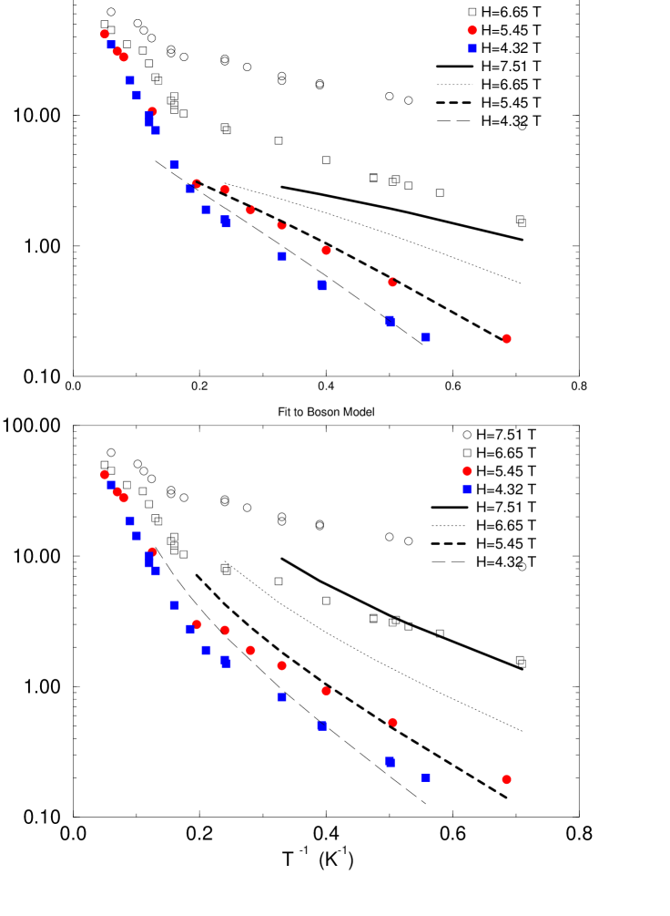
Figure 5.8: Theoretical (lines) vs. experimental data (circles and squares)

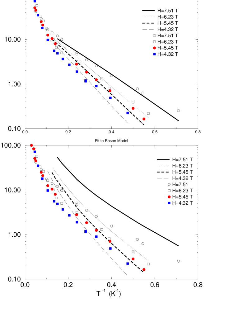
Figure 5.9: Theoretical (lines) vs. experimental data (circles and squares)

In producing these fits we get different values for $A_{w}$, the hyperfine coupling for a field placed along the $w$-direction:

$$A_{b}\sim\left\{\begin{array}[]{cc}8.5\;\;\;\mbox{MH}z&\mbox{fermions}\\ 7.0\;\;\;\mbox{MH}z&\mbox{bosons}\end{array}\right.$$ (5.23)

$$A_{c}\sim\left\{\begin{array}[]{cc}17.7\;\;\;\mbox{MH}z&\mbox{fermions}\\ 12.0\;\;\;\mbox{MH}z&\mbox{bosons}\end{array}\right.$$ (5.26)

These values are reasonable for dipolar hyperfine couplings between a nuclear spin ($s=1/2$) and the $Ni$ spin at a distance of about 2$\AA$:

$$A\sim\frac{\mu_{N}\mu_{B}}{r^{3}}\sim 2\mbox{ MH}z$$ (5.27)

Also, we can get a similar feeling for the size of the hyperfine couplings from Knight shift [51] and magnetic susceptibility [44] data for a field placed along the $b$-axis.

$$\mu_{N}\delta H\sim A\mu_{b}\chi_{s}H$$ (5.28)

At about 4K, the susceptibility is roughly a fourteenth of its maximum value. Given that $\chi_{\mbox{Max}}\sim 1/J$, and that the Knight shift at large fields is about $10^{-3}$, we get $A\sim 8$ MH$z$. It should be noted, however, that these are order of magnitude estimates; an accurate evaluation of the hyperfine matrix elements is still unavailable. Overall, the fermion fit is the better of the two. This is more obvious at high fields when the anisotropy $\Delta_{1}-\Delta_{2}$ is high (ie. when the field is along the $c$-axis). For both models, the fit to the $H\|b$ data becomes progressively worse as the field is increased. Fitting to the lower field data seems to give better overall agreement than fitting to the higher field results. This is not the case for the $h\|c$ data (at least with the fermions). Since the field in the experiment was not actually placed along the chain $c$-axis, we might expect even worse agreement between this set of data and our calculations! In fact, as mentioned before, we expect a very weak field dependence for the $h\|b$ data which would result from being close to $U(1)$ symmetry. This was the universal result of Chapter 3.

As is evident from the figures, the slope of the $h\|b$ data and the calculated results agree. This implies that the relaxation is largely mediated through thermal bosons and that the calculation is off by a $T$-independent multiplicative factor. For small anisotropy, $h\gg E$, this effect cannot come from the matrix elements for the transition or the density of states. We believe that we have taken account of the obvious mechanisms for relaxation. Terms coming from the structural properties of NENP into the Hamiltonian (as discussed in the last section) are too small to be responsible for such a large increase in the relaxation at the mid-field range. Moreover, they would be expected to play a similar role when the field is placed along the $c$-axis. There are 16 protons in the chelate surrounding each $Ni$ ion. Nuclear dipole-dipole interactions among them are energetically negligible, and thus could not be the cause for the increase in relaxation. It is certainly conceivable that the averaged hyperfine coupling is highly anisotropic, but it’s hard to explain why there would an additional dependence on the magnitude of the field. Perhaps the discrepancy is due to reasons intrinsic to the experiment.

Next we attempt to fit to the low field measurements taken for field along the $b$-axis. We find that for fields less than 4 Tesla, it is not sufficient to consider the bulk theory alone. The relaxation rate decreases with increasing field in this regime (see Fig. 5.10).

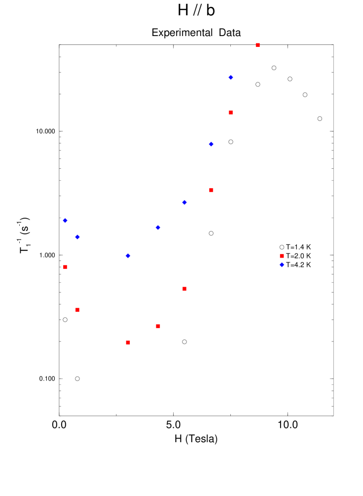
Figure 5.10: Relaxation rate for field along the $b$-axis.

We can try to apply the impurity model to explain the data. Assuming the phase shift constants, $\lambda_{\pm}^{i}$, in Eqn. (4.10) are $O(1)$, the impurity resonance width, $\Gamma$, derived in the last chapter can be graphed as in Fig. 5.11. As is clear from the plot and Eqn. (4.26), the impurity relaxation rate is essentially one delta-function peaked at $D^{\prime}/2=h$ and another peaked at $D^{\prime}/2+J^{\prime}=h$. This means that we expect two bumps in the relaxation rate due to impurity effects. The width of the bumps should correspond to the width of distribution of impurity couplings. The problem arises when we see that the temperature dependence of the low field data is roughly exponential: $\sim e^{-J^{\prime}/T}$, where the impurity coupling $J^{\prime}$ is about $4.7$K.

Figure 5.11: $\Gamma(T)$—the width of the impurity resonance

Furthermore, the sharp decrease from zero field relaxation suggests $D^{\prime}=0$. By analyzing Eqn. (4.26) we see that the second bump should have little temperature dependence. This means that assuming the first bump sits near $h=0$, the second must be larger and separated by about 3.5T. This is clearly not the case. Indeed, we would need a complicated distribution of couplings, $J^{\prime}$ and $D^{\prime}$, to get a proper fit. Adding an $E$ type anisotropy will not change these conclusions. We thus do not have a satisfactory explanation for the low field behaviour. One should take notice, however, that the data was taken for a field along the $b$-axis, where other problems were present at mid-field.

Finally, we would like to mention some recent NMR data collected on the 1-D $S=1$ spin chain $AgVP_{2}S_{6}$ by Takigawa et. al. [48]. This material is highly one dimensional with a large gap ($\Delta\sim 320$K) and very nearly isotropic ($\delta\sim 4$K). These characteristics make it ideal for analysis using our results. There are, however, some questions about the properties of the material which would have to be analyzed before an understanding of the NMR results is possible within the framework proposed here. The gap deduced from studies on the Vanadium atom ($\Delta\sim 410$K) conflicts significantly with those performed on the phosphorus sites and with neutron scattering data. In addition, the material has very low symmetry (corresponding to the space group $P2/a$) and very little is known about the possible small $E$ and $D$ terms in the Hamiltonian and their corresponding symmetry. There is fair qualitative agreement between the ${}^{31}P$ NMR data and our theory, and it is possible to explain some of the discrepancies using a temperature dependent anisotropic gap structure, but we feel that not enough is yet understood about gross features of the material to justify such speculation at this time.

Chapter 6 Suggested Experiments and Curious Predictions

We finish by pointing in this final chapter towards further experimental work which could serve to both better understand $S=1$ 1DHAF’s as well as corroborate and clarify some of the issues raised in this thesis.

6.1 Experimentally Testable Conflicts Between Models

When discussing the matrix elements, $<k,a|S^{i}(0)|q,b>$, within the different models, we noticed that there were some discrepancies between predictions. We now examine this hoping to offer experiments that would resolve the issue in favour of one model or another.

We start by discussing experiments on isotropic systems. In this case, the major differences between the predictions of the models concern large $\theta$ transitions, where we recall from Chapter 2 that

$$<k,a|l^{i}(0)|q,b>=i\epsilon^{iab}G(\theta)\;\;\;\;\;\;\cosh(\theta)=-(\omega_{k}\omega_{q}-v^{2}kq)/\Delta^{2}$$ (6.1)

This is especially dramatic in the case of backscattering. The problem with an experiment which probes large $\theta$ transitions is that contributions from matrix elements of the staggered part of the spin may be large as well. This can be cured by looking for a low temperature experiment ($T\ll\Delta$), where the energy exchanged with the probe is small. As shown in the analysis of $1/T_{1}$, the staggered contributions will be suppressed by a double Boltzmann factor, $e^{-2\Delta/T}$. A good candidate for such an experiment is elastic neutron scattering at zero or near zero magnetic field. The cross section is proportional to the spin correlation function; for elastic scattering, this is

$${\cal S}(Q,0)\propto\sum_{n,m}|<n|\mbox{ {\boldmath$\vec{S}$}}(0)|m>|^{2}\delta(\omega_{n}-\omega_{m})\delta(Q-k_{n}+k_{m})e^{-\omega_{m}/T}$$ (6.2)

At sufficiently low temperatures, this expression is simpler than the analogous one for the relaxation rate thanks to the momentum conserving delta function. The energy conserving delta function ensures that only backscattering will contribute to the cross section. Using the results of Chapter 3 we easily integrate this to give

$${\cal S}(Q,0)\propto|G(\theta)|^{2}\frac{2\omega_{Q/2}}{vQ}e^{-\omega_{Q/2}/T}$$ (6.3)

The NL$\sigma$ model gives

$$|G(\theta)|^{2}=\frac{\pi^{4}}{64}\frac{|1+(\theta/\pi)^{2}|}{|1+(\theta/2\pi)^{2}|}\left|\frac{\tanh(\theta/2)}{\theta/2}\right|$$ (6.4)

At large $Q$ this will behave as $1/\log^{2}(vQ/\Delta)$. This is very different from the free boson prediction of $G(\theta)=1$, and from the free fermion prediction of $G(\theta)\rightarrow\Delta^{2}/(vQ)^{2}$ for large $Q$. We need to qualify what we mean by ‘large’ $Q$. As discussed in Chapter 1, the field theoretic models introduced are expected to be accurate only for $Q$ near zero and $\pi$. If we want to explore the two magnon nature of the structure function, we must be near $Q\sim 0$. What we mean by ‘large’ momentum elastic scattering is the investigation of the structure function near the border region where the field theories begin to diverge from numerical simulations [16]; a region which satisfies all the criterion is $.2\pi\leq Q\leq.4\pi$. This corresponds to energies three to six times that of the gap. We expect that the differences between the models should be discernible in this range. The reason we suggest the experiment be done at zero or nearly zero magnetic field is to ensure that only backscattering transitions contribute. For nonzero field, interbranch transitions can occur at large momentum which will not necessarily select only backscattering events. This will not serve to make the interpretation transparent. The condition for backscattering even in the presence of a magnetic field is

$$Q\gg h/v$$ (6.5)

In the case of axial symmetry, we can suggest the same technique to investigate the difference between the zero field predictions of the boson and fermion models. Regardless of the size of $D$, if one only considers the cross section for scattering with $Qv>J$, then the fermion model predicts a result that vanishes as $\sim\frac{e^{-Qv/T}}{Q^{2}}$ while the boson model prediction only involves the exponential factor. The same comments apply to the case where axial symmetry is broken as well. This is no surprise since at large enough momentum, $O(3)$ symmetry is effectively restored.

Elastic neutron scattering is a good probe for the matrix elements involving large momentum and small energy exchange. Other techniques which explore the opposite regime are electron spin resonance (ESR) or far infrared absorption experiments. In both, one subjects the magnetic system to an external source of electromagnetic radiation (the microwave frequency value of the radiation depends on the transitions one is interested in investigating). The RF field couples to the spins in the same way that a magnetic field does, assuming that the electric dipole moment of the electrons on the magnetic ion is much smaller than the effective spins. The interaction Hamiltonian is therefore

$$H_{I}=\mbox{ {\boldmath$\vec{H}$}}_{\mbox{RF}}\mbox{\boldmath$G$}\cdot\sum_{i}\mbox{ {\boldmath$\vec{S}$}}_{i}\cos(\omega t)$$ (6.6)

Since the coupling is to the total spin of the system, the resonant transitions implied by Fermi’s Golden Rule will involve energy $\omega$ and zero momentum exchange. At low temperatures, the power absorbed when a uniform field is applied to the system will be

$$I(\omega)\propto\sum_{n,m}|<n|S^{i}_{q=0}|m>|^{2}\delta(\omega_{n}(h)-\omega_{m}(h)-\omega)\delta(k_{n}-k_{m})e^{-\omega_{m}/T}$$

$$\approx|<a;k,\omega_{k}^{a}(h)|S^{i}_{q=0}|b;k,\omega^{b}_{k}(h)>|^{2}e^{-\omega_{k}^{b}/T}\left|\frac{\partial(\omega^{a}_{k}(h)-\omega^{b}_{k}(h))}{\partial k}\right|^{-1}$$ (6.7)

where $a$ and $b$ denote one magnon states and $k$ satisfies, $\omega_{k}^{a}(h)-\omega_{k}^{b}(h)=\omega$. Since the density of states factor in the above is divergent for $k=0$, it stands that $I(\omega)$ will have a peak at the value of $h$ for which $\Delta^{a}(h)-\Delta^{b}(h)=\omega$. (The divergence will be cured by higher dimensional effects as discussed previously.) In a typical experiment, one judiciously chooses the RF frequency, $\omega$, to be in the vicinity of desirable transitions, and the uniform field is then tuned to the peak in the absorption power. This is much easier to do than to fine tune the RF field.

Let us now relate the ESR matrix elements to $\mbox{ {\boldmath$\vec{l}$}}_{a,b}(0,0)$, calculated in Chapter 2.

$$<a;0|S^{i}_{Q=0}|b;0>=\int dx<a;0|S^{i}(x)|b;0>=\int dx<a;0|e^{iPx}S^{i}(0)e^{-iPx}|b;0>$$

$$=\int dx<a;0|S^{i}(0)|b;0>\approx Ll^{i}_{a,b}(0,0)$$ (6.8)

Interesting conflicts between the models can be seen when there is some kind of, preferably large, anisotropy. For example, considering axial symmetry with a large $D$ anisotropy,

$$|l^{+}_{0,-}(0,0)|^{2}=\left\{\begin{array}[]{cc}\frac{1}{2}(\Delta_{3}/\Delta_{\perp}+\Delta_{\perp}/\Delta_{3}+2)&\mbox{Bosons}\\ 2&\mbox{Fermions}\end{array}\right.$$ (6.11)

The maximal difference corresponds to $\Delta_{3}/\Delta_{\perp}\sim 2$ which leads to a discrepancy of about 13% between the models. The closer the two branches lie, the better the agreement between the models. This suggests the following experiment on highly anisotropic materials (NENP being a prime candidate). One chooses two RF frequencies. The first should correspond to the large interbranch gap, $D$, and the peak absorption ought to be measured with a low field placed along the direction of the $D$ anisotropy. The second RF frequency should be $O(E)$ if the material breaks axial symmetry, or $O(h)$ if the material is axially symmetric. This should then be used to measure the absorbed ESR power with the positions of the uniform and RF fields exchanged. This second transition will involve matrix elements which will be gap independent in both models. The matrix elements from the first transition can be extracted and compared to that of the first. If the boson model is a better description even at these low fields, then the two matrix elements should be identical.

One may argue that it is redundant to make both measurements since, if the gaps are known, Eqn. (6.7) should give the correct description. The problem lies in cutting off the infrared divergence at the absorption peak. This will introduce an unknown proportionality constant. This divides out when comparing the two measurements. The ratio of the two measurements would be

$$\frac{I(\omega_{1})}{I(\omega_{2})}=\frac{1-e^{-\omega_{1}/T}}{1-e^{-\omega_{2}/T}}\frac{\Delta_{3}}{4\Delta_{\perp}}\left|l^{+}_{0,-}(0,0)\right|^{2}$$ (6.12)

where we assume a small field, $h\ll\Delta_{\perp}$, and small $E\ll D$.

To end this section, while on the subject of ESR experiments, we would like to propose additional experiments to test the impurity model presented in Chapter 4. ESR is ideal for such tests. Used in conjunction with $T^{-1}_{1}$ measurements on a given sample, it would be possible to characterize the couplings $J^{\prime}$ and $D^{\prime}$ of the end spins .

6.2 Measuring Small Anisotropies

Recall that we expect a peak in $T^{-1}_{1}$ whenever two branches cross. Experiments on Haldane Gap materials have yet to look for these. The sharpness of this peak depends on the interchain couplings which cut off the diverging integral in the calculation of the relaxation rate. Often, this will be broad because intrabranch transitions will share the same cutoff (ie. when $J_{I}>\omega_{N}$). However, the bump should be experimentally observable. We propose that information about the anisotropy tensor can be extracted from this phenomenon. Essentially, one looks for the lowest field at which this bump occurs. This would give the direction of the lowest branch and the size of the anisotropy. We now explain this further.

We assume the material in question has a well resolved $D$ anisotropy and a seemingly degenerate doublet unresolved by other experimental techniques, such as neutron scattering. One begins by placing a uniform magnetic field in the plane perpendicular to the axial direction (ie. somewhere in the $xy$-plane). The magnitude of the field should be $h^{2}>\bar{\delta}(\Delta_{3}-\Delta_{perp})$, where $\bar{\delta}$ is the uncertainty in resolving the doublet. One then proceeds to measure $T^{-1}_{1}$ for different angles in the $xy$-plane spanning a region of at most $180^{\circ}$. If there is an $E$ type anisotropy, one ought to see some structure to the data as a function of angle. Moreover, if there is such structure, we expect a bump at the angle where the branches cross. Once this angle is found, the experiment is repeated for somewhat lower field. The angle where the new bump should be seen would be greater than the old. There is actually enough information in these two measurements already to determine the anisotropy tensor. The dispersion relations are a function of the angle of the field (relative to some axis), the field magnitude and the gaps. The only unknowns are the absolute angle (or location of the axes of the anisotropy tensor) and the difference in gaps, $|\Delta_{x}-\Delta_{y}|$. The two measurements could be used to solve for these two unknowns.

In principle, one could also continue lowering the field and looking for the bump angle until it’s clear that signal is being lost when the field is reduced further. At this point, one has located the minimum crossing field which must lie along the direction associated with the middle gap. This field also gives the anisotropy: $|\Delta_{x}-\Delta_{y}|=h^{2}/|\Delta_{D}-\Delta|$.

It would be interesting to perform such an experiment on NENP. Presumably, one would find two angles corresponding to the two inequivalent chains in each unit cell. Moreover, one would be able to verify the claims made in the last chapter regarding the positions of the local anisotropy tensor in NENP.

6.3 ESR for NENP

In the last chapter we noted that NENP has two inequivalent chains per unit cell. Furthermore, their local anisotropy tensor was argued to have symmetry axes which did not correspond to the crystal axes. These facts have important ramifications for ESR experiments on NENP. Figure 6.1 shows the dispersions for chains 1 and 2 (bold and light lines, respectively) when the field is $\pi/3$ from the crystallographic $c$ axis in the $ac$-plane.

Figure 6.1: Dispersions for the two chain conformations and sample resonant transitions for a uniform field placed $60^{\circ}$ from the crystallographic $c$-axis.

This is an example of how transitions at two field strengths ought to be possible in the ESR experiment.

Figure 6.2 shows the resonance field versus orientation of field in the crystallographic $ac$-plane.

Figure 6.2: Resonant field vs. field orientation in the $ac$-plane for .19 meV transitions.

The lower branch denotes transitions in chain 1 while the upper branch corresponds to transitions in chain 2. The transitions were calculated at .19 meV. corresponding to 47 GHz. In addition the experimental results of Date and Kindo [49] are represented by the circles. One immediately sees that the data does not compare well with the predictions based on the models we’ve used so far, for instead of following one of the branches, the experimental results lie between them. Furthermore, it seems unlikely that perturbations will cause such a significant shift in the resonance field. One sees that the discrepancy is $\sim\pm 1$ Tesla. One possible explanation is that since the ESR signal in [49] was also $\sim\pm 1$ Tesla in width and symmetric (in conflict with the predictions of [47]), the signal from the resonances in both chains was somehow smeared and interpreted as one single peak. Seen that way the model predictions are in good agreement except for the large field regime. One also has to keep in mind that the high-field boson dispersions are not accurate and therefore the predictions at larger angles could easily be .5 Tesla (or more) off the mark. We propose that further ESR experiments be done on NENP which specifically look for the double resonance predicted here.

To end this discussion, we’d like to elaborate on a previously made statement regarding the assignment of masses to the local Ni symmetry axes. It’s easy to see that switching the masses around is tantamount to a $\pi/2$ shift in Figure 5.2 (the fact that the gyromagnetic constants are not the same in orthogonal directions will not change the ESR resonance graph much since the ratio of the gyromagnetic constants is 0.98). Redrawing Figure 6.2 with this geometry misses the experimental results by 4 Tesla at 0 and 90 degrees, where the two chain resonances coincide. This determines the proper labeling of the local symmetry axes.

Chapter 7 Concluding Remarks

Jacob. S. Sagi

With the increasing theoretical interest in low dimensional systems, there has been a proportionate increase in the number of both realizable physical systems and experiments. This work offers a comprehensive analysis of NMR relaxation in Haldane gap materials, taking account of anisotropy and other material properties. As well, our analysis has led to predictions pertaining to other types of experiments. It is hoped that our efforts will aid in both extending and clarifying existing knowledge of the subject.

References

- [1] F.D.M. Haldane, Phys. Lett. 93A, 464 (1983). For a review see I. Affleck, J. Phys.:Condensed Matter 1, 2047 (1989).
- [2] See C. Kittel, Quantum Theory of Solids (Wiley, New York, 1963) Ch. 4, for a review.
- [3] P.W. Anderson in Solid State Physics, ed. F. Seitz and D. Turnbull (Academic Press, New York, 1963) Vol. 14, p. 99.
- [4] See A. Abragam and B. Bleaney, EPR of Transition Ions (Claredon Press, Oxford, 1970).
- [5] S. Coleman, Comm. Math. Phys. 31, (1973) 259.
- [6] For details and more references see I. Affleck, Fields, Strings and Critical Phenomena, ed. E. Brézin and J. Zinn-Justin (North-Holland, Amsterdam, 1990), p. 563.
- [7] F.D.M. Haldane, Phys. Rev. Lett. 61, 1029 (1988).
- [8] E. Fradkin and M. Stone, Phys. Rev. B 38, 7215 (1988).
- [9] P.W. Atkins and J.C. Dobson, Proc. Roy. Soc. A 321, 321 (1971); J.M. Radcliffe, J. Phys. A 4, 313 (1971); A.M. Perelomov, Commun. Math. Phys. 20, 222 (1972).
- [10] A.M. Polyakov, Gauge Fields and Strings (Harwood Academic Publishers, London, 1987) Ch. 8.
- [11] A.B. Zamolodchikov and A.B. Zamolodchikov, Ann. Phys. 120, 253 (1979).
- [12] M. Karowski and P. Weisz, Nuc. Phys. B139, 455 (1978)
- [13] R. Botet and R. Julien, Phys. Rev. B 27, 613 (1983); R. Botet, R. Julien and M. Kolb, Phys. Rev. B 28, 3914 (1983); M. Kolb, R. Botet and R. Julien, J. Phys. A 16, L673 (1983); M.P. Nightingale and H.W.J. Blöte, Phys. Rev. B 33, 659 (1986); H.J. Schultz and T.A.L. Ziman, Phys. Rev. B 33, 6545 (1986).
- [14] S.R. White and D.A. Huse, Phys. Rev. B 48, 3844 (1993).
- [15] O. Golinelli, Th. Jolicœur and R. Lacaze, Phys. Rev. B 50, 3037 (1994).
- [16] E.S. Sørensen and I. Affleck, Phys. Rev. Lett. 71, 1633 (1993).
- [17] S. Ma, C. Broholm, D.H. Reich, B.J. Sternlieb and R.W. Erwin, Phys. Rev. Lett. 69, 3571 (1992).
- [18] D.V. Khveshchenko and A.V. Chubukov, Sov. Phys. JETP 66, 1088 (1987).
- [19] I. Affleck and R.A. Weston, Phys. Rev. B 45, 4667 (1992).
- [20] I. Affleck, Phys. Rev. Lett. 62, 474 (1989).
- [21] A.M. Tsvelik, Phys. Rev. B 42, 10499 (1990).
- [22] I. Affleck, Phys. Rev. Lett. 56, 746 (1986).
- [23] For details and more references see P. Ginsparg, Fields, Strings and Critical Phenomena, ed. E. Brézin and J. Zinn-Justin (North-Holland, Amsterdam, 1990).
- [24] C. Itzykson and J.C. Drouffe, Statistical Field Theory: Vol 2 (Cambridge University Press, Cambridge, 1989) Ch. 2.3.
- [25] A.B. Zamolodchikov and V.A. Fateev, Sov. J. Nucl. Phys. 43, 657 (1986).
- [26] I. Affleck and F.D.M. Haldane, Phys. Rev. B 36, 5291 (1987).
- [27] T.T. Wu, B. McCoy, C.A. Tracy and E. Barouch, Phys. Rev. B 13, 316 (1976).
- [28] R. Kubo and K. Tomita, J. Phys. Soc. Jap. 9, 888 (1954); T. Moriya, Progr. Theoret. Phys. (Kyoto) 16, 23 (1956).
- [29] Th. Jolicoeur and O. Golinelli, Phys. Rev. B 50, 9265, (1994).
- [30] H.J. Schulz, Phys. Rev. B 34, 6372 (1986).
- [31] Jean-Paul Blaizot and Georges Ripka, Quantum Theory of Finite Systems (MIT Press, 1986), Chapter 3.
- [32] P.P. Mitra and B.I. Halperin, Phys. Rev. Lett. 72, 912, (1994).
- [33] I. Affleck, Phys. Rev. B 43, 3215 (1991).
- [34] N. Fujiwara, T. Goto, Satoru Maegawa and Toshiro Kohomoto, Phys. Rev. B 47, 11860 (1993).
- [35] M. Troyer, H. Tsunetsugu and D. Wurtz, Phys. Rev. B 50, 13515 (1994).
- [36] G.D. Mahan, Many Particle Physics (Plenum Press, 1993), p. 604.
- [37] J.L. Cardy, Nuc. Phys. B270, 186 (1986).
- [38] F.D.M. Haldane, Phys. Rev. Lett. 47, 1840 (1981).
- [39] I. Affleck, T. Kennedy, E.H. Lieb and H. Tasaki, Phys. Rev. Lett. 59, 799 (1987); Commun. Mat. Phys. 115, 477 (1988).
- [40] T. Kennedy, J. Phys. Con. Matt. 2, 5737 (1990); S.M. Girvin and D.P. Arovas, Phys. Scr. T27, 156 (1989); M. Hagiwara, K. Katsumata, I. Affleck, B.I. Halperin and J.P. Renard, Phys. Rev. Lett. 65, 3181 (1990); S.H. Glarum, S. Geschwind, K.M. Lee, M.L. Kaplan and J. Michel, Phys. Rev. Lett. 67, 1614 (1991).
- [41] S. White, Phys. Rev. Lett. 69, 2863 (1992).
- [42] E.S. Sørensen and I. Affleck, Phys. Rev. B 51, 16115 (1995).
- [43] P.P. Mitra, B.I. Halperin and I. Affleck, Phys. Rev. B 45, 5299 (1992).
- [44] J.P. Renard, M. Verdaguer, L.P. Regnault, W.A.C. Erkelens, J. Rossat-Mignod, J. Ribas, W.G. Stirling and C. Vettier, J. Appl. Phys. 63, 3538 (1988).
- [45] A. Meyer, A. Gleizes, J.J. Girerd, M. Verdaguer and O. Kahn, Inorg. Chem. 21, 1729 (1982).
- [46] T. Sakai and H. Shiba, Proceedings of ISSP Symposium on Frontiers in High Magnetic Fields (Tokyo, Nov. 10-12, 1993).
- [47] I. Affleck, Phys. Rev. B 46, 9002 (1992).
- [48] M. Takigawa, T. Asano, M. Mekata, Y. Ajiro, E.T. Ahrens and Y.J. Uemura, Preprint.
- [49] M. Date and K. Kindo, Phys. Rev. Lett. 65, 1659 (1990).
- [50] I. Affleck, Phys. Rev. B 41, 6697 (1990).
- [51] M. Chiba, Y. Ajiro, H. Kikuchi, T. Kubo and T. Morimoto, J. Mag. and Mag. Mat. 90 & 91 221 (1990).