GENERALIZED HELIMAGNETS BETWEEN TWO AND FOUR DIMENSIONS

Abstract

We study the phase transitions of N-components generalized helimagnets that obey the symmetry breaking pattern ${\rm O}(N)\times{\rm O}(N-1)\rightarrow{\rm O}(N-1)_{\rm diag}$. In the neighborhood of two dimensions, a $D=2+\epsilon$ renormalization group study reveals a rich fixed point structure as well as a nematic-like phase with partial spin ordering. In the physical case ${\rm O}(3)\times{\rm O}(2)\rightarrow{\rm O}(2)_{\rm diag}$, relevant to real magnets with noncollinear ordering, we show that this implies an XY-like transition between the ordered phase and the nematic-like phase. A non-Abelian mean-field calculation qualitatively valid above four dimensions is shown to lead to the same picture but then the principal chiral fixed point, which had been proposed earlier as the relevant fixed point for D=3 helimagnets, plays no role due to the appearance of a first-order line.

Several physical systems display a peculiar critical behaviour associated with helical or noncollinear ordering. These include helimagnets, the dipole-locked phase of superfluid Helium as well as Josephson junction arrays in a transverse magnetic field[1]. A prototypical example is the stacked triangular lattice antiferromagnet (STA) whose low-temperature ordered phase breaks completely the rotation symmetry group. When generalized to N-component spins, the Landau-Ginzburg free energy for this system contains two quartic invariants:

$$H= {1\over 2}\left({\left({\nabla\vec{\varphi}_{1}}\right)^{2}+\left({\nabla\vec{\varphi}_{2}}\right)^{2}}\right)+r\left({\vec{\varphi}_{1}^{2}+\vec{\varphi}_{2}^{2}}\right)$$ (2)

$$+u\left({\vec{\varphi}_{1}^{2}+\vec{\varphi}_{2}^{2}}\right)^{2}+v\left({\left({\vec{\varphi}_{1}\cdot\vec{\varphi}_{2}}\right)^{2}-\vec{\varphi}_{1}^{2}\,\vec{\varphi}_{2}^{2}}\right).$$

When $u,v>0$, this free energy describes a second-order phase transition between a high-temperature phase which is ${\rm O}(N)\times{\rm O}(2)$-symmetric and a low-temperature phase with lower symmetry ${\rm O}(N-2)\times{\rm O}(2)_{\rm diag}$. This theory has been studied in the neighborhood of four dimensions by the standard $\epsilon$-expansion[2, 3]. The main point of these studies is that when the number of components is large enough there is a fixed point with $u^{*},v^{*}\neq 0$ that describes a critical behaviour different from the well-studied behaviour of the N-vector model. In the neighborhood of the upper critical dimension, D=4, there is a dividing line $N_{c}(D)=21.8-23.4\epsilon+O(\epsilon^{2})$ in the (N, D)-plane above which there is a second-order phase transition and below which there is a fluctuation-induced first-order transition (no stable fixed point). This is similar to the case of the normal-superconducting phase transition[4]. The fate of the line $N_{c}(D)$ is not known outside the $\epsilon$-expansion. Numerical studies on the STA lattice (thus in D=3) have shown that the ordering transition is second-order with exponents that do not belong to the ${\rm O}(N)$ Wilson-Fisher universality classes[5, 6, 7], $\nu=0.585(9)$, $\gamma/\nu=2.011(14)$[6]. These exponents are also observed in the body-centered tetragonal antiferromagnet[8], suggestive of a new universality class, usually called chiral universality class. It has been suggested[3, 5, 9] that these exponents are ruled by the nontrivial fixed point which exists for $N>N_{c}(D)$.

The study of these phenomena has been also performed from the low-temperature expansion. A non-linear sigma model that captures the Goldstone modes of the theory has been constructed by Dombre and Read[10]. It involves an order parameter which is a rotation matrix instead of a vector as in usual magnetic systems. This is due to the fact that the rotation group is fully broken in the low-temperature phase of noncollinear magnets. The symmetry breaking pattern is ${\rm SO}(3)\times{\rm SO}(2)\rightarrow{\rm SO}(2)_{\rm diag}$ where the internal ${\rm SO}(2)$ rotation acts upon the 1,2 indices of the fields of Eq.(2). We can parametrize the rotation matrix of the non-linear sigma model by three orthogonal unit vectors ${\vec{\phi}}_{1},{\vec{\phi}}_{2},{\vec{\phi}}_{3}$ and the Euclidean action can be then written as:

$$S=\int\!d^{D}x\,{1\over 2g_{1}}\left((\nabla{\vec{\phi}}_{1})^{2}+(\nabla{\vec{\phi}}_{2})^{2}\right)+{1\over 2g_{2}}(\nabla{\vec{\phi}}_{3})^{2}.$$ (3)

The STA corresponds to a bare value $1/g_{2}=0$. The renormalization group flow of the two couplings $g_{1},g_{2}$ has been studied[11] in a $D=2+\epsilon$ expansion. It has been noted that a remarkable symmetry enhancement happens on the line $g_{1}=g_{2}$. In this case the global symmetry of Eq. (3) is ${\rm SO}(3)\times{\rm SO}(3)$ broken down to the diagonal subgroup ${\rm SO}(3)$. This is the so-called principal chiral model which is renormalizable and thus the peculiar line $g_{1}=g_{2}$ is stable under the RG flow. Since ${\rm SO}(3)\times{\rm SO}(3)\equiv{\rm SO}(4)$, this line is described by the usual ${\rm SO}(4)$ sigma model, at least within the $D=2+\epsilon$ expansion. Since this fixed point is stable and has an exponent $\nu\approx 0.74$ there is a clear conflict with numerical and experimental findings in $D=3$.

In this Letter we shed new light on this problem by studying a new generalization to N components of this sigma model as well as by a non-Abelian mean-field calculation. We show that the sigma model has a much richer structure than previously expected and we propose a scenario in which the principal chiral fixed point with ${\rm SO}(4)$ symmetry plays no role in $D=3$ due to the appearance of a first-order transition.

In the two-dimensional case, the perturbative beta functions[12, 11] indicate a flow which is infrared unstable away from the origin $g_{1}=g_{2}=0$ but the whole line $g_{2}=0$ is a line of unstable fixed points as can read from the RG formulas. This fact has a simple interpretation: when $g_{2}\rightarrow 0$ the vector ${\vec{\phi}}_{3}$ becomes frozen and the remaining degrees of freedom are simply the rotations of the vectors ${\vec{\phi}}_{1},{\vec{\phi}}_{2}$ in the plane orthogonal to ${\vec{\phi}}_{3}$. Since ${\vec{\phi}}_{1}$ and ${\vec{\phi}}_{2}$ are themselves orthogonal, we are left with an XY model whose coupling is $g_{1}$. The corresponding beta function is zero in perturbation theory. However it is important to note that in $D=2$ this XY model will undergo the Kosterlitz-Thouless (KT) transition for a finite value of $g_{1}$. This phenomenon is not seen in perturbation theory and is not found in the perturbative beta functions. We expect that the line of fixed points $g_{2}=0$ will end at some critical value. Above this value, the flow will go to the high-temperature fixed point in the disordered phase of the XY model. This transition is the unbinding transition of the vortices of the XY model. If we unfreeze the vector ${\vec{\phi}}_{3}$ by setting $g_{2}\neq 0$, then topological defects survive because, as noted by Kawamura and Miyashita[13], $\Pi_{1}({\rm SO}(3))=Z_{2}$. All XY vortices with even winding number become topologically trivial while those with odd winding number become all equivalent and nontrivial.

To complete the phase diagram in the ($g_{1}-g_{2}$)-plane, we note that for $g_{1}=\infty$ the model (3) becomes the ${\rm O}(3)$ sigma model which has no transition in D=2: the coupling $g_{2}$ flows continuously to the high-temperature fixed point. If we assume that there are no other fixed points, we are led to propose the phase diagram shown in Fig. 1. This means that for nonzero values of the couplings the model is always disordered and there is no phase transition at nonzero temperature as expected for a system with non-abelian symmetry.

We note that the KT point on the $g_{1}$ axis cannot be studied by extending the model simply to $N$ components. The low-temperature limit of the theory (1) is an ${\rm O}(N)\times{\rm O}(2)$ sigma model[14] that has also two coupling constants. The corresponding phase diagram is topologically similar to Fig. 1: the KT point remains at finite coupling unreachable by perturbation theory.

To clarify the situation, we will study another generalization of the ${\rm O}(3)\times{\rm O}(2)$ model which involves $N$ orthogonal unit vectors with $N$ components ${\vec{\phi}_{1}},\dots,{\vec{\phi}_{N}}$ and the action is:

$$S=\!\int\!d^{D}\!x{1\over 2g_{1}}\left((\nabla{\vec{\phi}}_{1})^{2}\!+\dots+(\nabla{\vec{\phi}}_{N-1})^{2}\right)+{1\over 2g_{2}}(\nabla{\vec{\phi}}_{N})^{2}.$$ (4)

The symmetry breaking pattern is now ${\rm SO}(N)\times{\rm SO}(N-1)\rightarrow{\rm SO}(N-1)_{\rm diag}$. This is a sigma model which is defined on a space which is homogeneous but not maximally symmetric. When $g_{1}=g_{2}$, one is dealing with the sigma model defined by the maximally symmetric space ${\rm SO}(N)\times{\rm SO}(N)/{\rm SO}(N)_{\rm diag}$, this is the so-called principal chiral model. When $g_{2}\rightarrow 0$, it reduces to the principal chiral ${\rm SO}(N-1)$ model, and when $g_{1}\rightarrow\infty$ to the ${\rm O}(N)$ vector model. In fact, this model has been studied some time ago by Friedan[12] who has shown that it is renormalizable in two dimensions with only two coupling constants. The corresponding RG flow in $D=2+\epsilon$ is depicted in Fig. 2.

The principal chiral models are known to have a fixed point within the $D=2+\epsilon$ expansion: these are the points C_N and C_N-1 in Fig. 2. The ${\rm O}(N)$ vector model has also a fixed point O_N which is at distance $\epsilon$ from the upper left-hand corner of the Fig. 2. The novelty is that we find a fixed point P_N with nontrivial values of the couplings $g_{1},g_{2}$ which is not on the diagonal $g_{1}=g_{2}$. This fixed point has two directions of instability and thus there are two phase transition lines: one that goes from P_N to O_N and one that goes from P_N to C_N-1. This implies that there is an intermediate phase in addition to the high-temperature paramagnetic phase and the low-temperature ordered phase. In this new phase, the vector ${\vec{\phi}}_{N}$ is ordered because it is in the low-temperature regime of the ${\rm O}(N)$ model but the remaining $N-1$ vectors ${\vec{\phi}}_{1},\dots,{\vec{\phi}}_{N-1}$ are still fluctuating in the subspace orthogonal to ${\vec{\phi}}_{N}$. Due to this partial ordering, we will refer to this phase as “nematic”. The transition between the fully ordered phase and the nematic phase is governed by the fixed point C_N-1 and the transition between nematic and paramagnetic phases by the ${\rm O}(N)$ fixed point. The fixed point C_N which has the highest symmetry governs the critical behaviour of the direct transition between the paramagnetic phase and the fully ordered phase.

This phase diagram thus points to a possible explanation of what happens in the ${\rm O}(N)\times O(2)$ sigma model above two dimensions. Here the point C_N-1 is replaced by an ${\rm O}(2)$ point which is not seen in the $D=2+\epsilon$ expansion. This point is located at $g_{2}=0$ but $g_{1}=O(1)$ and thus the perturbative flow of the coupling $g_{1}$ is that of a low-temperature phase. The O$(3)$ point is seen in perturbation theory[15]. The mixed fixed point will also be invisible in perturbation theory. In fact, in the flow equations of the generalized model, the limit $N\rightarrow 3$ leads to $g^{*}_{1}\rightarrow\infty$ and $g^{*}_{2}=O(\epsilon)$. When $D\rightarrow 2$ the fixed points that were of order $\epsilon$ collapse to the origin but the ${\rm O}(2)$ fixed point becomes the KT point at the end of a line of perturbative fixed points. So the picture we have constructed leads naturally to a phase diagram as Fig. 1 for all ${\rm O}(N)\times{\rm O}(2)$ models.

These $D=2+\epsilon$ expansion results clearly show that the phase diagrams of the these sigma models is much more complex than previously thought[11]. Notably the fixed point P_N is a prominent candidate to interact with the principal chiral point C_N. To deepen our understanding, we now turn to a mean-field study of the ${\rm O}(3)\times{\rm O}(2)$ sigma model on a hypercubic lattice. This lattice model is regularized both in the ultraviolet and in the infrared limit: this is a sensible way to define the sigma model beyond perturbation theory. Note that to construct a continuum field theory one has to find a second-order phase transition which is not guaranteed a priori. We introduce a field ${\vec{\lambda}}_{i}$ conjugate to each vector ${\vec{\phi}}_{i}$ in the action (3). The standard mean-field method then involves a non-Abelian integration over the ${\rm O}(3)$ matrix $({\vec{\phi}}_{1},{\vec{\phi}}_{2},{\vec{\phi}}_{3})$. We start from the Hamiltonian:

$$H=-\sum_{<x,y>}\!K_{i}\,{\vec{\phi}}_{i}(x)\cdot{\vec{\phi}}_{i}(y)\equiv-\sum K_{i}\,{\vec{\phi}}_{i}\cdot V^{-1}\!\!\cdot{\vec{\phi}}_{i},$$ (5)

where the sum is over nearest-neighbor lattice sites, $V_{xy}$ is the connectivity matrix and we take only two distinct couplings: $K_{1}\simeq 1/g_{1}$ for ${\vec{\phi}}_{1},{\vec{\phi}}_{2}$ and $K_{2}\simeq 1/g_{2}$ for ${\vec{\phi}}_{3}$. We write the partition function as:

$$Z=\int d{\vec{\lambda}}_{i}\,{\rm e}^{-{T\over 4K_{i}}{\vec{\lambda}}_{i}\cdot V^{-1}\!\cdot{\vec{\lambda}}_{i}}\int d\mu({\vec{\phi}}_{i})\,{\rm e}^{\mathop{\Sigma}\limits_{i}{\vec{\lambda}}_{i}\cdot{\vec{\phi}}_{i}}.$$ (6)

Here $d\mu$ is the Haar measure on ${\rm SO}(3)$ and T is the temperature. The mean-field theory is obtained by a saddle-point treatment of the integral over the auxiliary fields ${\vec{\lambda}}_{i}$. We have searched spatially uniform solutions since the model (5) is ferromagnetic. There is a phase where all the expectation values $\langle{\vec{\lambda}}_{i}\rangle$ are zero: this is the high-temperature fully disordered phase and there is also a phase where all the $\langle{\vec{\lambda}}_{i}\rangle$ are non zero: this is fully ordered phase that breaks the full rotational invariance. But we also find a phase where $\langle{\vec{\lambda}}_{3}\rangle\neq 0$ but $\langle{\vec{\lambda}}_{1,2}\rangle=0$: this is the nematic phase. The corresponding phase diagram is sketched in Fig. 3.

The most remarkable feature is the appearance of a first-order line that crosses the diagonal $K_{1}=K_{2}$. Its existence is simple to understand: the non-Abelian integral in Eq.(6) has no simple closed form but its expansion in powers of group invariants built from the matrix $\Lambda=({\vec{\lambda}}_{1},{\vec{\lambda}}_{2},{\vec{\lambda}}_{3})$ is simple. Since we are dealing with the rotation group there is an odd invariant that appears in the mean-field potential: ${\rm Det}[\Lambda]$. This cubic contribution gives rise to the first-order transition (thick line in Fig. 3). This line terminates at tricritical points and is continued by second-order transition lines: in particular for $K_{2}$ small enough there is a second-order transition to the fully ordered phase. In the limiting case K${}_{2}=0$, it is not necessary to introduce the auxiliary field ${\vec{\lambda}}_{3}$ in Eq.(6) and a standard calculation leads immediately to the Landau theory in Eq.(2). When $0<K_{2}<K_{1}$, the field ${\vec{\lambda}}_{3}$ is necessarily present but it remains massive at the phase transition: At the transition the fields $\vec{\lambda}_{1},\vec{\lambda}_{2}$ get a non-zero expectation value, but the $\det[\Lambda]$ term in the potential acts as a magnetic field and immediately induces also an ordering of $\vec{\lambda}_{3}$.

The intermediate ordering transitions that occur in the $K_{2}>K_{1}$ region are second-order close to the boundaries. These lines still exist in the unphysical region below the first-order line: they are then spinodal lines and they converge right at the diagonal toward the chiral point C₃, which is thus metastable. As a consequence, we note that the latticized principal ${\rm O}(3)$ chiral model does not lead to a continuous theory: there is no place where the correlation length diverges. In fact there is numerical evidence from Monte-Carlo studies[16, 17] for a first-order transition in the model (5) at $K_{1}=K_{2}$ in three dimensions in agreement with the mean-field prediction. These studies have also obtained marginal evidence for the chiral universality class exponents of Refs.([5, 6, 7]) by simulation of (5) for the value $K_{2}=0$. This Hamiltonian is expected to be in the same universality class as the STA-type helimagnets. From our findings it is however clear that the proximity of a tricritical point as seen in mean-field theory may lead to difficulties in the observation of the true critical behaviour: indeed the first-order line begins at $K_{2}/K_{1}=8.5$.

In conclusion, we have shown the existence of a nematic phase with partial spin ordering in the family of sigma models ${\rm SO}(N)\times{\rm SO}(N-1)\rightarrow{\rm SO}(N-1)_{\rm diag}$. For $N>3$, all relevant fixed points are captured by a $D=2+\epsilon$ expansion. In the physical case SO(3)$\times$SO(2) there is an XY phase transition between the fully ordered phase and the nematic phase. We obtain a similar picture from mean-field theory with the appearance of a first-order line that continue the helimagnetic second-order line between the paramagnetic and the fully ordered phases, and isolates the principal chiral fixed point C₃ with SO(3)$\times$SO(3) symmetry in the metastability region. The simplest scenario is that this line appears at an unknown critical dimension $D_{c}$ above which the $D=2+\epsilon$ is replaced by the mean-field picture. In this respect we note that the intersection of the spinodal lines on the diagonal is suggestive of a collapse of the two fixed points P_N and C_N. If this critical dimension $D_{c}$ is between 2 and 3, there is a natural explanation to the fact that the chiral universality class has exponents different from O(4).

FIG. 1.: Global renormalization group flow of the ${\rm O}(3)\times{\rm O}(2)$ sigma model in two dimensions. The perturbative line of fixed points on the $g_{1}$ axis ends at a KT fixed point.

FIG. 2.: The RG flow and the corresponding phase diagram of the $O(N)\times O(N-1)$ sigma model in the neighborhood of two dimensions $D=2+\epsilon$. There is a high-temperature paramagnetic phase, a fully ordered phase at low temperature and an intermediate nematic-like phase where the $\phi_{N}$ vector is ordered but the other vectors are disordered. The diagonal $g_{1}=g_{2}$ is the principal chiral model.

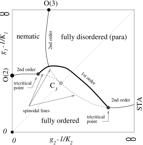
FIG. 3.: The non-Abelian mean-field phase diagram of the $O(3)\times O(2)$ sigma model (sketchy).

- [1] For a review, see M. L. Plumer, A. Caillé, A. Mailhot and H. T. Diep in “Magnetic Systems with Competing Interactions”, H. T. Diep editor, World Scientific, Singapore 1994.
- [2] T. Garel and P. Pfeuty, J. Phys. C9, L245 (1976); see also D. Bailin, A. Love and M. A. Moore, J. Phys. C10, 1159 (1977).
- [3] H. Kawamura, Phys. Rev. B38, 4916 (1988).
- [4] B. I. Halperin, T. C. Lubensky and S. K. Ma, Phys. Rev. Lett. 32, 292 (1974).
- [5] H. Kawamura, J. Phys. Soc. Jpn. 61, 1299 (1992), and references therein.
- [6] T. Bhattacharya, A. Billoire, R. Lacaze and Th. Jolicoeur, J. Phys. I (Paris) 4, 181 (1994).
- [7] D. Loison and H. T. Diep, Phys. Rev. B50, 16453 (1994).
- [8] H. T. Diep, Phys. Rev. B39, 3973 (1989).
- [9] Th. Jolicœur, Europhys. Lett. 30, 555 (1995).
- [10] T. Dombre and N. Read, Phys. Rev. B39, 6797 (1989).
- [11] P. Azaria, B. Delamotte and Th. Jolicœur, Phys. Rev. lett. 26, 3175 (1990).
- [12] D. H. Friedan, Ann. Phys. 163, 318 (1985).
- [13] H. Kawamura and S. Miyashita, J. Phys. Soc. Jpn, 53, 4138 (1984).
- [14] P. Azaria, B. Delamotte, F. Delduc and Th. Jolicœur, Nucl. Phys. B408, 485 (1993).
- [15] A. V. Chubukov, Phys. Rev. B44, 5362 (1991).
- [16] H. Kunz and G. Zumbach, J. Phys. A26, 3121 (1993).
- [17] H. T. Diep and D. Loison, J. Appl. Phys. 76, 1 (1994).