A study of fragmentation processes using a discrete element method

Abstract

We present a model of solids made from polygonal cells connected via beams. We calculate the macroscopic elastic moduli from the beam and cell parameters. This modellisation is particularly suited for the simulation of fragmentation processes. We study the effects of an explosion inside a circular disk and the impact of a projectile and obtain the fragment size distribution. We find that if breaking only happens under tensile forces a layer on the free wall opposed to impact is first ejected. In that case the distribution follows a power-law with an exponent that in most cases is around two.

Laboratoire de Physique Mécanique des Milieux Hétérogènes, C.N.R.S., U.R.A. 857

École Supérieure de Physique et Chimie Industrielle

10 rue Vauquelin, 75231 Paris, Cedex 05, France

1 Introduction

Fragmentation plays an important role in a wide variety of physical phenomena. Examples range from geophysics to astrophysics: fragments from weathering, coal heaps, rock fragments from chemical and nuclear explosions, projectile collisions, asteroids etc. Most of the measured fragment size distributions show power law behavior with exponents between 1.9 and 2.6 concentrating around 2.4 [1] - [4]. Power law behavior for small fragment masses seems to be a common characteristic of the breaking of brittle objects.

Fragmentation in one dimension was studied using thin glass rods dropped vertically onto the floor [5]. Depending on the height from which the rod was dropped the fragment size distribution varies from log - normal to power law with increasing height.

Recently, Oddershede, Dimon and Bohr reported that the mass distribution of fragments produced by impact experiments shows universal power law behavior. The scaling exponents depend on the overall morphology of the objects but are independent of the type of the material. (Their experiment was performed with several different kinds of materials, gypsum, soap, paraffin, potato.) Because of the universal power law behavior found without any control parameter, they concluded that the fragmentation process is a self - organized critical process with exponent $\sim 1.6$ [6].

Several theoretical approaches were established to describe fragmentation. In one dimensional stochastic models power law, exponential and log-normal fragment mass distributions can be obtained depending on the fracture point distributions [7].

Discrete stochastic processes have also been studied as models for fragmentation using cellular automata. In Ref. 8 two- and three - dimensional cellular automata were proposed to model power law distribution in shear experiments on a layer of uniformly sized fragments.

In Ref. 9 an iterative stochastic process is studied as a model of two- and three - dimensional discrete fragmentation. Depending on the parameters of the model, log - normal and power law distribution were found for the fragment size distribution.

The mean - field approach describes the time evolution of the concentration $c(x,t)$ of fragments having mass $x$ through a linear integro - differential equation [10]:

$$\frac{\partial c(x,t)}{\partial t}=-a(x)c(x,t)+\int_{x}^{\infty}c(y,t)a(y)f(x|y)dy$$ (1)

where $a(x)$ is the overall rate at which $x$ breaks in a time interval $dt$, while $f(x|y)$ is the relative rate at which $x$ is produced from the break-up of $y$. With some further assumptions on $f(x|y)$ exact results can be obtained but in physically interesting situations the solution is very difficult [10].

Three - dimensional impact fracture processes of random materials were modeled based on competitive growth of cracks [11]. A universal power law fragment mass distribution was found consistent with self - organized criticality with an exponent of $\frac{5}{3}$.

Recently, a two dimensional dynamic simulation of solid fracture was performed using a cellular model material [12, 13]. The compressive failure of a rectangular sample, the four - point shear failure of a beam and the impact of particles with a plate and with other particles were studied.

In this paper we present a two dimensional dynamic simulation of the fragmentation of granular materials. We establish a two - dimensional model for a deformable, breakable, granular solid by connecting unbreakable, undeformable elements with elastic beams, similar as in Refs. 12,13 . The contacts between the particles can be broken according to a certain breaking rule, which takes into account the stretching and bending of the connections. The breaking rule contains two parameters to describe the relative importance of the two breaking modes. We address the question how the fragment mass distribution depends on the breaking parameters. After measuring the macroscopic elastic behavior of our granular solid the model is applied to study fragmentation caused by an explosion inside a solid and by a projectile impact.

2 The model

In order to study the fragmentation of granular solids we use Molecular Dynamics (MD) simulations in two dimensions. A general overview of MD simulations applied to the field of granular materials can be found in Ref. 14. This method calculates the motion of particles by solving Newton’s equations. In our simulation this is done using a Predictor Corrector scheme.

Our model of a deformable, breakable granular solid is a generalization of the model which was used earlier to study the flow of granular materials [15]. The model construction is composed of three major steps, namely, the implementation of the granular structure of the solid, the determination of the elastic behavior by the contact force and the beam models, and finally the breaking of the solid. In this section, the three steps of the model construction are presented in detail.

(a) Granularity

In order to take into account the complex structure of the granular solid we use arbitrarily shaped convex polygons. To get an initial configuration of these polygons we construct a vectorizable random lattice, which is a Voronoi construction with a regularization procedure (see Ref. 16). The advantage of the vectorizable random lattice compared to the ordinary Poissonian Voronoi tessellation is that the number of neighbors of each polygon is limited which makes the computer code faster and allows to simulate larger systems. The convex polygons of this Voronoi construction are supposed to model the grains of the material, see Ref. 15. In this way the structure of the solid is built on a mesoscopic scale. Each element is thought of as a large collection of atoms. In our simulation however these polygons are the smallest particles interacting elastically with each other. All the polygons have three continuous degrees of freedom in two dimensions: the two coordinates of the positions of the center of mass and the rotation angle.

(b) Elastic behavior of the solid

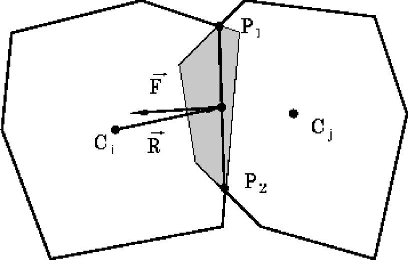
Figure 1: To calculate the elastic contact force $\vec{F}$ between two particles one has to obtain the overlap area. The intersection points $P_{1}$, $P_{2}$ define the contact line $\vec{P_{1}P_{2}}$. The force is applied at the center of the contact line $\vec{R}$ and the direction of the force is perpendicular to $\vec{P_{1}P_{2}}$.

The elastic behavior of the solid is captured in the following way: The polygons are considered to be rigid bodies. They are not breakable and not deformable. But they can overlap when they are pressed against each other representing to some extent the local deformation of the grains. Usually the overlapping polygons have two intersection points. These points define the contact line (see Fig. 1).

In order to simulate the elastic contact force between touching grains we introduce a repulsive force between the overlapping polygons. This force is proportional to the overlapping area $A$ divided by a characteristic length $L_{c}$ of the interacting polygon pair. Our choice of $L_{c}$ is given by $1/L_{c}=1/2(1/r_{i}+1/r_{j})$, where $r_{i},r_{j}$ are the diameters of circles of the same area as the polygons. This normalization is necessary in order to reflect the fact that the spring constant is proportional to the elastic modulus divided by a characteristic length. (In the case of a linear spring this characteristic length is simply the equilibrium length of the spring.) The direction of the force is chosen to be perpendicular to the contact line of the polygons.

The contact force $\vec{F}_{ij}$ between two particles is given by

$$\vec{F}_{ij}=-\frac{YA}{L_{c}}\vec{n}$$ (2)

where $\vec{n}$ is the unit vector perpendicular to the contact line (see Fig. 1) and $Y$ is the grain bulk Young modulus. The friction of the touching polygons can be implemented according to Coulomb’s friction law (see also Ref. 15). However it turned out from the simulations that friction does not play an important role in the fragmentation of the granular solids. Therefore, in the present simulations the friction term was omitted.

In order to keep the solid together it is necessary to introduce a cohesion force between neighboring polygons. For this purpose we introduce beams, which were extensively used recently in crack growth models [17, 18]. The centers of mass of neighboring polygons are connected by elastic beams, which exert an attractive, restoring force between the grains, and can break in order to model the fragmentation of the solid.

Because of the randomness contained in the Voronoi - tessellation the lattice of beams is also random. An example of a random lattice of beams coupled to the Voronoi polygons can be seen in Fig. 2.

A beam between sites $i$ and $j$ is thought of as having a certain cross section $S^{ij}$ giving to it not only longitudinal but also shear elasticity. This cross section is the length of the common side of the neighboring polygons in the initial configuration. The length of the beam $l^{ij}$ is defined by the distance of the centers of mass. The elastic behavior of the beams is governed by two material dependent constants. For the beam between sites $i$ and $j$:

$$a^{ij} = \frac{l^{ij}}{ES^{ij}}$$ (3)

$$b^{ij} = \frac{l^{ij}}{GS^{ij}}$$ (4)

$$c^{ij} = \frac{l^{ij^{3}}}{EI^{ij}}$$ (5)

where $E$ and $G$ are the Young and shear moduli of the beam, $S^{ij}$ is the area of the beam section, and $I^{ij}$ is the moment of inertia of the beam for flexion. A fixed value of $E$ was used for all the beams and $b^{ij}$ was chosen to be $b^{ij}=2a^{ij}$. The length, the cross section and the moment of inertia of each beam are determined by the random initial configuration of the polygons as explained above. The beam Young modulus $E$ and the grain bulk Young modulus $Y$ are, in principal, independent.

In the local frame of the beam three continuous degrees of freedom are assigned to both lattice sites (centers of mass) connected by the beam, which are for site $i$, the two components of the displacement vector $(u_{x}^{i},u_{y}^{i})$ and a bending angle $\Theta^{i}$.

For the beam between sites $i$ and $j$ one has the longitudinal force acting at site $i$:

$$F_{x}^{i} = \alpha^{ij}(u_{x}^{j}-u_{x}^{i}),$$ (6)

the shear force

$$F_{y}^{i} = \beta^{ij}(u_{y}^{j}-u_{y}^{i})-\frac{\beta^{ij}l^{ij}}{2}(\Theta^{i}+\Theta^{j}),$$ (7)

and the flexural torque at site $i$

$$M^{i}_{z} = \frac{\beta^{ij}l^{ij}}{2}(u_{y}^{j}-u_{y}^{i}+l^{ij}\Theta^{j})+\delta^{ij}l^{ij^{2}}(\Theta^{j}-\Theta^{i})$$ (8)

where $\alpha^{ij}=1/a^{ij}$, $\beta^{ij}=1/(b^{ij}+1/12c^{ij})$, and $\delta^{ij}=\beta^{ij}(b^{ij}/c^{ij}+1/3)$ . It can be shown that this beam model is a discretisation of the simplified Cosserat - equations of continuum elasticity which should be used to describe the elastic behavior of the granular solids, instead of the Lamé equations [19].

( c ) Breaking of the solid

To model fragmentation it is necessary to complete the model with a breaking rule, according to which the over-stressed beams break.

For not too fast deformations the breaking of a beam is only caused by stretching and bending. We impose a breaking rule which takes into account these two breaking modes, and which can reflect the fact that the longer and thinner beams are easier to break. We used a breaking rule of the form of the von Mises plasticity criterion [17]:

$$\left(\frac{\epsilon}{t_{\epsilon}}\right)^{2}+\frac{max(|\Theta^{1}|,|\Theta^{2}|)}{t_{\Theta}} \geq 1$$ (9)

where $\epsilon=\Delta l/l$ is the longitudinal strain of the beam, $\Theta^{1}$ and $\Theta^{2}$ are the rotation angles at the two ends of the beam and $t_{\epsilon}$ and $t_{\Theta}$ are threshold values for the two breaking modes. In the simulations we used the same threshold values $t_{\epsilon}$ and $t_{\Theta}$ for all the beams.

Two sets of simulations were performed applying breaking criteria of the type of Eq. (9) but once only for stretched beams, i.e. $\epsilon>0$ and once for stretched and compressed beams , i.e. for all $\epsilon$. The first case is physically more relevant since it reflects the fact that it is much harder to break a solid under compression than under elongation.

The first term of Eq. (9) takes into account the role of stretching and the second term the role of bending. Varying the threshold values the relative importance of the two modes in the beam breaking can be changed.

During the simulation the left hand side of Eq. (9) is evaluated at each iteration time step for all the existing beams, which fulfill the strain conditions. The breaking of beams means that those beams for which the condition of Eq. (9) holds are removed from the calculation, i.e. their elastic constants are set to zero. Removed beams are never restored during the simulation.

The surface of the grains, on which beams are broken represents cracks. The energy of the broken beams is released in creating these new crack surfaces inside the solid.

3 Results

With the model described above it is possible to perform a variety of experiments.

First of all it is necessary to study the global elastic behavior of our two dimensional solid assembled from cells. Simulations were performed to measure the Young modulus and the Poisson ratio of a rectangular sample.

In the present paper we are mainly interested in fragmentation. We use the model to examine the fragmentation of a heterogeneous solid in two different experimental situations, namely, the fragmentation of a disc-shaped solid caused by an explosion, and the fragmentation of a rectangular solid block due to the impact of a high velocity projectile.

3.1 Elastic properties

In Ref. 12 it was shown that the macroscopic elastic behavior of two dimensional materials composed of particles with linear contacts can be characterized by two elastic constants, the Young modulus $K$ and the Poisson ratio $\nu$, similar to the case of homogeneous isotropic solids. It seems clear from the definition of the model that these elastic constants depend on the properties of the constituent particles, i.e. on the shape of the grains, on the stiffness of the grain - grain contacts (in our context the grain bulk Young modulus $Y$ and the beam Young modulus $E$) and on the typical grain size.

For real materials the Young modulus $K$ and the Poisson ratio $\nu$ are usually determined by uniaxial loading of the body. In order to measure numerically the elastic properties of our simulated material we apply uniaxial loading on a two dimensional rectangular sample, which has linear extensions $L$ in the direction of the loading and $S$ in the perpendicular direction. The corresponding changes of the extensions due to loading are denoted by $\Delta L$ and $\Delta S$. During the simulations plane - stress conditions are used, i.e. it is assumed that there is no stress in the direction out of the plane of the material. The boundaries parallel to the loading are free in the simulation.

In the case of uniaxial loading of a rectangular sample under plane - stress conditions, the Young modulus $K$ is the ratio between the external force $F$ per unit length acting on the solid and the strain in the direction of the loading, $F/S$ = K $\Delta L/L$. The Poisson ratio $\nu$ is the ratio between the strain in the direction perpendicular to the loading and the strain in the direction of the loading, $\Delta S/S=-\nu\Delta L/L$.

To avoid the disturbing effect of the elastic waves induced by the loading, the numerical experiment is performed in the following way (see also Ref. 12): The two opposite boundaries of the solid start to move with zero initial velocity and non-zero acceleration. When a certain velocity is reached the acceleration is set to zero and the velocity of the boundaries is kept fixed. With this slow loading the vibrations of the solid can be reduced drastically compared to the case when the boundaries start to move with non - zero initial velocity. A further way to suppress artificial vibrations is to introduce a small dissipation (friction or damping) between the grains. This dissipation has to be small enough not to affect the quasi-static results. To obtain the values of $K$ and $\nu$, the force acting on the boundary layer, and the horizontal and vertical extensions of the sample were monitored during the loading.

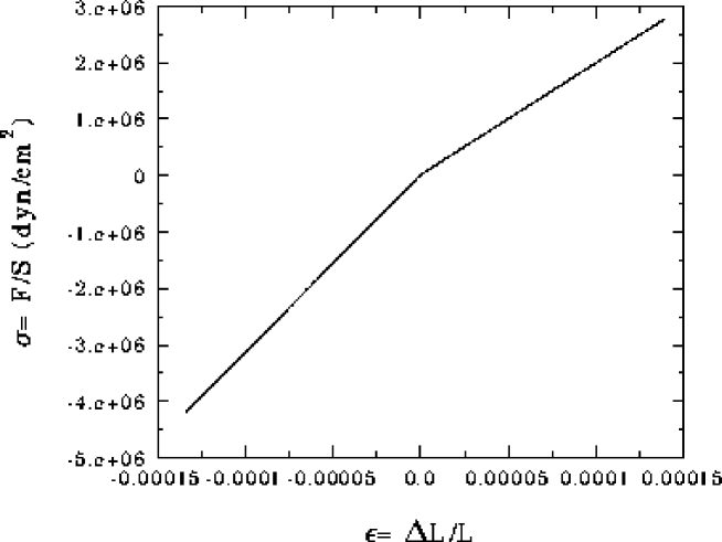
Figure 3: Typical result of a measurement of the effective Young modulus $K$, the horizontal stress $\sigma=F/S$ as a function of the vertical strain $\epsilon=\Delta L/L$. Positive and negative strain means elongation and compression of the solid, respectively. The values of $K$ were extracted from the slopes of the straight lines. One can observe the asymmetry of elongation and compression.

Fig. 3 shows an example of the results of the measurement of the Young modulus, the horizontal stress $\sigma=F/S$ as a function of the vertical strain $\epsilon=\Delta L/L$. The values of $K$ were extracted from the slope of the straight lines. It can be seen that elongation and compression of the system are not symmetric. The solid is more stiff under compression. The reason of the asymmetry is that in the case of elongation practically only the beams act but under compression one measures the common effect of the beams and the overlap force giving rise to a larger effective Young modulus.

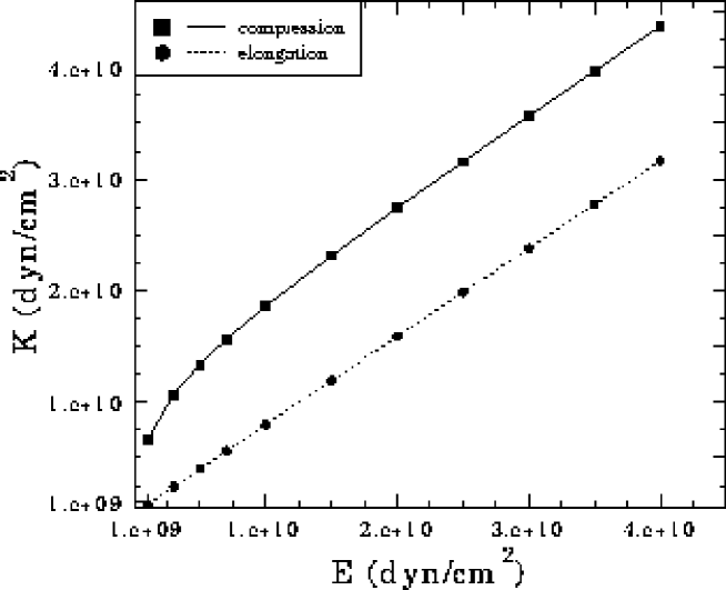
Figure 4: The effective (macroscopic) Young modulus $K$ of the granular solid measured under compression and elongation varying the beam Young modulus $E$ between $10^{9}dyn/cm^{2}$ and $4\cdot 10^{10}dyn/cm^{2}$. The grain bulk Young modulus was fixed to be $Y=10^{10}dyn/cm^{2}$.

Calculations were performed for elongation and compression of the sample fixing the value of the grain bulk Young modulus $Y$ and varying the beam Young modulus $E$. The results for $K$ are shown in Fig. 4. In the case of elongation $K$ is a linear function of $E$ as expected. For large $E$ the elongation and compression curves are parallel. The difference between them is determined by the grain bulk Young modulus $Y$ and by the geometry of the Voronoi tessellation. Small values of $E$ compared to $Y$ means that the cohesive force in the solid is small with respect to the repulsive overlap force. Under compression the polygons can move perpendicular to the loading in the direction of the free boundaries in the limiting case of small cohesion. Because of the dense packing (the initial packing fraction is one) the deformation tends to increase the overall volume resulting in dilatancy [20]. This effect gives rise to a small effective Young modulus, such that $K$ is even smaller than the grain bulk Young modulus $Y$.

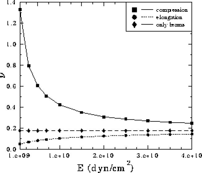
Figure 5: The Poisson ratio of the granular solid measured under compression and elongation. The values of $E$ and $Y$ are the same as in Fig. 4. The curve of the pure beam lattice was obtained by switching off the overlap force between the polygons.

For the Poisson ratio $\nu$ a similar asymmetry of elongation and compression is observed as shown in Fig. 5. The values of $\nu$ for elongation are smaller than for compression but for large $E$ both values approach the Poisson ratio of the pure beam lattice. In the limiting case of small cohesion $\nu$ can even exceed unity, due to the dilatancy mentioned above.

3.2 Explosion of a disc - shaped solid

The catastrophic fragmentation of solids will be studied in two different experimental situations: through an explosion which takes place inside the solid and through the impact with a projectile (stroke with a hammer). This chapter is devoted to study the explosion.

In the explosion experiment the detonation takes place in the center of a solid disc. The granular solid with disc - like shape was obtained starting from the Voronoi tessellation of a square and cutting out a circular disc in the center, see Fig. 2.

In the center of the solid we choose one polygon, which plays the role of the explosive. Initial velocities are given to the neighboring polygons perpendicular to their common sides with the central one. The sum of the initial linear momenta has to be zero, reflecting the spherical symmetry of the explosion. From these two constraints it follows that for a polygon having mass $m$ and a common boundary of length $S$ with the explosive center, the initial velocity is proportional to $\frac{S}{m}$. The sum of the initial kinetic energies defines the energy $E_{o}$ of the explosion. (For the parameter values and the initial conditions of the simulation see Table 1.)

As a result of these initial conditions a circularly symmetric outgoing compression wave is generated in the solid. In our context this means that there is a well - defined shell where the average longitudinal strain of the beams $<\epsilon>=<\Delta l/l>$ is negative. This compression wave is not homogeneous in the sense that not all the beams in this region are compressed . If the angle of a beam with respect to the radial direction is close to $\pi/2$ a beam can be slightly elongated within the compression wave.

Since the overall shape of the solid has the same symmetry as the compression wave it is possible to avoid geometrical asymmetries, which would arise for example in the explosion of a rectangular sample due to the corners. In the disordered solid the initial compression wave gives rise to a complicated stress distribution, in which the over-stressed beams break according to the breaking rule Eq. (9). The simulation is stopped if there is no beam breaking during 300 successive time steps. Free boundary conditions were used in all simulations.

Due to the beam breaking the solid eventually breaks apart, i.e. at the end of the process it consists of well separated groups of polygons. These groups of polygons, connected by the remaining beams, are the fragments. In the simulation of the explosion we are mainly interested in the time evolution of the fragmentation process and the mass distribution of fragments at the end of the process as a function of the breaking parameters.

All the calculations were performed on the CM5 of the CNCPST in Paris. We used the farming method, i.e. the same program runs on a variety of nodes with different initial setups. In our case 32 nodes were used with different seeds for the Voronoi generator, i.e. with differently shaped Voronoi cells.

3.2.1 The time evolution of the explosion

We performed two sets of calculations one allowing the beam breaking solely under elongation and another under elongation and compression, keeping all the other parameters of the simulation fixed. The evolution of the explosion and the resulting breaking scenarios are different in these two cases.

We can distinguish two regimes in the time evolution of the explosion: The initial regime is controlled by the compression wave and the disorder of the solid. The amplitude of the shock wave is proportional to the ratio of the average initial velocity of the polygons to the longitudinal sound speed of the solid. The width and the speed of the wave are mainly determined by the grain size and the Young moduli.

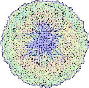
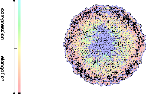
Figure 6: Explosion of a disc - shaped solid when only the stretched beams $(\epsilon>0)$ are allowed to break. Snapshots of the evolving system are presented when the initial compression wave reaches the boundary of the solid ($t=0.0001s$), the constructive interference of the incoming and outgoing elongation waves breaks the boundary layer ($t=0.001s$) and the final breaking scenario ($t=0.004s$). The color scale shows the color code for the beams. Black indicates that the strain is close to the stretching threshold $t_{\epsilon}$.

If the beams are not allowed to break under compression the compression wave can go outward almost unperturbed and an elongation wave is formed behind it. The elongated beams break according to the breaking rule Eq. (9) only for $\epsilon>0$. Due to the elongation wave a highly damaged region is created in the vicinity of the explosive center where practically all the beams are broken and all the fragments are single grains. This highly damaged region is called the mirror spot. Since the breaking of the beams, i.e. the formation of cracks in the solid, dissipates energy after some time the growth of the damage stops. The size of this mirror spot is determined by the initial energy of the explosion, by the dissipation rate and by the breaking thresholds (see Fig. 6).

During and after the formation of the mirror spot when the outgoing compression and elongation waves go through the solid the weakest (i.e. the longest and thinnest) beams break in an uncorrelated fashion creating isolated cracks in the system. The uncorrelated beam breaking is dominated by the quenched disorder of the solid structure. This first uncorrelated regime of the explosion process lasts till the compression wave reaches the free boundary of the solid.

From the free boundary the compression wave is reflected back with opposite phase generating an incoming elongation wave. The constructive interference of the incoming and outgoing elongation waves gives rise to a highly stretched zone close to the boundary. The beams having small angle with respect to the radial direction have the largest elongation. In this zone a large number of beams break causing usually the complete break-off of a boundary layer along the surface of the solid. The thickness of this detached layer is roughly half the width of the incoming elongation wave (see Fig.6). The fragments of this boundary layer fly away in the radial direction with a high velocity carrying with them a large portion of the total energy in the form of their kinetic energy. After that the system starts to expand. This overall expansion initiates cracks going from inside to outside and from outside to inside. The branching of single cracks and the interaction of different cracks give rise to the final fragmentation of the solid (Fig.6). This second part of the evolution of the explosion process is dominated by the correlation of the cracks.

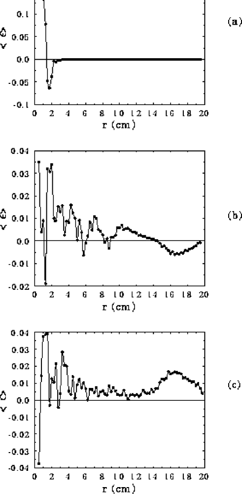
Figure 7: Propagation of the elastic wave in the disc - shaped solid. $(a)$ after $t=10^{-5}sec$ of the initial hit, $(b)$ after $t=3\cdot 10^{-4}sec$ the compression wave is approaching the boundary and $(c)$ after $t=5\cdot 10^{-4}$ the constructive interference of the incoming and the outgoing elongation waves.

The propagation of the elastic waves when the beam breaking is switched off is presented in Fig. 7. One can observe the peak of the initially imposed shock, the propagation of the compression and elongation waves and the formation of the highly stretched zones at the boundary.

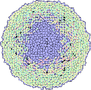
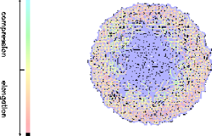
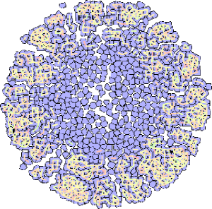
Figure 8: Explosion of a disc - shaped solid allowing the beam breaking under compression and elongation. The snapshots are taken at the same times as in Fig.6.

If the beams are allowed to break also under compression the time evolution of the process is significantly different. In the vicinity of the explosion center the initial compression wave governs the formation of the mirror spot. Where the compression wave passes all the beams break as long as the amplitude of the compression wave is larger than the threshold strain of the breaking criterion Eq. (9). Thus when the energy dissipation stops the growth of the damage the amplitude of the remaining compression wave is weaker and the size of the mirror spot is larger than it was in the previous case (Fig. 8). A significant part of the initial energy of the explosion is dissipated by the beam breaking and is transfered to the kinetic energy of the single polygons. So, less fragmentation can occur in the outer regions of the disc as compared to the case where breaking only occurs under elongation.

The compression wave reflects back from the free boundary but the constructive interference does not cause substantial damage along the surface (Fig.8). That is why the final breaking picture is different from the previous case.

3.2.2 The fragment mass distribution

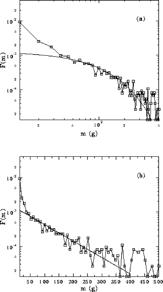
Figure 9: Fragment mass histogram allowing the beam breaking under compression and elongation. The breaking thresholds were chosen $t_{\epsilon}=3\%$ and $t_{\Theta}=4^{o}$. (a) shows on a logarithmic plot that $F(m)$ does not exhibit power law behavior and an exponential function seems to be a reasonable fit (bold line). (b) demonstrates the quality of the fit on a semi – logarithmic plot.

Fig. 6 and Fig. 8 show that the final breaking scenarios for the two breaking criteria are significantly different. When the beams are also allowed to break under compression there are only a few small fragments (apart from the single polygons) and a few much larger ones. This results in a fast decay of the fragment size distribution. The resulting fragment mass histogram is presented in Fig. 9. $F(m)$ denotes the number of fragments with mass $m$ divided by the total number of fragments. As can be seen from the logarithmic plot in Fig. 9 a, an exponentially decaying function can be a reasonable fit to these results for approximately one order of magnitude in mass. The quality of the fit is demonstrated in Fig. 9 b using a semi-logarithmic plot.

The application of Eq. (9) for $\epsilon>0$ only, is physically more relevant. In the following we present results of the mass distribution of the fragments as a function of the breaking parameters allowing the beam breaking solely under stretching. Changing $t_{\epsilon}$ and $t_{\Theta}$ in the breaking criterion Eq. (9) one can vary the relative contribution of the stretching and bending breaking modes, which can affect the crack formation and the final breaking scenario. The question is whether the mass distribution of the fragments is invariant under a change of $t_{\epsilon}$ and $t_{\Theta}$.

We performed simulations alternatively fixing $t_{\epsilon}$ and $t_{\Theta}$ and changing the value of the other one, keeping all the other parameters of the simulations fixed. In both cases the fraction of broken beams $p$ was monitored as a function of $s/l$, where $s$ and $l$ are the cross section and the length of a beam, respectively:

$$p(s/l)=b\frac{N_{broken}(s/l)}{N(s/l)},$$ (10)

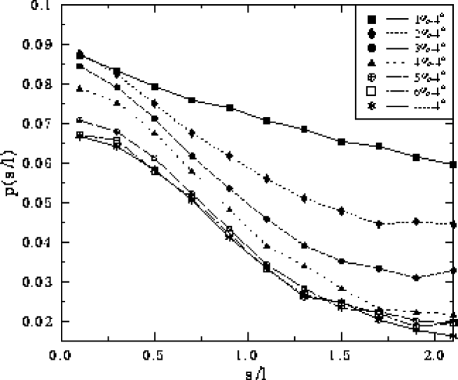
Figure 10: The fraction of broken beams as a function of $s/l$ varying the stretching threshold $t_{\epsilon}=1\%-6\%$. The fixed value of the bending threshold is $t_{\Theta}=4^{o}$. For increasing $t_{\epsilon}$ the curves tend to a limit, which coincides with the result obtained by switching off the stretching mode.

where $N(s/l)$ and $N_{broken}(s/l)$ denote the number of beams in the sample and the number of broken beams having a ratio of $s/l$. $b$ is a normalization constant. Fig. 10 and Fig. 11 show the results for fixed $t_{\Theta}=4^{o}$ varying the threshold strain $t_{\epsilon}$ from $1\%$ up to $6\%$ and for fixed $t_{\epsilon}=3\%$ varying the threshold angle $t_{\Theta}$ from $1^{o}$ up to $7^{o}$, respectively. The curves are normalized in such a way that their integrals are equal to the overall fraction of broken beams $p_{o}$, i.e. $\int p(s/l)d(s/l)=p_{o}$. Here $p_{o}=N_{broken}/N$, where $N$ and $N_{broken}$ denote the total number of beams in the sample and the total number of broken beams, respectively. One can observe that $p(s/l)$ is a monotonically decreasing function for all parameter values, which shows that longer and thinner beams are always easier to break, as expected. In Fig. 10 for small $t_{\epsilon}$ and in Fig. 11 for small $t_{\Theta}$ the solid is more fragile, so it undergoes strong damage. This results in a larger $p_{o}$ and a rather flat breaking fraction $p(s/l)$. The curves belonging to increasing $t_{\epsilon}$ and $t_{\Theta}$ lie below each other. Since by increasing a breaking threshold, the contribution of the corresponding breaking mode becomes less important, the fixed mode starts to dominate the breaking and determines the limiting curve. The results obtained by switching completely off one of the breaking modes confirm this argument.

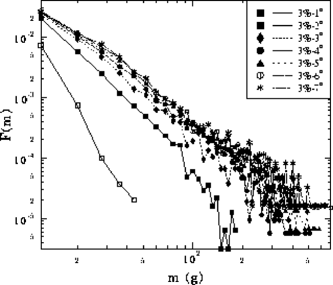
Figure 13: The fragment mass histograms varying the bending threshold $t_{\Theta}=1^{o}-7^{o}$. The stretching threshold is fixed $t_{\epsilon}=3\%$. The contribution of the single polygons are ignored. For increasing $t_{\Theta}$ the curves tend to a limit, which is determined by the fixed stretching mode.

The fragment mass histograms are presented in Fig 12 and Fig. 13. The lower cutoff of the histograms is determined by the size of the unbreakable polygons (smallest fragments) while the upper cutoff is given by the finite size of the system (largest fragment). Larger values of the overall breaking fraction $p_{o}$ entails that the system is broken into smaller pieces.

The histograms follow a power law for practically all the parameter pairs for at least one order of magnitude in mass, such that we seem to have

$$\vspace{0.4cm}F(m)\sim\alpha m^{-\beta}.\vspace{0.4cm}$$ (11)

The effective exponents $\beta$ were obtained from the estimated slopes of the curves. The results are presented in Table 2. Apart from the case of extremely small breaking parameters the exponent $\beta$ only slightly varies around $\beta=2.0$, indicating a more or less universal behavior within the accuracy, with which $\beta$ was determined ($\pm 0.05$). Fig. 14 shows that increasing $t_{\epsilon}$ and $t_{\Theta}$ a crossover appears in $F(m)$, i.e. there are two exponents. As we have mentioned, the initial compression wave gives rise to the break-off of a boundary layer, the thickness of which is determined by the wavelength and by the breaking parameters. For larger $t_{\epsilon}$ and $t_{\Theta}$, when the system is tougher, a detachment of the fragmentation of the boundary layer and the bulk of the solid appears. The boundary gives the main contribution to the small fragments (containing $\sim$ 2 – 6 polygons) and the fragmentation of the bulk dominates the range of the larger ones. In these cases the exponents $\beta$ in Table 2 were obtained in the limit of large fragments.

3.3 Impact of a projectile

Besides the explosion a catastrophic fragmentation of solids can also be generated by an impact with a projectile. In nature one of the most spectacular examples is that the size distribution of meteorites and asteroids shows power law behavior. These objects are believed to have originated from the fracture of primitive planets due to collisions [1, 4].

We applied our model to study the fragmentation of a rectangular solid block (e.g. a block of concrete) due to an impact allowing the beam breaking solely under stretching $\epsilon>0$. One polygon at the lower middle part of the block is given a high velocity directed inside the block simulating an elastic collision with a projectile. The boundary conditions and the stopping condition were the same as in the explosion experiment. The breaking thresholds were chosen $t_{\epsilon}=3\%$ and $t_{\Theta}=4^{o}$.

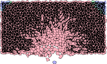
Figure 15: Fragmentation of a concrete block composed of elastic grains. One grain at the lower middle part of the block is given a high velocity directed inside the block. Here the velocity was $400m/s$. The size of the block was chosen to be $40cm\times 20cm$. Snapshots of the evolving system are presented at $t=0.0004s$, $t=0.0015s$ and $t=0.003s$.

The evolution of the fragmenting solid block is presented in Fig. 15. As in the case of the explosion, the initially generated compression wave plays a significant role. Since the energy of the collision is concentrated around the impact site of the projectile the damage is the largest in that region. The completely destroyed zone, where all the beams are broken stretches inside the solid in the forward direction resulting in the break-up of the solid. When the shock wave reaches the boundary at the side of the solid opposite to the collision point it gives rise to the break-off of a boundary layer. The fragments of this layer fly away in the forward direction with a high velocity. Some small fragments from the vicinity of the collision point are scattered backward. The damage in the direction perpendicular to the projectile is not strong, the broken boundary layer is thicker and the speed of the fragments is smaller.

Results of laboratory experiments on high velocity impacts can be found in Refs. 3,4. In Ref. 4 a picture series obtained by a high speed camera is presented showing the time evolution of an impact experiment. Our results are qualitatively in good agreement with the experimental observations.

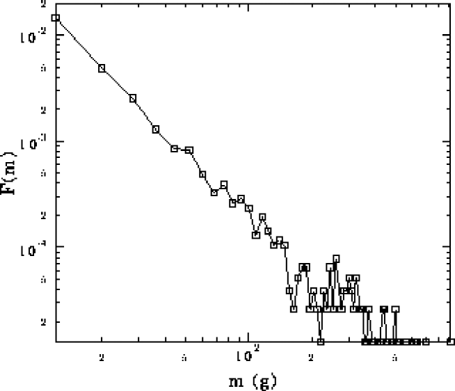
Figure 16: Fragment mass histogram of the collision experiment. The size of the solid block was chosen to be $40cm\times 20cm$ and the initial impact velocity given to a grain in the lower middle part was $400m/s$.

The resulting fragment mass histogram $F(m)$ is presented in Fig. 16. Similarly to the explosion experiment, $F(m)$ shows power law behavior for approximately one order of magnitude in mass. The value of the effective exponent is $\beta=1.98\pm 0.05$.

4 Conclusion

We have studied shock fragmentation in two dimensions using a cell model similar to the one introduced by Potapov et al [12, 13]. We found a qualitative difference in the breaking process when breaking occurs under traction or under both, traction and compression. If only traction force can produce cracks a power-law distribution of the fragment sizes is evidenced with a rather universal exponent around two in good agreement with most experimental observations. Interesting is the effect of lamination in which a surface layer half the width of the elastic wave is detached and ejected with high velocity. This effect has been observed experimentally in high speed impacts.

With the present study we have evidenced that the full treatment of elasticity and wave propagation are necessary if one wants to reproduce subtleties of fragmentation as lamination or the dependence on compressive breaking. Still our study makes a certain number of technical simplifications which might be important for a full quantitative grasp of fragmentation phenomena. Most important seems to us the restriction to two dimensions, which should be overcome in future investigations. The existence of elementary, non-breakable polygons restricts fragmentation on lower scales and hinders us from observing the formation of powder of a shattering transition [10].

An advantage of our model with respect to most other fragmentation models is that we can follow the trajectory of each fragment, which is often of big practical importance and that we know how much energy each fragment carries away. The polygonal structure of our solid allows us to realistically model granular or polycrystalline matter, and considering as well cell repulsion as beam connectivity gives us a rich spectrum of possibilities ranging from breaking through bending to the effect of dilatancy. If one or the other mechanism is turned off we have the extreme cases of an elastic homogeneous solid and a compact dry granular packing.

Figure 2: Elastic beams connecting the Voronoi polygons in a disc - shaped sample. Because of the randomness in the Voronoi tessellation one has also a random lattice of beams.

Figure 11: The fraction of broken beams as a function of $s/l$ varying the bending threshold $t_{\Theta}=1^{o}-7^{o}$. The fixed value of the stretching threshold is $t_{\epsilon}=3\%$. For increasing $t_{\Theta}$ the curves tend to a limit, which coincides with the result obtained by switching off the bending mode.

Figure 12: The fragment mass histograms varying the stretching threshold $t_{\epsilon}=1\%-6\%$. The bending threshold is fixed $t_{\Theta}=4^{o}$. The contribution of the single polygons are ignored. For increasing $t_{\epsilon}$ the curves tend to a limit, which is determined by the fixed bending mode.

Figure 14: The fragment mass histogram for $t_{\epsilon}=6\%$ and $t_{\Theta}=4^{o}.$ One can observe a crossover between two fragmentation regimes.

$Parameter$	$Symbol$	$Unit$	$Value$
Density	$\rho$	$g/cm^{3}$	5
Grain bulk Young modulus	$Y$	$dyn/cm^{2}$	$10^{10}$
Beam Young modulus	$E$	$dyn/cm^{2}$	$5\cdot 10^{9}$
Time step	$dt$	$s$	$10^{-6}$
Diameter of the solid	$d$	$cm$	$40$
Average # of polygons	$n$		$1100$
Energy of the explosion	$E_{o}$	$erg$	$5\cdot 10^{9}$
Average initial speed	$v_{o}$	$m/s$	$200$
Estimated sound speed	$c$	$m/s$	$900$

Table 1: The parameter values used in the simulations.

$t_{\Theta}=4^{o}$		$t_{\epsilon}=3\%$
$t_{\epsilon}$	$\beta$	$t_{\Theta}$	$\beta$
1 $\%$	(4.34)	$1^{o}$	$(4.42)^{\mathit{a}}$
2 $\%$	2.39	$2^{o}$	2.5
3 $\%$	2.01	$3^{o}$	1.98
4 $\%$	1.97	$4^{o}$	2.01
5 $\%$	1.95	$5^{o}$	1.96
6 $\%$	1.96	$6^{o}$	1.95
		$7^{o}$	1.97

Table 2: The values of the exponent $\beta$ for different breaking thresholds.

References

- [1] D. L. Turcotte, J. of Geophys. Res. Vol. 91 B2, 1921 (1986).
- [2] N. Arbiter, C. C. Harris and G. A. Stamboltzis, Soc. of Min. Eng. 244, 119 (1969).
- [3] T. Matsui, T. Waza, K. Kani and S. Suzuki, J. of Geophys. Res. 87 B13, 10968 (1982).
- [4] A. Fujiwara and A. Tsukamoto, Icarus 44, 142 (1980).
- [5] M. Matsushita and T. Ishii, Fragmentation of long thin glass rods, Department of Physics, Chuo University (1992).
- [6] L. Oddershede, P. Dimon, and J. Bohr, Phys. Rev. Lett. 71, 3107 (1993).
- [7] M. Matsushita and K. Sumida, How do thin glass rods break? (Stochastic models for one - dimensional fracture), Chuo University, Vol. 31, pp. 69-79 (1981).
- [8] S. Steacy and C. Sammis, An automaton for fractal patterns of fragmentation, Nature 353 250 (1991).
- [9] G. Hernandez, H. J. Herrmann, Physica A 215, 420 (1995).
- [10] S. Redner, in: Statistical Models for the Fracture of Disordered Media (North Holland, Amsterdam, 1990).
- [11] H. Inaoka, H. Takayasu, preprint.
- [12] A. V. Potapov, M. A. Hopkins and C. S. Campbell, Int. J. of Mod. Phys. C 6, 371 (1995).
- [13] A. V. Potapov, M. A. Hopkins and C. S. Campbell, Int. J. of Mod. Phys. C 6, 399 (1995).
- [14] H. J. Herrmann, in: 3rd Granada Lectures in Computational Physics, eds. P. L. Garrido and J. Marro (Springer, Heidelberg, 1995)
- [15] H. J. Tillemans, H. J. Herrmann, Physica A 217, 261 (1995).
- [16] K. B. Lauritsen, H. Puhl and H. J. Tillemans, Int. J. of Mod. Phys. C 5, 909 (1994).
- [17] H. J. Herrmann and S. Roux (eds.) Statistical Models for the Fracture of Disordered Media (North Holland, Amsterdam, 1990).
- [18] H. J. Herrmann, A. Hansen, S. Roux, Phys. Rev. B 39, 637 (1989).
- [19] S. Roux, in Ref. 17.
- [20] Y. M. Bashir and J. D. Goddard, J. Rheol. 35, 849 (1991).