Entropy derivation for cluster methods in non-Bravais lattices

I INTRODUCTION

The cluster-variation method (CVM) is considered as a generalization of the traditional mean-field (Bragg-Wiliams[1]) theory taking only one-point configurations into account. The first-neighbor pair correlations were handled in the method developed by Bethe for square lattice [2]. The accuracy of this technique were improved by Kramers and Wannier, who chose a square cluster on which the probabilities of each configuration were taken into consideration [3]. The variational method was generalized by Kikuchi for different lattice structure using a large class of clusters [4]. The above authors used combinatorial methods to determine the entropy as a function of cluster configuration probabilities. Since then the CVM has been reformulated by several authors. These formulations were motivated by the cumbersome calculations when determining ensemble configurations for large clusters in three-dimensional lattices. Barker showed the equivalence between a generalization of quasi-chemical approximation and CVM [5]. Hijmans and De Boer developed a systematic scheme for obtaining the free energy expressed by cluster variables [6]. Woodbury found that many of the previous results were reproducible in a direct manner using the composition law of information theory [7]. Introducing a generalized cumulant expansion of the entropy the CVM was reformulated by Morita [8]. This latter formulation is strongly related to the Möbius inversion [9, 10, 11]. A systematic counting and classification of clusters were carried out by Gratias et al. [12] for general crystal structures including some non-Bravais lattices. Sanchez et al. developed a general formalism based on the description of configurational cluster functions in terms of an orthogonal basis in the multidimensional space of site variables [13]. Several authors investigated the convergence of CVM when using larger and larger clusters [9, 14, 15, 16, 17].

Recently the CVM is widely used to determine phase diagrams in different systems (for reviews see the works by de Fontaine [18, 19] and further references therein). In the present work we suggest a simple way for the entropy derivation which is not related to the Gibbs formalism and may be used for dynamical (non-equilibrium) systems too. Furthermore this method is applicable to non-Bravais lattices which are very important for practice (e.g. superionic conductors, metal-hydrogen systems, intercalation alloys, etc). For this purpose the CVM is reformulated by showing how to construct the probability of a given particle (spin) configuration as a product of cluster configuration probabilities taking the translation symmetries and self-consistency into account. These conditions can be satisfied by using different approximations equivalent to those mentioned above. Now we concentrate on the entropy per elementary cells which is related to the conditional entropy introduced in information theory [20]. As a result the entropy as well as the energy are expressed as a function of the probabilities of cluster configurations. Thus we have a free energy to be minimized with respect to these variables for obtaining thermodynamic equation of states.

In the subsequent section the essence of this method is illustrated on the one-dimensional lattice. This idea is adapted for the two-dimensional system in Sec. III. Here, a graphical representation of the construction of configuration probabilities will be introduced. This technique is used to obtain entropy expressions for two non-Bravais lattices formed by the interstitial sites in body-centered- and face-centered-cubic lattices in Secs. IV and V. Finally the results are summarized in Sec. VI.

II One-dimensional lattice

In the one-dimensional model a site variable $\eta_{i}$ ($i=1,...,N$) denotes the state of the $i$th lattice point. In the lattice-gas formalism ($\eta_{i}=0$ or 1), however, the subsequent formulae remain valid for those systems characterized by $Q$ states at each site (e.g. $\eta_{i}=0$, $1$, $Q-1$). The function $f_{N}=f(\eta_{1},...,\eta_{N})$ describes the probability of a configuration specified by the $\eta_{i}$ variables. Similarly, we introduce a cluster of $k$ subsequent sites on which the probability of a configuration is defined by $p_{k}(\eta_{1},\ldots,\eta_{k})$. If the system is translation invariant, then

$$\sum_{\eta_{i}\atop i<j,\;i>j+k-1}f_{N}=p_{k}(\eta_{j},\eta_{j+1},\ldots,\eta_{j+k-1})$$ (1)

for arbitrary $1\leq j\leq N-k$. Consequently, the set of $p_{k}(\eta_{1},\ldots,\eta_{k})$ functions satisfies the following relations:

$$p_{k}(\eta_{1},\ldots,\eta_{k}) = \sum_{\eta_{0}}p_{k+1}(\eta_{0},\eta_{1},\ldots,\eta_{k})\ ,$$ (2)

$$p_{k}(\eta_{1},\ldots,\eta_{k}) = \sum_{\eta_{k+1}}p_{k+1}(\eta_{1},\ldots,\eta_{k},\eta_{k+1})\ ,$$ (3)

for $k>1$ and

$$\sum_{\eta_{1}}p_{1}(\eta_{1})=1\ .$$ (4)

The probabilities of the $k$-point configurations are completely described by introducing $2^{k-1}$ parameters [21]. More precisely, the number of independent variables may be less than $2^{k-1}$ when additional symmetries (e.g. reflection, particle-hole) are taken into consideration.

In $n$-point approximation the probability of a particle configuration is expressed as:

$$f_{N}=p_{n}(\eta_{1},\ldots,\eta_{n})\prod_{i=n+1}^{N}P_{1}(\eta_{i}|\eta_{i-n+1},\ldots,\eta_{i-1})$$ (5)

where

$$P_{1}(\eta_{i}|\eta_{i-n+1},\ldots,\eta_{i})={p_{n}(\eta_{i-n+1},\ldots,\eta_{i})\over p_{n-1}(\eta_{i-n+1},\ldots,\eta_{i-1})}$$ (6)

describes the conditional probability of finding $\eta_{i}$ state at the $i$th site ($n<i\leq N$) if the cluster configuration in the previous $n-1$ points is given. The above expression is self-consistent in the sense that it satisfies the condition of translation invariance [see Eq. (1)] for $k\leq n$. To check it the summation should be performed with respect to the first and/or last site variables step by step using the expressions (2) and (3).

Choosing the Boltzmann constant to be unit the entropy is

$$S=-\sum_{\{\eta_{i}\}}f_{N}\ln f_{N}\ ,$$ (7)

where the summation runs over all the possible configurations. Substituting Eq. (5) into (7) one obtains that

$$S= - \sum_{\{\eta_{i}\}}f_{N}\ln p_{n}(\eta_{1},\ldots,\eta_{n})$$ (8)

$$- \sum_{\{\eta_{i}\}}f_{N}\sum_{i=n+1}^{N}\ln P_{1}(\eta_{i}|\eta_{i-n+1},\ldots,\eta_{i-1})\ .$$ (9)

According to Eq. (1) this expression may be simplified and in the thermodynamic limit the entropy per lattice sites is

$$s = \lim_{N\to\infty}{S\over N}$$ (10)

$$= -\sum_{\eta_{1},\ldots,\eta_{n}}p_{n}(\eta_{1},\ldots,\eta_{n})\ln\left({p_{n}(\eta_{1},\ldots,\eta_{n})\over p_{n-1}(\eta_{1},\ldots,\eta_{n-1})}\right)\ .$$ (11)

As shown by Woodbury [7] this quantity is equivalent to the conditional entropy introduced in information theory [20]. According to Eqs. (2) and (3) the above entropy may be written in the following form:

$$s={\cal S}_{n}-{\cal S}_{n-1}$$ (12)

where

$${\cal S}_{n}=-\sum_{\eta_{1},\ldots,\eta_{n}}p_{n}(\eta_{1},\ldots,\eta_{n})\ln{p_{n}(\eta_{1},\ldots,\eta_{n})}\;.$$ (13)

These expressions are very convenient for the CVM.

Using the techniques mentioned in the Introduction the entropy of the one-dimensional system was previously derived by several authors [2, 4, 7]. Here it is worth mentioning that the pair ($n=2$) approximation reproduces the exact solution for the one-dimensional Ising model with nearest-neighbor interaction.

The present derivation is based on the fact that the configuration probability given as product of conditional probabilities is self-consistent, i.e. it satisfies the Eq. (1). The generalization of this approach for higher dimensions is not trivial, approximations are required as it will be shown in the following section.

III Square lattice

In order to explore the difficulties arising on a square lattice we consider first the probability of a configuration constructed on the analogy of the one-dimensional system using square cluster configuration probabilities. In a translation invariant system we introduce the function $p_{4}(\eta_{a},\eta_{b},\eta_{c},\eta_{d})$ (clockwise labelling) characteristic to the probability of any four-point configurations on sites $a,b,c$ and $d$ forming a square with nearest neighbor bond sides. From these quantities the three-, two- and one-point configuration probabilities (on the corresponding subclusters) can be derived on the analogy of Eqs. (2) and (3). Henceforth we restrict ourselves to systems having fourfold symmetry. In this case the three- and two point configuration probabilities are independent of the cluster orientation.

The system with $L\times M$ sites can be covered by $(L-1)\times(M-1)$ overlapping squares. Following this covering procedure the $f_{N}$ function is built up from $p_{4}(\eta_{a},\eta_{b},\eta_{c},\eta_{d})$ functions. To visualize this calculation a graphical representation of this product is introduced as displayed in the subsequent figures. Here the squares, triangles, solid lines and closed circles represent $p_{4}$, $p_{3}$, $p_{2}$ and $p_{1}$ functions in the numerator with site variable arguments corresponding to the positions. If these quantities appear in the denominator then the above symbols will be plotted by dashed lines or open circles. The size of the closed (or opened) circles refer to the exponents of $p_{1}$ functions which may differ from 1 (or -1) in the examples investigated.

FIG. 1.: Graphical representation of an intermediate stage when constructing configuration probability as a product in four-point approximation. Squares and closed circles represent four-point and one-point cluster configuration probabilities in the numerator with arguments corresponding to their position. Dashed lines denote two-point configuration probabilities in the denominator.

According to a direct (naive) way the addition of the site variable $\eta_{a}$ to the product as shown in Fig. 1 is performed via the following conditional probability:

$$P_{1}(\eta_{a}|\eta_{b},\eta_{c},\eta_{d})={p_{4}(\eta_{a},\eta_{b},\eta_{c},\eta_{d})\over p_{3}(\eta_{b},\eta_{c},\eta_{d})}\;.$$ (14)

Unfortunately, this construction results in a configuration probability $f_{N}$ which is not self-consistent. This difficulty may be circumvented if all the $p_{3}$ functions appearing in the expressions are approximated as

$$p_{3}(\eta_{b},\eta_{c},\eta_{d}) = \sum_{\eta_{a}}p_{4}(\eta_{a},\eta_{b},\eta_{c},\eta_{d})$$ (15)

$$= {p_{2}(\eta_{b},\eta_{c})p_{2}(\eta_{c},\eta_{d})\over p_{1}(\eta_{c})}\;.$$ (16)

This situation is illustrated graphically in Fig. 1. Within the framework of this approximation the self-consistency of the resultant $f_{N}$ is easily checked because the summation defined in Eq. (16) can be executed graphically too. As a result the square transforms into an ”angle” built up from two $p_{2}$ and a $p_{1}$ functions. For example, the summation over $\eta_{a}$ in Fig. 1 removes the $abcd$ square as well as the touched dashed lines and bullet. This procedure may be repeated for all the $\eta_{i}$ variables belonging to “free” site of a square until only the desired square remains on the screen. As a consequence the entropy per sites may be evaluated on the analogy of the one-dimensional calculation. Neglecting boundary effects in the thermodynamic limit it obeys the following form:

$$s={\cal S}_{4}-2{\cal S}_{2}+{\cal S}_{1}$$ (17)

where the ${\cal S}_{n}$ quantities are defined on the analogy of Eq. (13) and the symmetries mentioned above are taken into consideration. This formula is equivalent to those derived by Kramers and Wannier [3].

The three-point (“angle”) approximation suggested by Kikuchi [4] can also be reproduced by the present approach. In this case the lattice is covered with triangles as shown in Fig. 2.

FIG. 2.: In three-point approximation the configuration probabilities are built up as a product of $p_{3}$ functions (triangles) divided by $p_{1}^{\nu}$ terms where the value of $\nu=1,2$ is denoted by the size of open circles.

The condition of self-consistency is fulfilled if the two-point configuration probabilities are approximated in the mathematical manipulations as

$$p_{2}^{\prime}(\eta_{b},\eta_{c}) = \sum_{\eta_{a}}p_{3}(\eta_{a},\eta_{b},\eta_{c})=p_{1}(\eta_{b})p_{1}(\eta_{c})\;,$$ (18)

$$p_{2}(\eta_{a},\eta_{c}) = \sum_{\eta_{b}}p_{3}(\eta_{a},\eta_{b},\eta_{c})=p_{1}(\eta_{a})p_{1}(\eta_{c})\;$$ (19)

where we used the notation indicated in Fig. 2 and similar formula is assumed for $p_{2}(\eta_{a},\eta_{b})$. On the basis of Fig. 2 we can construct $f_{N}$ and the entropy per lattice sites is

$$s={\cal S}_{3}-2{\cal S}_{1}$$ (20)

Notice that in this approximation $f_{N}$ does not reflects the fourfold symmetry assumed in the system in comparison with those represented graphically in Fig. 1. This approximation takes into account all the pair correlation via $p_{3}$, however, only a quarter of the possible three-point correlations is handled.

The reproduction of pair approximation is worth mentioning for later convenience. One can image that in the above three-point approximation the $p_{3}$ function is constructed from $p_{2}$ functions as

$$p_{3}(\eta_{a},\eta_{b},\eta_{c})={p_{2}(\eta_{a},\eta_{b})p_{2}(\eta_{c},\eta_{a})\over p_{1}(\eta_{a})}\;.$$ (21)

To satisfy the condition of self-consistency one has to use the following approximation:

$$\sum_{\eta_{a}}{p_{2}(\eta_{a},\eta_{b})p_{2}(\eta_{c},\eta_{a})\over p_{1}(\eta_{a})}=p_{1}(\eta_{b})p_{1}(\eta_{c})\;.$$ (22)

The graphical representation of the product construction is illustrated in Fig. 3. The entropy obtained agrees with the result derived by Bethe [2].

FIG. 3.: Graphical representation of configuration probability in pair approximation. Solid lines represent two-point configuration probabilities in the numerator. The sizes of open circles refer to the exponents (1, 2 or 3) of $p_{1}$ functions in the denominator.

We can choose larger clusters to increase the accuracy of CVM. The above covering technique is required to have a translation invariant $f_{N}$ constructed as a product of conditional probabilities. The main problem is how to construct the denominator of the conditional probability characteristic to the probability of configurations on the overlapping region. In general the following rule of thumb seems to be useful for finding the approximations required to satisfy the condition of self-consistency. The configuration probability on the overlapping region should be constructed from the largest subclusters of the present clusters. This idea works well for $k\times k$-point clusters. The graphical representation becomes confused if one chooses large non-compact clusters. At the same time, the numerical solution is also very complicate for large clusters.

The generalization of the present approach to other (two- or three-dimensional) Bravais lattices is straightforward. As the simplest example for a non-Bravais lattice one can study the chess-board like sublattice (antiferromagnetic) ordering on the square lattice. In this situation the lattice is divided into two ($A$ and $B$) interpenetrating sublattices with different average occupations (or magnetizations). This system can be described by introducing two types of four-point configuration probabilities, namely $p_{4}^{A}(\eta_{a},\eta_{b},\eta_{c},\eta_{d})$ and $p_{4}^{B}(\eta_{a},\eta_{b},\eta_{c},\eta_{d})$ where the upper indices denotes the sublattice to which site $a$ belongs. The entropy per sites is derived by repeating the above calculation with using alternately $p_{4}^{A}$ and $p_{4}^{B}$ “squares” during the covering. The result is similar to those given by Eq. (17), namely

$$s={1\over 2}\sum_{\alpha}\left[{\cal S}^{\alpha}_{4}-2{\cal S}^{\alpha}_{2}+{\cal S}^{\alpha}_{1}\right]$$ (23)

where $\alpha=A,B$ and fourfold symmetry is assumed.

IV Tetrahedral sites in BCC lattice

In the BCC lattice the interstitial atoms are positioned at the tetrahedral sites exhibiting a non-Bravais lattice. These sites can be divided into six (equivalent) sublattices labelled by $\alpha=1,\ldots,6$ (see Fig. 4).

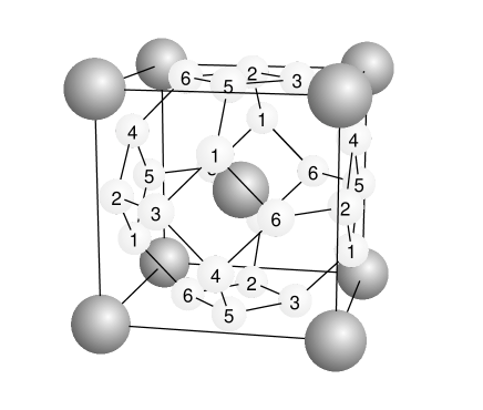
FIG. 4.: Sublattice structure of tetrahedral interstitial sites (small spheres) in BCC lattice (large spheres).

In the six-sublattice mean-field approximation the configuration probability is defined as a product of the corresponding one-point configuration probabilities $p_{1}^{\alpha}(\eta_{i})$. This approximation is evidently self-consistent and results in the following entropy (henceforth normalized by the number of host lattice points):

$$s=\sum_{\alpha}{\cal S}^{\alpha}_{1}\;.$$ (24)

This approximation is used previously to demonstrate the possibility of two subsequent phase transitions during the ordering process in AgI [22]. This method considers all the phases conserving translation symmetry of the host lattice. The cubic symmetry of these states is broken when the sublattice occupations are different.

In order to have a more accurate description of these states we have to distinguish three different four-point clusters positioned on the faces of a cubic cell. The probabilities of the configurations in these clusters are denoted by $p_{4}^{\beta}(\eta_{a},\eta_{b},\eta_{c},\eta_{d})$ where $\beta=x,y,z$ refers to the face on which the square is positioned. When the particle configuration is built up cube by cube as a product of conditional probabilities then we add 12 new site variables to the system. We choose these variables to be located on the three connecting faces (see Fig. 5). The connections toward the touched cubes are taken into account by the squares standing out the cubic cell plotted in Fig. 5. In fact, these 18-point clusters are used for covering. Now, however, the probability of the configurations on these clusters are constructed from $p_{4}^{\beta}$ and $p_{1}^{\alpha}$ functions as represented graphically in the figure.

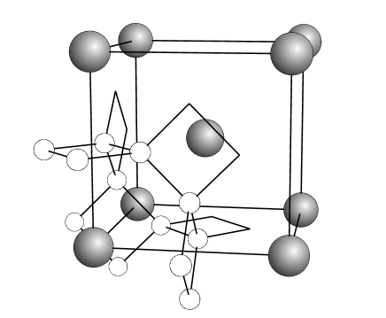
FIG. 5.: Graphical representation of the conditional probability when adding a cubic cell to the system. Squares and open circles denote $p_{4}^{\beta}$ and $p_{1}^{\alpha}$ functions in the numerator and denominator.

The open circles at the corners of the outstanding squares denote that the configuration probability on the overlapping region is approximated by a product of $p_{1}^{\alpha}$ functions in accordance with the rule of thumb mentioned above. The $f_{N}$ function obtained is self-consistent if a product $p_{1}^{\alpha}p_{1}^{\alpha^{\prime}}$ is substituted for the two-point configuration probabilities appearing during the summation process, for example:

$$\sum_{\eta_{c},\eta_{d}}p_{4}^{\beta}(\eta_{a},\eta_{b},\eta_{c},\eta_{d})=p_{1}^{\alpha}(\eta_{a})p_{1}^{\alpha^{\prime}}(\eta_{b})$$ (25)

where $\alpha$ and $\alpha^{\prime}$ refers to the corresponding sublattices. After some algebraic manipulation the entropy is given as:

$$s=\sum_{\beta}{\cal S}^{\beta}_{4}-\sum_{\alpha}{\cal S}^{\alpha}_{1}\;.$$ (26)

One can choose different ways of covering for obtaining the same result. For example, first the $(x,y,0)$ sites are covered by distinct horizontally oriented squares ($p_{4}^{z}$), then we add all the vertical squares ($p_{4}^{x}$ and $p_{4}^{y}$) to the system having two sites in the $(x,y,1/4)$ plane, and so on.

Instead of suggesting other approximations for this lattice structure, in the subsequent section we demonstrate how the present method can be used for such a lattice exhibiting two types of interstitial sites.

V Interstitial sites in FCC lattice

In the FCC lattice there are one octahedral and two tetrahedral interstitial sites per lattice points as illustrated in Fig. 6. These sites can be divided into three (FCC) sublattices. The three-sublattice formalism allows us to study a rich variety of states conserving the translation invariance of the host lattice.

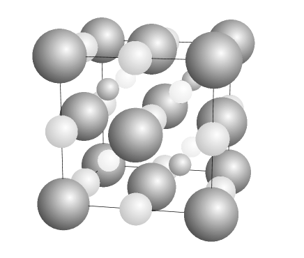
FIG. 6.: The three-sublattice structure of tetrahedral (small spheres with two gray scales) and octahedral (middle spheres) interstitial sites in FCC lattice (large dark spheres).

Notice that in this non-Bravais lattice the octahedral sites are positioned at every second centers of the cubes appearing in NaCl-type structure of the tetrahedral sites. This feature inspires the choice of simple cubic and body-centered-cubic clusters (see Fig. 7) for the construction of $f_{N}$.

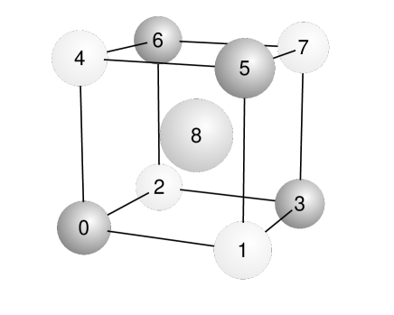
FIG. 7.: Cubic (nine-point) cluster on interstitial sites in FCC lattice. The figures on the spheres represent site indices.

The condition of self-consistency is fulfilled if we use the following approximations during summations:

$$\sum_{\eta_{7},\eta_{8}}p_{9}(\eta_{0},\ldots,\eta_{8})=\sum_{\eta_{7}}p_{8}(\eta_{0},\ldots,\eta_{7})=$$ (27)

$${p_{4}(\eta_{0},\eta_{1},\eta_{4},\eta_{5})p_{4}(\eta_{0},\eta_{1},\eta_{2},\eta_{3})p_{4}(\eta_{0},\eta_{2},\eta_{4},\eta_{6})p_{1}(\eta_{0})\over p_{2}(\eta_{0},\eta_{1})p_{2}(\eta_{0},\eta_{2})p_{2}(\eta_{0},\eta_{4})}$$ (28)

and similar expressions are assumed when instead of $\eta_{7}$ the sum runs over $\eta_{i}$ where $i\leq 6$. Here the site indices of the arguments of $p_{8}$ agree with those shown in Fig. 7 excepting 8. The same formulae will appear in the denominators of the corresponding conditional probabilities. Consequently, the entropy is

$$s={\cal S}_{9}+{\cal S}_{8}-6{\cal S}_{4}+6{\cal S}^{(T1-T2)}_{2}-{\cal S}^{(T1)}_{1}-{\cal S}^{(T2)}_{1}$$ (29)

where the upper indices in the ${\cal S}_{n}$ functions indicate sublattices to which the cluster sites belong if it is necessery. In this expression the cubic symmetry is taken into consideration.

Despite the symmetries of the above cubic clusters the number of parameters will be large leading to difficulties in the numerical calculations. The number of parameters is drastically reduced if the cubic clusters (as well as the whole system) are built up from smaller ones. In the simplest case we can introduce a triangle cluster formed by “nearest-neighbor” sites belonging to different sublattices (e.g. sites 0, 1 and 8 in Fig. 7). Suppose that $p_{3}(\eta_{a},\eta_{b},\eta_{c})$ denotes the probabilities of configurations on these clusters independently of its orientation, where $\eta_{a}$, $\eta_{b}$ and $\eta_{c}$ belong to the octahedral and tetrahedral sublattices, respectively. This choice is very convenient because we have only seven parameters for the variation technique. The configuration probabilities on the nine-point cluster shown in Fig. 7 is expressed by these quantities in such a way that the edges will be represented with equal weight, that is

$$p_{9}(\eta_{0},\ldots,\eta_{8}) = {p_{3}(\eta_{8},\eta_{0},\eta_{1})p_{3}(\eta_{8},\eta_{3},\eta_{1})p_{3}(\eta_{8},\eta_{5},\eta_{1})\over p_{2}^{2}(\eta_{8},\eta_{2})}$$ (30)

$$\times {p_{3}(\eta_{8},\eta_{3},\eta_{7})p_{3}(\eta_{8},\eta_{3},\eta_{2})p_{3}(\eta_{8},\eta_{6},\eta_{4})\over\tilde{p}_{2}^{2}(\eta_{8},\eta_{1})p_{1}(\eta_{8})}$$ (31)

where $p_{2}$ and $\tilde{p}_{2}$ are distinguished because their second arguments belong to different tetrahedral sublattices. The whole system may be covered by these body-centered-cubic clusters overlapping each other at single tetrahedral sites. In this approximation the entropy is given as

$$s= 6 {\cal S}_{3}-2{\cal S}^{(O-T1)}_{2}-2{\cal S}^{(O-T2)}_{2}$$ (32)

$$- {\cal S}^{(O)}_{1}-3{\cal S}^{(T1)}_{1}-3{\cal S}^{(T2)}_{1}$$ (33)

This triangle approximation, however, is not definite. Another result may be obtained on the basis of Bethe’s method as follows. The elementary cell of this non-Bravais lattice has three sites chosen to form a triangle cluster defined above (see triangle $abc$ in Fig. 8).

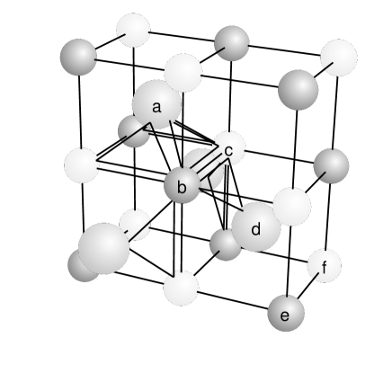
FIG. 8.: Positions of $p_{3}$ functions connecting the triangle $abc$ to its nearest neighbors having the same orientation in case of triangle-triangle pair approximation.

Now this triangle is considered as a single site variable with $2^{3}$ possible values and the triangle-triangle pair correlations are handled on the analogy of pair approximation. For example, the configuration probability on the triangle pair $abc$–$def$ is defined as a $p_{3}p_{3}p_{3}/(p_{2}p_{1})$ product. Due to the FCC symmetries each triangle has twelve nearest neighbors. In this case, only those triangle-triangle pairs are considered which are connected to each other through a single triangle cluster as illustrated in Fig. 8. As a result the entropy obeys the following form:

$$s= 6 {\cal S}_{3}-2{\cal S}^{(O-T1)}_{2}-2{\cal S}^{(O-T2)}_{2}-{\cal S}^{(T1-T2)}_{2}$$ (34)

$$- {\cal S}^{(0)}_{1}-2{\cal S}^{(T1)}_{1}-2{\cal S}^{(T2)}_{1}$$ (35)

which reproduces Eq. (33) if $p_{1}(\eta_{b})p_{1}(\eta_{c})$ is substituted for $\hat{p}_{2}(\eta_{b},\eta_{c})$. Evidently, the approximations required by the self-consistency are different in these situations. The latter formula is used to check the mean- field phase diagrams of a lattice-gas model suggested to describe the ordering processes in alkali-fullerides [23]. The systematic comparison of the possible approximations goes beyond the scope of the present work.

VI Conclusions

The derivation of entropy for cluster techniques is reformulated by showing how to construct the configuration probabilities as a product of conditional probabilities when building up the system from overlapping clusters. In one-dimensional system this product is obviously self-consistent. For higher dimensional systems, however, some approximations are required to fulfill the self-consistency which is relevant when expressing the entropy per sites as a conditional entropy introduced in information theory.

A graphical representation of the product is suggested to make the calculations treatable. Using this technique we have reproduced some traditional results derived on square lattices. Due to its simplicity, this approach is easily applicable to complicated lattices. Using this method entropy expressions are derived on two non-Bravais lattices, formed by the interstitial sites of BCC and FCC structures, which may be useful for the investigation of many real systems.

In fact, the present derivation of entropy is equivalent to combinatorial calculations. However, it provides a better understanding of the approximations applied. It is emphasized that these methods assume merely translation invariance despite some other techniques based on the formalism of equilibrium statistical physics. As a consequence the entropy expressions remain valid for those non-equilibrium systems whose stationary states satisfy this condition.

REFERENCES

- [1] W. L. Bragg and E. J. Williams, Proc. Roy. Soc. (London) A 145, 699 (1934).
- [2] H. A. Bethe, Proc. Roy. Soc. (London) A150, 552 (1935).
- [3] H. A Kramers and G. H. Wannier, Phys. Rev. 60, 252 (1941).
- [4] R. Kikuchi, Phys. Rev. 81, 988 (1951).
- [5] J. A. Barker, Proc. Roy. Soc. (London) A216, 45 (1953).
- [6] J. Hijmans and J. De Boer, Physica 21, 471, 485, 499 (1955).
- [7] G. W. Woodbury, J. Chem. Phys. 47, 270 (1967).
- [8] T. Morita, J. Phys. Soc. Jpn. 12, 753 (1957); J. Math. Phys. 13, 115 (1972).
- [9] A. G. Schlijper, Phys. Rev. B 27, 6841 (1983).
- [10] G. An, J. Stat. Phys. 52, 727 (1988).
- [11] T. Morita, J. Stat. Phys. 59, 819 (1990).
- [12] D. Gratias, J. M. Sanchez, and D. de Fontaine, Physica 113, 315 (1982).
- [13] J. M. Sanchez, F. Ducastle, and D. Gratias, Physica A 128, 334 (1984).
- [14] M. Kurata, R. Kikuchi, and T. Watari, J. Chem. Phys. 21, 434 (1953).
- [15] R. Kikuchi and S. G. Brush, J. Chem. Phys. 47, 195 (1967).
- [16] A. G. Schlijper, J. Stat. Phys. 35, 285 (1984).
- [17] A. Pelizzola, Phys. Rev. E 49, R2305 (1994).
- [18] D. de Fontaine, in Solid State Physics, Vol. 47, edited by H. Ehrenreich and D. Turnbull (Academic London, 1994) p. 33.
- [19] D. de Fontaine, in Alloy Phase Stability, Vol. 163 of NATO ASI Series E Applied Sciences, Edited by G. M. Stocks and A. Gonis (Kluwer Academic Publishers, Dordrecht 1989).
- [20] C. E. Shannon and W. Weaver, The Mathematical Theory of Communication (The University of Illinois Press, Urbana, 1949).
- [21] H. A. Gutowitz, J. D. Victor, and B. W. Knight, Physica 28D, 18 (1987).
- [22] G. Szabó, J. Phys. C 19, 3775 (1986).
- [23] L. Udvardi and G. Szabó, E-print: cond-mat/9512001