Critical Properties of Random Quantum Potts and Clock Models

Abstract

We study zero temperature phase transitions in two classes of random quantum systems -the $q$-state quantum Potts and clock models. For models with purely ferromagnetic interactions in one dimension, we show that for strong randomness there is a second order transition with critical properties that can be determined exactly by use of an RG procedure. Somewhat surprisingly, the critical behaviour is completely independent of $q$ (for $2\leq q<\infty$). For the $q>4$ clock model, we suggest the existence of a novel multicritical point at intermediate randomness. We also consider the $T=0$ transition from a paramagnet to a spin glass in an infinite range model. Assuming that the transition is second order, we solve for the critical behaviour and find $q$ independent exponents.

The effects of randomness on the properties of quantum many-body systems have been the subject of experimental and theoretical studies for many years[1]. Despite this, understanding of phenomena where quantum effects, randomness, and interactions are all important is rather poor, and there are as yet few reliable theoretical techniques. Recent work [2, 3, 4, 5] has focussed attention on simple quantum statistical mechanical systems with randomness as a useful starting point to obtain insights into such phenomena, and some progress has been made. In this paper we study analytically the effects of disorder on the properties of two classes of quantum models with discrete symmetry. These are to be regarded as quantum versions of the classical $q$-state Potts and the $q$-state clock models [6]. Studies of the corresponding classical models have yielded a fair amount of insight into the competing effects of randomness, interactions, and thermal fluctuations[7]. For instance, classical Potts spin glasses have been studied extensively as a paradigm for understanding the properties of orientational glasses[7].

We first consider the zero temperature quantum phase transition in random (purely ferromagnetic) $1$-dimensional quantum Potts and clock chains. For the $1$-d random transverse field Ising model (RTFIM), which (as we shall see below) is the $q=2$ case of these models, a wealth of essentially exact information has recently been obtained in a remarkable paper[2] by Fisher using a real space renormalization group procedure. Here we show that this procedure can similarly be used to obtain exact critical properties of strongly random $q$-state Potts and clock chains for all $q$, and implies, remarkably, that there is no $q$ dependance in any of the exponents or the scaling functions. This is in stark contrast to the pure problem where the properties of the transition depend crucially on the value of $q$[6, 8]. In addition, considerations on the effects of weak randomness suggest the possibility that for any amount of randomness, the Potts model for any $q$ and the clock model for $2\leq q\leq 4$ are described by the strong randomness fixed point. For the clock chain with $q>4$, we suggest the existence of a multicritical point at a finite strength of randomness. Next we consider the zero temperature transition from a paramagnet to a spin glass in infinite-ranged quantum Potts and clock models. Again building on work on the $q=2$ case[5, 4], and assuming a second order transition, we find that the critical properties are independent of $q$.

The models are defined in terms of a variable that can assume $q$ possible states (which we denote $|0\rangle~{},|1\rangle~{},\cdots,|q-1\rangle$) on the sites of a $d$-dimensional lattice. The classical Potts (clock) interaction in the presence of a uniform external “magnetic” field $H$ along the ‘$0$’ direction is

$${\cal H}_{P,int} = -\sum_{\langle i,j\rangle}J_{ij}\delta_{n_{i}n_{j}}-2H\sum_{i}(\delta_{n_{i},0}-\frac{1}{q})~{}~{}~{}~{}~{}~{}~{}~{}~{}~{}~{}~{}~{}~{}~{}~{}~{}~{}~{}~{}~{}~{}~{}(Potts)$$ (1)

$${\cal H}_{C,int} = -\sum_{\langle i,j\rangle}2J_{ij}\cos(\frac{2\pi}{q}(n_{i}-n_{j}))-2H\sum_{i}\cos\frac{2\pi n_{i}}{q}~{}~{}~{}~{}~{}~{}~{}(Clock)$$ (2)

We introduce quantum fluctuations into these models by adding at each site a “transverse field” term that attempts to change the state of the variable at that site. Thus we consider the quantum Hamiltonians

$${\cal H}_{P} = -\sum_{i}h_{i}\left(\sum_{n_{i},n^{\prime}_{i}=0}^{q-1}\frac{1}{q}|n_{i}\rangle\langle n^{\prime}_{i}|\right)+{\cal H}_{P,int}~{}~{}~{}~{}~{}~{}~{}~{}~{}~{}~{}~{}~{}~{}~{}~{}~{}~{}~{}~{}~{}~{}~{}(Potts)$$ (3)

$${\cal H}_{C} = -\left(\sum_{n_{i}=0}^{q-1}h_{i}(|n_{i}\rangle\langle n_{i}+1|+h.c)\right)+{\cal H}_{C,int}~{}~{}~{}~{}~{}~{}~{}~{}~{}~{}~{}~{}~{}~{}~{}~{}~{}~{}(Clock)$$ (4)

(We identify $|n_{i}+q\rangle=|n_{i}\rangle$). Through out the paper we will assume that the ${h_{i}}$ and ${J_{ij}}$ are independent random variables drawn from some distributions $P_{1}(h)$ and $P_{2}(J)$ respectively. Note that at $H=0$, the Hamiltonian ${\cal H}_{P}$ is invariant under a global permutation $|n\rangle\rightarrow|n^{\prime}\rangle$ of the states at each site. For ${\cal H}_{C}$, the symmetry is a global cyclic rotation $|n\rangle\rightarrow|n+1\rangle$. Clearly for $q=2$, both these models reduce to the transverse field Ising model. For general $q$, just as in the Ising case, the “transverse field” term plays the role of a kinetic energy that opposes the tendency to order due to the interaction term. Also as in the Ising case, the $d$-dimensional $q$-state quantum Potts (clock) model Eqn. 3 (4) at zero temperature may be regarded as the transfer matrix in the $\tau$-continuum limit of a $d+1$-dimensional $q$-state classical Potts (clock) model[9] with disorder constant along one direction.

In the absence of disorder, the mapping to the classical $d+1$-dimensional pure problem provides a rather complete picture of the possible phases and the transitions between them. For instance (at zero $H$), the ferromagnetic (i.e $J>0,~{}~{}h>0$) quantum Potts chain has a first order transition for $q>4$, and a second order transition for $q\leq 4$ (for which all the exponents are known exactly and depend on the value of $q$)[6, 10]. The ferromagnetic clock chains, on the other hand, have, for $q>4$, a quasi-long-range ordered (QLRO) phase sandwiched between a truely long-range ordered phase and a disordered phase[8] . For $q\leq 4$, the quasi-long-range ordered phase disappears and is replaced by an ordinary second order phase transition for which again all the exponents are known exactly[6, 8]. Below we will see that randomness drastically modifies this picture.

We start with $1$-d chains in which all the $h_{i}$’s and $J_{ij}$’s are random but positive and $H=0$. Defining the total magnetization as $M=\sum_{i}\langle s_{i}\rangle$ with $s_{i}=\delta_{n_{i},0}-\frac{1}{q}$ for the Potts model and $s_{i}=\cos\frac{2\pi n_{i}}{q}$ for the clock model, it is clear that as the overall relative strength of the $h_{i}$’s is decreased, there will be a transition from a phase with $M=0$ to one with $M\neq 0$. We assume that the randomness is strong and follow closely a real-space RG procedure used by Fisher[2] to extract an enormous amount of information on the RTFIM ($q=2$ case). The basic idea behind this procedure[11] is to successively eliminate the strongest coupling $\Omega=max\{h_{i},J_{i,i+1}\}$ in the chain and get an effective Hamiltonian for the low energy degrees of freedom. First consider the case when the maximum coupling is a field, say $h_{i}$. We eliminate the site $i$, and obtain, using second order perturbation theory, a new effective bond between the sites $i-1$ and $i+1$ of strength $J=(J_{i-1,i}J_{i,i+1})/\kappa h_{i}$ where $\kappa$ is $q/2$ for the Potts model and $(1-\cos(\frac{2\pi}{q}))/(1+\delta_{q,2})$ for the clock model. On the other hand, if the maximum coupling is a bond $J_{i,i+1}$, we replace the sites $i$ and $i+1$ by a single Potts (or clock) degree of freedom with an effective field $h=(h_{i}h_{i+1})/\kappa J_{i,i+1}$ where $\kappa$ is the same as before (as may be expected from a duality which these models can be shown to possess[12]). The $q$ dependance is only through $\kappa$. As in Ref.[2], we convert these recursion relations into flow equations for the distributions $P_{1}(\zeta=\ln(\Omega/J),\Gamma=\ln(\Omega_{I}/\Omega))$ and $P_{2}(\beta=\ln(\Omega/h),\Gamma=\ln(\Omega_{I}/\Omega))$ where $\Omega_{I}$ is the initial value of the maximum coupling and find

$$\frac{\partial P_{1}}{\partial\Gamma}= \frac{\partial P_{1}}{\partial\zeta}+P_{1}(P_{1}(0,\Gamma)-P_{2}(0,\Gamma))+$$ (6)

$$~{}~{}~{}~{}~{}~{}+~{}~{}P_{2}(0,\Gamma)\int d\zeta_{1}d\zeta_{2}P_{1}(\zeta_{1},\Gamma)P_{1}(\zeta_{2},\Gamma)\delta(\zeta-\zeta_{1}-\zeta_{2}-\ln\kappa)$$

and similarly with $P_{1}\leftrightarrow P_{2}$ (as expected from duality). When now we rescale and look for critical fixed points, the value of $\ln\kappa$ becomes irrelevant at low energies (so long as it is finite). The resulting probability distributions in the scaling limit described by the fixed point are independent of $q$. In general it is necessary to keep track of two joint distributions - that of bond lengths and bond strengths at scale $\Gamma$ and that of cluster lengths, their magnetic moments and “transverse” field strengths at scale $\Gamma$. Both these distributions will be independent of $q$ in the scaling limit. Thus the value of $q$ merely determines a high-energy cutoff $E_{c}\sim\Omega_{I}e^{-|\ln\kappa|}$ (below which one should be in order to observe scaling behaviour) but does not affect the scaling behaviour itself. Note that since this cutoff goes to zero as $q\rightarrow\infty$, our results hold only for finite $q$.

At this point it is tempting to conclude that all the Potts and clock chains will have identical critical properties. However we note that, in general, identical probability distributions do not necessarily imply identical physical properties. For instance, the pure problems trivially have identical distributions but have very different properties. However, as shown by Fisher[2], the distributions of the logarithmic couplings $\zeta$ and $\beta$ become infinitely broad asymptotically at low energies. It is then straightforward to see that due to this extreme broadness all physical quantities (such as magnetization or mean correlation function) are described by $q$-independent scaling functions and exponents. The only $q$-dependence occurs in some non-universal constants. We illustrate this point with the example of the scaling of the magnetization $M(H,\delta)$ as a function of small external applied field $H(>0)$ and a dimensionless measure $\delta$ of the deviation from criticality[13]. In the presence of a magnetic field $H$, the energy levels of an otherwise-free cluster of magnetic moment $\mu$ split into a ground state $|n=0\rangle$ and other excited states with a gap $E_{H}=2\mu qH$ for the Potts case and (atleast) $E_{H}=2\mu H(1-\cos\frac{2\pi}{q})$ for the clock case. Proceeding exactly as for the RTFIM, we stop the RG when the maximum coupling $\Omega\sim E_{H}$. Due to the extreme broadness of the distribution, an asymptotically exact expression for $M(H,\delta)$ is obtained by aligning all the remaining clusters in the direction of the magnetic field. Thus

$$M(H,\delta) = \bar{\mu}\times({\rm total~{}~{}number~{}~{}of~{}~{}active~{}~{}({\em i.e}~{}~{}undecimated)~{}~{}spins~{}~{}at~{}~{}scale~{}~{}}\Gamma_{H}=\ln\frac{D_{H}}{H})~{}~{}~{}$$

$$+~{}~{}{\rm corrections}$$

where $\bar{\mu}$ and $D_{H}$ are non-universal and possibly $q$ dependent constants. The key point now is that the number of active spins at a given scale $\Gamma$ is entirely a property of the joint distribution of cluster lengths, magnetic moments, and field strengths which is $q$-independent in the scaling limit. Consequently, the universal scaling function describing $M(H,\delta)$ will be the same for all $q$. The $q$ dependence is only in the non-universal quantities $\bar{\mu}$ and $D_{H}$. Through similar reasoning, one can establish that the mean correlation function $\bar{C}(x)=\overline{\langle s_{0}s_{x}\rangle}$ is also described by a $q$-independent scaling function.

Thus the Potts and clock chains for any $q$ (with strong ferromagnetic randomness) do indeed have critical properties identical to those of the RTFIM (the $q=2$ case) for which detailed results are available[2]. We point out some salient features below. The spontaneous magnetization vanishes at the transition with exponent $\beta=\frac{3-\sqrt{5}}{2}$. The mean and typical correlation functions at the critial point decay as $\bar{C}(x)\sim\frac{1}{|x|^{\beta}}$ and $-\ln C_{typ}(x)\sim\sqrt{|}x|$ respectively for large $|x|$. In the disordered side, there are $2$ correlation lengths, characterizing the decay of mean and typical correlations, which diverge with exponents $\nu=2$ and $\tilde{\nu}=1$ respectively. The magnetization scaling function is known exactly, and the scaling function for the mean correlation function known up to the solution of a linear ordinary differential equation. Asymptotically at the critical point “lengths” scale as the square of the logarithm of “energies” (unlike most other quantum transitions where lengths scale as a power of the energies). On either side of the transition there are Griffiths regions. In the Griffiths region of the disordered phase, the order-parameter susceptibility diverges as $T\rightarrow 0$ as a power with an exponent weaker than Curie. Throughout this region, the magnetization increases as a power (with logarithmic corrections) of an applied external magnetic field with a continuously varying exponent. Similarly in the Griffiths region of the ordered side the stiffness vanishes for an infinite system, and the susceptibility diverges as $T\rightarrow 0$ as a power with an exponent that is stronger than Curie. Very far from the critical point, there are of course the more conventional strongly ordered and disordered phases.

The RG procedure used above is valid only if the randomness in the initial distributions $P_{1}$ and $P_{2}$ is strong. Clearly it cannot address the question whether, if the initial distribution is narrow, the low energy properties will still be described by the strong randomness fixed point found above. Some insights on this matter are provided by considering the effect of weak randomness on the pure systems. So long as the pure transition is second order, weak randomness is relevant at the fixed point if $\nu<2/d$ (the generalized Harris criterion[14]) where $d$ is the spatial dimension. From the known values of $\nu$[6, 10] for $q\leq 4$ for the Potts and clock chains, we conclude that weak randomness is indeed relevant. The simplest scenario then is that for $q\leq 4$, the RG flows take the system to the strong randomness fixed point for any amount of randomness in the initial distributions. The situation however is different for $q>4$. We discuss the Potts and clock cases separately. The pure Potts chain for $q>4$ has a first order transition. For first order phase transitions in classical systems, it has been argued that any amount of “bond” randomness converts the transition to second order[15] for $d\leq 2$. Extension of this argument to quantum systems would then suggest that the random $q>4$ quantum Potts chain has a second order transition for any amount of randomness. We conjecture that this transition is described by the strong randomness fixed point.

We now turn to the clock model for $q>4$ where there is an intermediate quasi-long-range ordered phase separating a truely ordered phase from the paramagnetic phase. The phase transitions into the QLRO phase from either side are of the Kosterlitz-Thouless type with $\nu=\infty$, therefore implying by the Harris criterion that weak randomness is irrelevant. The QLRO phase is described by a line of fixed points. A straightforward perturbative calculation shows that weak randomness is irrelevant along this entire line[16]. Thus weak disorder does not change the nature of the phase diagram in this case while for strong disorder, as we have seen earlier, there is a single second order phase transition (surrounded by Griffiths regions) and no QLRO phase. Understanding how the phase diagram changes as the strength of the disorder increases is an interesting open question. We speculate that as the strength of the disorder is increased, the two lines of Kosterlitz-Thouless transitions bounding the QLRO phase merge at a multicritical point. Beyond this point the QLRO phase disappears, and there is a single second order transition described by the strong randomness fixed point (See Figure 1). We do not however have any strong arguments ruling out more complicated scenarios (such as for instance, a new intermediate phase separating the QLRO phase from the region with a single second order transition).

Having described the $1$-dimensional random ferromagnetic systems in some detail, it is natural to ask if there are other non-trivial yet solvable cases. One such example is provided by infinite-range spin glass models. As is well-known, classical SG models display a complicated and rich structure even for infinite-range interactions. There has been some recent progress in understanding the zero temperature quantum phase transition into a spin glass phase in the transverse field Ising model (the $q=2$ case of our models)[5, 4]. The basic idea is quite straightforward[17]. One first performs the disorder average using the replica trick and reduces the problem to an effective single site problem with a self-consistency condition on the auto-correlation function. At the critical point it is possible to solve the self-consistency condition by making a suitable ansatz for the long-time behaviour of the auto-correlation function. For the Ising case, one finds that the critical auto-correlation decays as $1/\tau^{2}$ at large imaginary time $\tau$[5, 4]. In addition, in the paramagnetic side, there is an energy gap that vanishes on approaching the transition with an exponent $1/2$ with logarithmic corrections. Repeating the analysis for the $q$-state quantum Potts or clock spin glass model, and assuming a second order transition, we find[16] that the critical exponents once again remain the same as the Ising case. However the assumption of a second order transition may be questionable (atleast for the Potts and odd-$q$ clock models) since the finite temperature phase transition from the paramagnetic side in the corresponding classical models is not of the conventional second order type[18].

In summary, we have shown that for strongly random ferromagnetic quantum $q$-state Potts and clock chains, the critical properties are completely independent of $q$ for $2\leq q<\infty$. This result is a priori surprising as in the pure models the possible phases and the transitions between them are known to depend crucially on the value of $q$. We have also studied the zero temperature transition from a paramagnet to a spin glass in these models with infinite range interactions. If the transition is second order, the critical exponents have $q$-independent values. We conclude by noting the following implications of our work and by raising some open questions. Our results imply that for classical $2$-d Potts and clock models with disorder correlated along one direction, the critical properties of the finite temperature phase transition are independent of the value of $q$. It is interesting that numerical simulations by Chen et. al.[19] on the classical $2$-d $8$-state Potts model with uncorrelated disorder find a second order transition with exponents equal to the classical $2$-d Ising values. This suggests the possibility that the $q$-independence found here with correlated disorder also holds with uncorrelated disorder. However an analytic calculation by expanding in $q-2$ [20] does find $q$-dependence in the exponents. Further studies to address this issue will be welcome. From our discussion of the phase diagram for the clock chains with $q>4$ (Figure 1), there arises the possibility of a novel multicritical point at finite randomness. Verification of the existence of this point, perhaps numerically, is an interesting open problem. Also interesting is the question of whether this $q$ independence persists in higher dimensional ferromagnetic models. For the spin glass models, one approach to go beyond our results, atleast in high enough dimensions, would be to study a Landau theory analogous to that developed for the Ising and rotor models[4]. Such a study may also resolve the issue of whether the transition is second order or not.

We thank Subir Sachdev, R.Shankar, N.Read, and D.S.Fisher for useful discussions and comments. This research was supported by NSF Grants No.  DMR-92-24290 and DMR-91-20525.

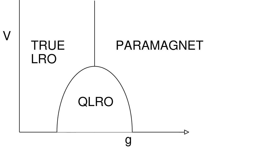
FIG. 1.: One possible (schematic) phase diagram for the $q>4$ random quantum clock chain. $g=\overline{\ln h}$ is a parameter that measures the strength of quantum fluctuations and $V$ is a measure of the strength of the randomness.

REFERENCES

- [1] An example is the metal-insulator transition. For a review, see P.A.Lee and T.V.Ramakrishnan, Rev. Mod. Phys. 57, 287 (1985). As another example see work on the dirty boson problem by M.P.A.Fisher , P.Weichmann, G.Grinstein, and D.S.Fisher, Phys. Rev. B40, 546 (1989)
- [2] D.S.Fisher,Phys. Rev. Lett. 69, 534 (1992); D.S.Fisher,Phys. Rev. B51, 6411 (1995).
- [3] R.Shankar and G.Murthy, Phys. Rev. B36, 536 (1987).
- [4] N.Read, S.Sachdev, and J.Ye, Phys. Rev. B52, 384 (1995); J.Ye, S.Sachdev, and N.Read, Phys. Rev. Lett. 70, 4011 (1993)
- [5] J.Miller and D.Huse, Phys. Rev. Lett. 70, 3147 (1993)
- [6] F.Y.Wu, Rev. Mod. Phys. 54, 235 (1982)
- [7] K.Binder and J.D.Reeger, Adv. in Physics, 41,547 (1992)
- [8] J.Jose, L.Kadanoff, S.Kirkpatrick, and D.R.Nelson, Phys. Rev. B16, 1217 (1977) ; S.Elitzur, R. Pearson, and J. Shigemitsu, Phys. Rev. D19, 3698 (1979)
- [9] J.Solyom and P.Pfeuty, Phys. Rev. B 24, 218 (1981); L.Turban, J. Phys. A 18, 2313 (1985)
- [10] M.P.M. den-Nijs, J. Phys. A12, 1857 (1979).
- [11] S.K.Ma, C.Dasgupta, and C.-k.Hu, Phys.Rev. Lett. 43, 1434 (1979); C.Dasgupta and S.K.Ma, Phys. rev. B22, 1305 (1980)
- [12] This is well-known for the pure -d quantum systems; see Ref [6]. In the presence of randomness, under the duality transformation, the distributions of and get interchanged.
- [13] In Ref[2] for the RTFIM, was related exactly to some properties of the original distributions. Such a relation does’nt seem possible here.
- [14] A.B.Harris, J. Phys. C 7, 1671 (1974); J.T.Chayes, L.Chayes, D.S.Fisher, and T.Spencer, Phys. Rev. Lett. 57, 2999 (1986).
- [15] K.Hui and A.N.Berker, Phys. Rev. Lett. 62, 2507 (1989)
- [16] T. Senthil and S.N. Majumdar, unpublished
- [17] A.J.Bray and M.A.Moore, J. Phys. C 13, L655 (1980)
- [18] D.J.Gross, I.Kanter, and H.Sompolinsky, Phys. Rev. Lett. 55, 304 (1985)
- [19] S.Chen, A.M.Ferrenberg, and D.P.Landau, Phys. Rev. Lett., 69, 1213 (1992)
- [20] A.W.W.Ludwig, Nucl. Phys. B330, 639 (1990)