CELLULAR AUTOMATA FOR TRAFFIC FLOW:
ANALYTICAL RESULTS

Abstract

We use analytical methods to investigate cellular automata for traffic flow. Two different mean-field approaches are presented, which we call site-oriented and car-oriented, respectively. The car-oriented mean-field theory yields the exact fundamental diagram for the model with maximum velocity $v_{max}=1$ whereas in the site-oriented approach one has to take into account correlations between nearest-neighbour sites. Going beyond mean-field using the so-called $n$-cluster approach our results for $v_{max}>1$ are in excellent agreement with numerical simulations. We also present a modified cellular automaton which is closely related to a two-dimensional dimer model.

1 Introduction

In 1992 Nagel and Schreckenberg [1] introduced a cellular automaton model describing traffic flow of $N$ cars on a single lane. In this model the street is divided into $L$ boxes (’cells’) of a certain length (for realistic applications 7.5 meters) which can be occupied by at most one car or be empty. The cars have an internal parameter (’velocity’) which can take on only integer values $v=0,1,2,\ldots,v_{max}$. The dynamics of the model is described by update rules for the velocities and the motion of the cars. The update rules are given by the following four steps [1]:
1) Acceleration: $v_{i}\rightarrow v^{\prime}_{i}=v_{i}+1$ (if $v_{i}<v_{max}$)
2) Slowing down: $v_{i}\rightarrow v^{\prime}_{i}=d_{i}-1$ (if $d_{i}\leq v_{i}$)
3) Randomization: $v^{\prime}_{i}\rightarrow v^{\prime\prime}_{i}=v^{\prime}_{i}-1$ (with probability $p$) for $v^{\prime}_{i}>0$
4) Car motion: Car moves $v^{\prime\prime}_{i}$ sites
Here $v_{i}$ is the velocity of car $i$ and $d_{i}$ is the distance between cars $i$ and $i+1$. Without step 3) the dynamics would be purely deterministic and the system shows strong dependence on the initial condition. The randomization takes into account natural fluctuations in the driver’s behaviour. All cars are updated simultaneously (parallel update) and we here use periodic boundary conditions (“Indianapolis situation”). For the analytical calculation it is usually advantagous to change the order of the steps into 2-3-4-1, since after step 1) there are no vehicles with velocity 0. This change in order than has to be taken into account in the calculation of the flux (fundamental diagram).

Most of the results for this cellular automaton have been obtained from simulations [2]. Basically there are two different methods to implement the rules [3]. In the car-oriented approach the state is characterized by the occupancy of each individual site (which might be empty or occupied by a car with velocity $0,1,\ldots,v_{max}$). In the car-oriented method on the other hand one has two lists, one with the velocities of the cars and one in which the distance to the next car ahead is stored. For small densities $c=N/L$ the last method is preferable in simulations and for higher densities the first one.

2 Site-Oriented Approach

In the site-oriented approach the state of the system is characterized by the probability $P_{n}(t)$ to find at time $t$ a site in the state $n$, where $n=0$ for an empty site and $n=1,2,\ldots,v_{max}$ for a site occupied by a car with velocity $n$ . Since in mean-field theory one neglects correlations between $n$ neighbouring sites one can write down iteration equations for the $P_{n}$ in the stationary state [3]. These equations then allow a calculation of the fundamental diagram. In Fig. 1 results for the “realistic” value [1] $v_{max}=5$ are compared with the simulations. The mean-field flow is much too small showing the importance of correlations.

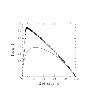
Figure 1: Fundamental diagram for $v_{max}=5$ and $p=1/2$. Shown are the results of the simulations and the mean-field theory.

The results of mean-field theory can be improved systematically by the so-called $n$-cluster approximation [4, 3]. The $n$-cluster method takes into account correlations between neighbouring sites and reduces to mean-field theory for $n=1$. In order to get a closed set of equations one uses conditional probabilities for the overlap of neighbouring clusters [4, 3]. Unfortunately, one then has to deal with a system of $(v_{max}+1)^{n}$ nonlinear equations which in general cannot be solved analytically.

Surprisingly, for $v_{max}=1$ the 2-cluster approximation already yields the exact result. The probabilities $P(\sigma_{1},\sigma_{2})$ to find a 2-cluster in a state $(\sigma_{1},\sigma_{2})$ (where – due to the ordering 2-3-4-1 – $\sigma_{j}=0$ denotes an empty site and $\sigma_{j}=1$ a site occupied by a car with velocity 1) are given by

$$P(1,0) = P(0,1)={1-\sqrt{1-4qc(1-c)}\over 2q},$$

$$P(0,0) = 1-c-P(1,0),\qquad P(1,1)=c-P(1,0),$$ (1)

where $c=N/L$ is the density of cars and $q=1-p$. The corresponding flow is just $f(c,p)=qP(1,0)$, i.e.

$$f(c,p)=\frac{1-\sqrt{1-4qc(1-c)}}{2}.$$ (2)

Note that – in contrast to what one finds using random-sequential dynamics – parallel dynamics yield the well-known “bunching” observed in real traffic, i.e. empty sites and cars attract each other ($P(0)P(1)=c(1-c)\leq P(1,0)$). This means that there exists an attraction between two cars separated by an empty site.

Figure 2: Fundamental diagram for $v_{max}=1$ and $p=1/2$. Shown are the results of the simulations and the 1- and 2-cluster approximations. The 2-cluster result is exact.

For higher velocities the $n$-cluster approximation does not become exact reflecting the fact that long-range correlations exist for $v_{max}>1$. In Fig. 3 we compare the results of the $n$-cluster approximation for $n=1,\ldots,5$ with simulations. The $n$-cluster results converge quite fast (the difference between the results for $n=4$ and $n=5$ is less than 1%) and already the $n=5$ result is in very good agreement with the simulations.

Figure 3: Fundamental diagram for $v_{max}=2$ and $p=1/2$. Shown are the results of the simulations and the $n$-cluster approximations for $n=1,2,\ldots 5$.

3 Car-Oriented Approach

In the car-oriented mean-field approach one introduces probabilities $D_{n}(t)$ for finding at time $t$ exactly $n$ empty sites in front of a vehicle. In this way we already have taken into account correlations between neighbouring sites. For $v_{max}=1$ the stationary solution of the equations gouverning the time evolution of these probabilities can be obtained quite easily [5]. One finds

$$D_{0} = \frac{2qc-1+\sqrt{1-4qc(1-c)}}{2qc},$$

$$D_{n} = \frac{D_{0}}{p}\left(\frac{p(1-D_{0})}{D_{0}+p(1-D_{0})}\right)^{n}\qquad\qquad(n\geq 1).$$ (3)

Using this result the flux can be calculated from

$$f(c,p)=qc\sum_{n\geq 1}D_{n}.$$ (4)

In this way one recovers the result (2), i.e. in the car-oriented approach already the mean-field result is exact.

4 A Cellular Automaton Related to the Kasteleyn-Model

In this Section we introduce a modified cellular automaton model in which the cars have no maximum velocity. Starting from the model for $v_{max}=1$ as described in Sect. 1 we modify the rules slightly. Suppose that we have applied the rules 1-4 to a specific car. If the car does not move in step 4 nothing is changed. But if the car actually drives in step 4 we carry out the car motion (by one site) and go back to step 2. This is repeated as long as the car actually drives in step 4. This change now allows cars to drive arbitrary distances (smaller than $d$ where $d$ is the distance to the next car ahead), i.e. it corresponds to a maximum velocity $v_{max}=\infty$.

It is interesting to note that this modified CA model is closely related [6] to the so-called Kasteleyn model [7]. This model is a two-dimensional dimer model on a hexagonal lattice. By choosing the activities in an appropriate way it is possible to map the dimer configurations onto trajectories of a one-dimensional traffic problem with periodic boundary conditions [6].

Again the fundamental diagram of this modified cellular automaton can be calculated exactly [6]. Already the mean-field result is exact and yields

$$f(c,p)=\frac{c(1-c)p}{1-(1-c)p}=\frac{c(1-c)\bar{v}}{1+c\bar{v}},$$ (5)

where $\bar{v}=p/q$ is the mean velocity of free traffic.

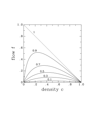
Figure 4: Fundamental diagram for the modified CA for different values of $p$.

References

References

- [1] K. Nagel and M. Schreckenberg, J. Phys. I (France) 2, 2221 (1992).
- [2] see the contributions of K. Nagel and T. Nagatani in these proceedings.
- [3] M. Schreckenberg, A. Schadschneider, K. Nagel and N. Ito, Phys. Rev. E 51, 2939 (1995).
- [4] A. Schadschneider and M. Schreckenberg, J. Phys. A: Math Gen. 26, L679 (1993).
- [5] A. Schadschneider and M. Schreckenberg, in preparation.
- [6] J.G. Brankov, V.B. Priezzhev, A. Schadschneider and M. Schreckenberg, to be published.
-
[7]
P.W. Kasteleyn, J. Math. Phys. 4, 287 (1963).