Mean-Field Nematic–Smectic-A Transition in a Random Polymer Network

Abstract

Liquid crystal elastomers present a rich combination of effects associated with orientational symmetry breaking and the underlying rubber elasticity. In this work we focus on the effect of the network on the nematic–smectic-A transition, exploring the additional translational symmetry breaking in these elastomers. We incorporate the crosslinks as a random field in a microscopic picture, thus expressing the degree to which the smectic order is locally frozen with respect to the network. We predict a modification of the NA transition, notably that it can be treated at the mean-field level (type-I system), due to the coupling with elastic degrees of freedom. There is a shift in the transition temperature $T_{\scriptscriptstyle NA}$, a suppression of the Halperin-Lubensky-Ma (HLM) effect (thus recovering the mean-field continuous transition to the smectic state), and a new tri-critical point, depending on the conditions of network formation. When the nematic phase possesses ‘soft elasticity’, the NA transition becomes of first order due to the coupling with soft phonons in the network. We also discuss the microscopic origin of phenomenological long-wavelength coupling between smectic phase and elastic strain.

I Introduction

Randomly crosslinked networks of polymer liquid crystal (LCP) materials (liquid crystalline elastomers and gels) have been a subject of substantial experimental and theoretical activity in recent years. A newcomer to this area can find out about about the synthesis of side-chain and main-chain systems, characteristic physical effects, and concepts related to the nematic state in review articles [1, 2]. Three major factors determine the behavior of these remarkable materials: liquid crystalline symmetry breaking; rubber elasticity coupled to the resulting anisotropy, producing a highly mobile principal axis; and, finally, randomly placed (and sometimes randomly oriented) network crosslinks. Random disorder introduced by these crosslinks encourages elastomers formed in the isotropic state to cool into polydomains, i.e. highly non-uniform textures of their liquid crystalline phases. If the network is formed in the presence of an external field, or in a uniform monodomain low-temperature phase, the resulting elastomer remains macroscopically uniform.

Smectic elastomers (refs. [3, 4, 5] represent a few recent examples) comprise liquid crystalline polymers crosslinked into a network which contains liquid crystalline groups ordered into a one-dimensional density wave, or a smectic state. One may consider either main chain or, more commonly, side-chain LCP’s. The smectic order is typically obtained by forming the network in a smectic state (e.g. by crosslinking at temperatures below the nematic–smectic-A, or NA, transition temperature $T^{0}_{\scriptscriptstyle\it NA}$ in the melt). It can also be obtained by cooling a sample that has been prepared in the nematic state through the transition temperature $T_{\scriptscriptstyle\it NA}$, where we expect $T_{\scriptscriptstyle\it NA}<T^{0}_{\scriptscriptstyle\it NA}$. The NA transition in networks is expected to be qualitatively very different from the same transition in melts because of the presence of elastic strain degrees of freedom and the local effects of random crosslinks.

In the conventional NA transition, the degrees of freedom are the smectic order parameter $\psi({\rm\bf r})$ and the director fluctuations $\delta\mathchoice{{\hbox{\boldmath$\displaystyle n$}}}{{\hbox{\boldmath$\textstyle n$}}}{{\hbox{\boldmath$\scriptstyle n$}}}{{\hbox{\boldmath$\scriptscriptstyle n$}}}$. The parameter $\psi({\rm\bf r})$ describes the departure of the mesogen center-of-mass density $\rho({\rm\bf r})$ from a uniform density $\rho_{0}$, in a form of single wavelength modulation [6, 7]

$$\rho({\rm\bf r})=\rho_{0}\left\{1+{1\over\sqrt{2}}\left[\psi({\rm\bf r})e^{i{\rm\bf q}_{0}\cdot{\rm\bf r}}+{\it c.c}\right]\right\}.$$ (1)

The nematic state is parameterized by the director $\textstyle\hat{n}$, which indicates the axis of preferential alignment of the mesogenic groups, and $\delta\mathchoice{{\hbox{\boldmath$\displaystyle\hat{n}$}}}{{\hbox{\boldmath$\textstyle\hat{n}$}}}{{\hbox{\boldmath$\scriptstyle\hat{n}$}}}{{\hbox{\boldmath$\scriptscriptstyle\hat{n}$}}}$ indicates the fluctuations of this axis. While the NA transition should be continuous according to symmetry arguments, director fluctuations may change this picture. Halperin, Lubensky, and Ma [8] argued that the coupling to the fluctuating “gauge” field $\delta\mathchoice{{\hbox{\boldmath$\displaystyle n$}}}{{\hbox{\boldmath$\textstyle n$}}}{{\hbox{\boldmath$\scriptstyle n$}}}{{\hbox{\boldmath$\scriptscriptstyle n$}}}$ should induce a first order transition in type-I smectics (and the analogous superconducting system). In type-I smectics the characteristic length for penetration of the director twist into the ordered smectic state is much smaller that the correlation length for the smectic order parameter, so that director fluctuations may be treated at a mean field level. Type-II smectics and superconductors, in which the gauge field fluctuations are correlated on length scales comparable or larger than that of the order parameter $\psi({\rm\bf r})$, require a more sophisticated analysis. The beliefs about the nature of this transition have varied over the years. A renormalization group $\epsilon$-expansion [8] yielded no fixed point for physical order parameters, suggesting that the transition is weakly first order. However, duality arguments combined with Monte Carlo calculations on a lattice [9] predicted a continuous transition in the universality class of the inverted 3D XY-transition (that is, the amplitude ratios are inverted), experiments have generally yielded a continuous transition of the non-inverted 3D XY class [10, 11, 12] (but see [13]). Toner [14] has argued, on the basis of a dislocation-melting theory, that the transition should be continuous; Andereck and Patton [15] have calculated critical exponents within self-consistent perturbation theory; and Radzihovsky [16] has performed a similar calculation for the analogous type-II superconducting transition, demonstrating the existence of a fixed point not found in $\epsilon$-expansion of [8].

While our understanding of the NA transition could be incomplete, the nature of the smectic state is well-understood. The smectic one-dimensional density wave, of wave number $q_{0}$, suffers the Landau-Peierls instability and the system exhibits quasi long ranged order (with an algebraic decay of density correlations at long distances) [17, 18]. The source of this instability is the Goldstone modes corresponding to the arbitrary phase of the smectic density wave, whose long wavelength free energy is given by the Landau-Peierls elastic energy of a one-dimensional solid [19]. In three dimensions this energy yields algebraic decay of correlations in the ordered state, analogous to systems with broken continuous symmetry in two dimensions.

In contrast to a liquid crystalline melt, a liquid crystalline elastomer has an additional set of long-wavelength degrees of freedom: the elastic deformation ${\rm\bf v}({\rm\bf r})$, defined by the local network displacement, ${\rm\bf r}\longrightarrow{\rm\bf r}+{\rm\bf v}({\rm\bf r})$. Smectic order couples to the elasticity through the crosslinks, and this coupling is manifested in two effects:

• Crosslinks pin the smectic phase and break translational invariance. The mesogens are either incorporated into the polymer backbone (main chain LCP’s) or tethered to the network (side chain LCP’s), and the stretching energy for relative translations between elastic displacements of the crosslinks $v_{z}({\rm\bf r})$ along the direction of the smectic density wave and the layer displacement $u({\rm\bf r})$ can be written phenomenologically as [20]

  $$2F_{d}=\Lambda\int\!d^{3}\!r[v_{z}({\bf r})-u({\bf r})]^{2}.$$ (2)

  This energy is defined on lengthscales of order or longer than the characteristic mesh size and, most importantly, is present for uniform relative translations. This coupling restores the Bragg peaks associated with smectic order [20]. In Section II we argue that this term is in fact only a metastable term, and the relative displacement $v_{z}({\bf r})-u({\bf r})$ may be relaxed by layer hopping [21] with a characteristic relaxation time.

• The preferential reduction of mesogen density around a crosslink due to, e.g., the steric exclusion of the mesogen, leads us (see Section II) to model the crosslinks by a local random field which adjusts the smectic phase:

  $$F_{\scriptscriptstyle RF}=\gamma\int\!d^{3}\!r\,c({\rm\bf r})|\psi({\rm\bf r})|\cos\left[q_{0}(z-u({\rm\bf r})+v_{z}({\rm\bf r}))\right],$$ (3)

  where $c({\rm\bf r})$ is the local crosslink concentration.

The smectic elastomer thus contains four contributions to the continuum free energy in addition to the smectic and nematic free energies associated with the NA transition in liquids. These are:

• The elastic free energy of a uniaxial solid [22], written in terms of the symmetric elastic strain $\epsilon_{\alpha\beta}=\frac{1}{2}(\nabla_{\alpha}v_{\beta}+\nabla_{\beta}v_{\alpha})$. This contribution describes the phonon field (in most elastomers - incompressible) in the rubbery network. It couples to the relevant variables of the NA transition through the following effects.

• Eq. (2), the term penalizing relative shifts in the smectic phase variable $u({\rm\bf r})$ and the phonon displacement parallel to it, $v_{z}({\rm\bf r})$.

• Rubber-nematic couplings [23], penalizing relative rotations of the elastic strain $\mathchoice{{\hbox{\boldmath$\displaystyle\Omega$}}}{{\hbox{\boldmath$\textstyle\Omega$}}}{{\hbox{\boldmath$\scriptstyle\Omega$}}}{{\hbox{\boldmath$\scriptscriptstyle\Omega$}}}=\frac{1}{2}(\nabla\times{\rm\bf v})$ and the nematic director, $\mathchoice{{\hbox{\boldmath$\displaystyle\omega$}}}{{\hbox{\boldmath$\textstyle\omega$}}}{{\hbox{\boldmath$\scriptstyle\omega$}}}{{\hbox{\boldmath$\scriptscriptstyle\omega$}}}=\mathchoice{{\hbox{\boldmath$\displaystyle\hat{n}$}}}{{\hbox{\boldmath$\textstyle\hat{n}$}}}{{\hbox{\boldmath$\scriptstyle\hat{n}$}}}{{\hbox{\boldmath$\scriptscriptstyle\hat{n}$}}}\times\delta\mathchoice{{\hbox{\boldmath$\displaystyle\hat{n}$}}}{{\hbox{\boldmath$\textstyle\hat{n}$}}}{{\hbox{\boldmath$\scriptstyle\hat{n}$}}}{{\hbox{\boldmath$\scriptscriptstyle\hat{n}$}}}$.

• The random field term, Eq. (3), describing the effect of crosslinks on the phase of the smectic order parameter.

In this work we consider the microscopic origin of Eq. (2) and treat the random field in Eq (3) by the replica formalism [24], with the following results [embodied in Eqs. (24)] for the mean-field theory of the NA transition in the network:

• Near the putative continuous NA transition Eq. (2) may be ignored, since it is primarily a dynamic effect. At low enough temperatures (when the characteristic timescale becomes essentially infinite) this term must be considered.

• At the mean field level nematic director fluctuations no longer induce the Halperin-Lubensky-Ma first order smectic phase transition: they acquire a mass which reduces their effect on the NA transition. The existence of this mass in fact makes the mean field treatment (and the associated type-I assumption) essentially exact.

• However, in the special case where the nematic elastomer possesses soft elasticity (see Eq. 11 below), characteristic of spontaneously breaking the symmetry from the isotropic to nematic states [25, 26], elastic strain fluctuations [the phonons ${\rm\bf v}({\rm\bf r})$] restore the HLM effect and the concomitant first order phase transition.

• If the nematic state is field-induced rather than spontaneous (i.e. the network has been formed to record the broken orientational symmetry), the corresponding network phonon modes are conventional and the type-I NA transition should be continuous. We predict a tri-critical point in the crossover region between these two regimes.

• The effect of disorder on the NA transition is a simple renormalization of the transition temperature $T_{\scriptscriptstyle NA}$. The transition temperature increases because crosslinks localize the smectic phase variable and encourage order in the disordered phase. However, slightly below $T_{\scriptscriptstyle NA}$ the smectic state crosses over to a ‘glassy’ state characterized by replica–symmetry-breaking.

• We emphasize that the typical nematic or smectic network is most likely to be ‘hard’, and that the ‘soft’ case we discuss extensively here is, for most practical cases, a theoretical construct which provides a framework for understanding the implications of a smectic state coupled to an underlying elastic continuum.

Our description of the NA transition in the network is mesoscopic because we treat the smectic and director degrees of freedom as smoothly varying fields while including the microscopic interaction of the crosslinks with the smectic order parameter. The calculation in this paper sets up the proper coarse-grained model with which to investigate the effects of disorder on the smectic network, which we discuss briefly here and in more detail in a forthcoming work. The coarse-grained nematic and smectic fields are defined on a length $\ell_{\it lc}$ of order a correlation length for liquid-crystalline fluctuations, while the elastic strain field is coarse-grained on lengths down to the mesh size $\ell_{\it x}$ in the network, which may be larger than $\ell_{\it lc}$. These different lengthscales must be kept in mind throughout.

This paper is organized as follows: in Section II we present a more detailed discussion of the two primary effects of the network-smectic couplings; in Section III we present the model free energy for the system; in Section IV we sketch the integration of the elastic strain and director fluctuations and present an effective free energy for the smectic in the presence of disorder; and we conclude in Section V. Our primary results are the effective Landau energies at the end of Section IV and the discussion in Section II about the smectic-elastic couplings. Our goal here is to understand the various terms in the Hamiltonian describing the NA transition, and identify the effects of disorder and rubber elasticity on the instability to the smectic state. We leave for the future a detailed analysis of the effects of disorder on the low temperature smectic state. The appendix contain some technical details of the replica calculations.

II Smectic–Elastic Couplings

A Random Field

In this section we justify the random field coupling, Eq. (3). This interaction represents the pinning of the smectic phase to network inhomogeneities, which we represent by a random distribution of crosslinks. Let us focus on side-chain LCP’s, Fig. 1, since these constitute the most commonly synthesized liquid crystalline elastomers. The three constituents of the elastomer are flexible backbone monomers, crosslink groups, and mesogenic side-groups attached to the backbone with flexible spacers. In elastomers (as opposed to tough and brittle densely-crosslinked resins) the volume fraction of crosslinks is much smaller than that of the backbone and mesogenic groups, typically less than a percent of the aggregate. Hence we treat the environment of the mesogens as a uniform mesogen/backbone mixture with interspersed crosslink groups.

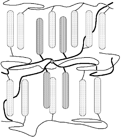
FIG. 1.: Sketch of mesogenic groups in a smectic elastomer.

It is reasonable to expect a steric repulsion between the mesogen and the crosslink which is enhanced relative to the steric repulsion between the backbone and the mesogen, simply because four chains come together at the crosslink. The presence of a Flory-$\chi$ parameter between the mesogen and backbone groups contributes a similar effect. While there will also be an interaction with the local nematic order, since the mesogens may adopt an alignment dictated by the crosslink, we concentrate in this work on the effects of disorder on a smectic phase appearing out of a uniform conventional nematic state. Hence, we model the crosslinks by a local random field which induces smectic order and fixes the smectic phase, leading to Eq. (3). The corresponding energy contribution for each crosslink in the smectic potential is

$$F_{\scriptscriptstyle RF}=\sum_{i}\gamma|\psi({\rm\bf R}_{i})|\cos\left[q_{0}(z_{i}-u({\rm\bf R}_{i}))\right]\ ,$$ (4)

where ${\rm\bf R}_{i}$ is the position of the $i^{\rm th}$ crosslink. The coupling constant $\gamma$ can be estimated on the basis of Fig. 1. We shall assume that the crosslinking point localizes the positions of $\phi$ monomers (with $\phi$ the crosslink functionality). The barrier for such an object to ‘tunnel’ through a smectic smectic layer is a molecular characteristic of the material describing the degree of miscibility of backbone and the mesogenic side-groups, and is roughly of order $\phi\chi$, where $\chi$ is the the Flory-$\chi$ parameter between mesogens and backbone, which includes both steric and energetic interactions.

Introducing the continuum crosslink density $c({\rm\bf r})=\sum_{i}\delta({\rm\bf r}-{\rm\bf R}_{i})$, so that under an elastic distortion ${\rm\bf R}_{i}\rightarrow{\rm\bf R}_{i}+{\rm\bf v}$ they distort by $c({\rm\bf r})\rightarrow c({\rm\bf r}-{\rm\bf v})$, we can transform (4) to collective variables. After changing variables ${\rm\bf r}^{\prime}={\rm\bf r}-{\rm\bf v}({\rm\bf r})$ we obtain

$$F_{\scriptscriptstyle RF} = \gamma\int\!d^{3}\!r\,c({\rm\bf r})\,|\psi({\rm\bf r}+{\rm\bf v}({\rm\bf r}))|\cos\left[q_{0}\left(z-u({\rm\bf r})+v_{z}({\rm\bf r})\right)\right].$$ (5)

(Changing variables in the argument of $u({\rm\bf r})$ introduces higher-order gradient corrections which are irrelevant in a mean-field treatment).

Rather than working with the discrete crosslink positions, we represent the crosslink concentration $c({\rm\bf r})$ by a Gaussian probability distribution [27]:

$$P[c]\propto\exp\left\{-\frac{1}{2}\int\!d^{3}\!r\,\frac{c({\rm\bf r})^{2}}{2N_{x}}\right\}\ ,$$ (6)

where $N_{x}$ is number of crosslinks per unit volume of the system. For this random distribution of crosslinks the characteristic moments are $\langle c({\rm\bf r})\rangle=N_{x}$  and  $\langle c({\rm\bf r})c({\rm\bf r}^{\prime})\rangle=N_{x}\delta({\rm\bf r}-{\rm\bf r}^{\prime})$.

One should note, at this point, that a different situation emerges for a network formed in a deep uniform smectic phase: the polymer backbone in such a system is highly constrained between the smectic layers and, therefore, the crosslink distribution (6) has a positionally modulated kernel. This possibility will have a profound effect on the phase ordering in the smectic phase, but is not relevant for the NA transition description we are concerned here. Also, in a physical system crosslinks fluctuate about their mean positions [28], which broadens the kernel of Eq.(6) into a Gaussian distribution with a width (in real space) proportional to the extent of the typical crosslink fluctuation. We ignore such fluctuation effects for now.

B Translational Invariance

The second effect of the network on the smectic phase is due to stretching the polymer backbone. This leads to a free energy cost for uniformly displacing the smectic phase relative to the elastic displacement, given by Eq.(2) [20]. Whereas the contribution of the previous sub-section acts only at the crosslink position, the stretching effect influences the smectic phase all along the strand between crosslinks, and is coarse-grained at the mesh size or larger. To understand this in detail we first note the distinction between the smectic phase variable $q_{0}u$ and the $z$-displacement $\eta_{i}$ of the center-of-mass of the $i^{th}$ smectic mesogen.

The phase $q_{0}u$ is a coarse-grained variable and the displacements $\{\eta_{i}\}$ are microscopic variables. To calculate the position of the smectic phase from a microscopic picture one must, in principle, average over all the positions of the mesogens. In an equilibrium smectic liquid the mesogens lie in a smectic potential given by, for example, a cosine modulation [29], but are not fixed in one trough of this potential: rather, they fluctuate back and forth over the barriers. In a strongly-ordered smectic state the activation over the barriers is very rare, while in a weak smectic state these fluctuations are quite common. The ‘motion’ of the smectic phase thus corresponds to the average motion of the mesogens’ centers-of-mass.

Now consider an elastomer in a smectic state and imagine displacing the smectic phase while fixing the crosslink positions. For clarity we focus on a side-chain liquid crystalline network, but the argument applies to a main-chain network as well. The displacement of the smectic phase displaces the average positions $\{\eta_{i}\}$ of the mesogenic sidegroups. Since these are tethered to the polymer backbone, this costs roughly the entropy of displacing the center-of-mass of a polymer chain a distance $u$ while keeping the endpoints (i.e. crosslink positions) fixed. A simple calculation leads to an energy per chain of $V_{u}\sim k_{\scriptscriptstyle B}Tu^{2}/(Na^{2})$, with $N$ the number of monomers of size $a$ between crosslinks. In addition to this elastic force, an individual mesogen feels a force due to the smectic potential [29]. At zero temperature this potential enforces the separation of the smectic phase variable and the crosslink displacement, but at finite temperature this barrier may be overcome by hopping. By hopping we mean that the mesogen flips from one smectic trough to another, in such a way as to relax the strain. This allows the smectic phase variable to increase without bound while roughly localizing the mesogens’ centers-of-mass.

Hence a timescale $\tau^{\ast}$ separates liquid-like smectic behavior at long times from ‘solid-like’ smectic behavior at short times, the latter characterized by the elastic modulus $\Lambda$. For temperatures above the nematic-smectic transition temperature $\tau^{\ast}$ is extremely small and we may ignore this elastic effect. However, as the network is cooled deep into the smectic state $\tau^{\ast}$ grows, and for all practical purposes we must include this term. Since we are only concerned here with very weak smectic phases in this work, we leave further discussion of the interesting dynamics of a smectic network to another work.

III The model

In this section we introduce the full free energy of the system, and set up the replica calculation. The NA transition in a liquid is described by the Landau-de Gennes free energy,

$$2F_{\scriptscriptstyle\it NA}=\int\!d^{3}\!r\,\left\{\tau|\psi({\rm\bf r})|^{2}+\frac{1}{2}\beta|\psi({\rm\bf r})|^{4}+g_{\perp}|(\mathchoice{{\hbox{\boldmath$\displaystyle\nabla$}}}{{\hbox{\boldmath$\textstyle\nabla$}}}{{\hbox{\boldmath$\scriptstyle\nabla$}}}{{\hbox{\boldmath$\scriptscriptstyle\nabla$}}}_{\perp}-iq_{0}\delta\mathchoice{{\hbox{\boldmath$\displaystyle\hat{n}$}}}{{\hbox{\boldmath$\textstyle\hat{n}$}}}{{\hbox{\boldmath$\scriptstyle\hat{n}$}}}{{\hbox{\boldmath$\scriptscriptstyle\hat{n}$}}})\psi({\rm\bf r})|^{2}+g_{\parallel}|\partial_{z}\psi({\rm\bf r})|^{2}\right\},$$ (7)

where the minimal coupling $(\mathchoice{{\hbox{\boldmath$\displaystyle\nabla$}}}{{\hbox{\boldmath$\textstyle\nabla$}}}{{\hbox{\boldmath$\scriptstyle\nabla$}}}{{\hbox{\boldmath$\scriptscriptstyle\nabla$}}}_{\perp}-iq_{0}\delta\mathchoice{{\hbox{\boldmath$\displaystyle\hat{n}$}}}{{\hbox{\boldmath$\textstyle\hat{n}$}}}{{\hbox{\boldmath$\scriptstyle\hat{n}$}}}{{\hbox{\boldmath$\scriptscriptstyle\hat{n}$}}})$ satisfies rotational invariance of the director and the layered system [7]. In the high-temperature nematic phase director distortions $\delta\mathchoice{{\hbox{\boldmath$\displaystyle\hat{n}$}}}{{\hbox{\boldmath$\textstyle\hat{n}$}}}{{\hbox{\boldmath$\scriptstyle\hat{n}$}}}{{\hbox{\boldmath$\scriptscriptstyle\hat{n}$}}}$ are penalized by the Frank free energy,

$$2F_{\it fr}=\int\!d^{3}\!r\,\left\{K_{1}(\mathchoice{{\hbox{\boldmath$\displaystyle\nabla$}}}{{\hbox{\boldmath$\textstyle\nabla$}}}{{\hbox{\boldmath$\scriptstyle\nabla$}}}{{\hbox{\boldmath$\scriptscriptstyle\nabla$}}}\!\cdot\!\delta{\bf\hat{n}})^{2}+K_{2}({\bf\hat{n}}\!\cdot\!\mathchoice{{\hbox{\boldmath$\displaystyle\nabla$}}}{{\hbox{\boldmath$\textstyle\nabla$}}}{{\hbox{\boldmath$\scriptstyle\nabla$}}}{{\hbox{\boldmath$\scriptscriptstyle\nabla$}}}\!\times\!\delta{\bf\hat{n}})^{2}+K_{3}({\bf\hat{n}}\!\times\!\mathchoice{{\hbox{\boldmath$\displaystyle\nabla$}}}{{\hbox{\boldmath$\textstyle\nabla$}}}{{\hbox{\boldmath$\scriptstyle\nabla$}}}{{\hbox{\boldmath$\scriptscriptstyle\nabla$}}}\!\times\!\delta{\bf\hat{n}})^{2}\right\}.$$ (8)

In this work we use the one constant approximation, $K_{1}=K_{2}=K_{3}\equiv K$. The elastic energy of an underlying uniaxial solid can be written in many ways [22], and we choose the representation through the traceless strain tensor $\bar{\epsilon}_{\alpha\beta}\equiv\epsilon_{\alpha\beta}-\frac{1}{3}{\rm Tr}[\mathchoice{{\hbox{\boldmath$\displaystyle\epsilon$}}}{{\hbox{\boldmath$\textstyle\epsilon$}}}{{\hbox{\boldmath$\scriptstyle\epsilon$}}}{{\hbox{\boldmath$\scriptscriptstyle\epsilon$}}}]\delta_{\alpha\beta}$, in order to deal explicitly with the case of a nearly incompressible network:

$$2F_{\it el}=\int\!d^{3}\!r\,\left\{C_{1}\bar{\epsilon}_{zz}^{2}+2C_{2}\bar{\epsilon}_{zz}{\rm Tr}[\mathchoice{{\hbox{\boldmath$\displaystyle\epsilon$}}}{{\hbox{\boldmath$\textstyle\epsilon$}}}{{\hbox{\boldmath$\scriptstyle\epsilon$}}}{{\hbox{\boldmath$\scriptscriptstyle\epsilon$}}}]+C_{3}\left({\rm Tr}[\mathchoice{{\hbox{\boldmath$\displaystyle\epsilon$}}}{{\hbox{\boldmath$\textstyle\epsilon$}}}{{\hbox{\boldmath$\scriptstyle\epsilon$}}}{{\hbox{\boldmath$\scriptscriptstyle\epsilon$}}}]\right)^{2}+2C_{4}(\bar{\epsilon}_{xx}^{2}+2\bar{\epsilon}_{xy}^{2}+\bar{\epsilon}_{yy}^{2})+4C_{5}(\bar{\epsilon}_{xz}^{2}+\bar{\epsilon}_{yz}^{2})\right\},$$ (9)

where the $\hat{z}$-axis is chosen along the nematic director. In the isotropic case, the elastic moduli $\{C_{i}\}$ transform to the Lamé coefficients as $C_{1}=2\mu\,;\ C_{2}=0\,;\ C_{3}=\lambda+\frac{2}{3}\mu\,$ and $\,C_{4}=C_{5}=\mu$. In most cases we take the limit $C_{3}\rightarrow\infty$, since $\lambda/\mu\sim 10^{4}-10^{5}$ in a typical rubber. The rubber shear moduli scale as $\mu\sim N_{x}k_{\scriptscriptstyle B}T$, where $N_{x}\sim\ell_{x}^{-2}$ is the number of crosslinks per unit volume.

The rubber–nematic free energy penalizing relative rotations of the director $\mathchoice{{\hbox{\boldmath$\displaystyle\omega$}}}{{\hbox{\boldmath$\textstyle\omega$}}}{{\hbox{\boldmath$\scriptstyle\omega$}}}{{\hbox{\boldmath$\scriptscriptstyle\omega$}}}=\mathchoice{{\hbox{\boldmath$\displaystyle\hat{n}$}}}{{\hbox{\boldmath$\textstyle\hat{n}$}}}{{\hbox{\boldmath$\scriptstyle\hat{n}$}}}{{\hbox{\boldmath$\scriptscriptstyle\hat{n}$}}}\times\delta\mathchoice{{\hbox{\boldmath$\displaystyle\hat{n}$}}}{{\hbox{\boldmath$\textstyle\hat{n}$}}}{{\hbox{\boldmath$\scriptstyle\hat{n}$}}}{{\hbox{\boldmath$\scriptscriptstyle\hat{n}$}}}$ and elastic strain $\mathchoice{{\hbox{\boldmath$\displaystyle\Omega$}}}{{\hbox{\boldmath$\textstyle\Omega$}}}{{\hbox{\boldmath$\scriptstyle\Omega$}}}{{\hbox{\boldmath$\scriptscriptstyle\Omega$}}}=\frac{1}{2}(\nabla\times{\rm\bf v})$ can be written as [23, 26]

$$2F_{\it n-u}=\int\!d^{3}\!r\,\left\{b_{1}\left[(\mathchoice{{\hbox{\boldmath$\displaystyle\Omega$}}}{{\hbox{\boldmath$\textstyle\Omega$}}}{{\hbox{\boldmath$\scriptstyle\Omega$}}}{{\hbox{\boldmath$\scriptscriptstyle\Omega$}}}-\mathchoice{{\hbox{\boldmath$\displaystyle\omega$}}}{{\hbox{\boldmath$\textstyle\omega$}}}{{\hbox{\boldmath$\scriptstyle\omega$}}}{{\hbox{\boldmath$\scriptscriptstyle\omega$}}})\!\times\!{\bf\hat{n}}\right]^{2}+2b_{2}\,{\bf\hat{n}}\!\cdot\!\mathchoice{{\hbox{\boldmath$\displaystyle\epsilon$}}}{{\hbox{\boldmath$\textstyle\epsilon$}}}{{\hbox{\boldmath$\scriptstyle\epsilon$}}}{{\hbox{\boldmath$\scriptscriptstyle\epsilon$}}}\!\cdot\!(\mathchoice{{\hbox{\boldmath$\displaystyle\Omega$}}}{{\hbox{\boldmath$\textstyle\Omega$}}}{{\hbox{\boldmath$\scriptstyle\Omega$}}}{{\hbox{\boldmath$\scriptscriptstyle\Omega$}}}-\mathchoice{{\hbox{\boldmath$\displaystyle\omega$}}}{{\hbox{\boldmath$\textstyle\omega$}}}{{\hbox{\boldmath$\scriptstyle\omega$}}}{{\hbox{\boldmath$\scriptscriptstyle\omega$}}})\!\times\!{\bf\hat{n}}\right\},$$ (10)

where $b_{1}$ and $b_{2}$ are proportional to, respectively, the nematic order parameter $Q^{2}$ and $Q$, multiplied by $N_{x}k_{\scriptscriptstyle B}T$. A positive coupling $b_{2}$ corresponds to a network which favors parallel alignment between mesogen and backbone orientations, while a negative $b_{2}$ favors perpendicular alignment.

For the special case of nematic elastomers which possess an arbitrary choice of the nematic axis (because of a spontaneously broken symmetry of a network, formed in the isotropic state) rather than a ‘quenched’ axis of alignment dictated by, for example, an applied field during crosslinking or crosslinking in the nematic state, the relationship $C_{5}-b_{2}^{2}/(4b_{1})=0$ holds [25, 26] and the phonons described by $\bar{\epsilon}_{xz}$ and $\bar{\epsilon}_{yz}$ are “soft” (i.e. the corresponding phonons have fluctuation spectrum $\langle|u(q)|^{2}\rangle\sim q^{-4}$ instead of the conventional $q^{-2}$ behavior). The deviation of the network from this curious soft case is thus parameterized by

$$C_{5}-{b_{2}^{2}\over 4b_{1}}\equiv\Delta.$$ (11)

The presence or absence of these modes plays an essential role in describing the NA transition. While a perfect soft nematic elastomer ($\Delta=0$) is unlikely to be found in typical experiments due to random stresses in the nematic state or a predetermined alignment direction during network formation, we include the soft case to present a complete theoretical picture.

The partition function for the system is then given by

$${\cal Z\/}=\int\!{\cal D\/}\psi{\cal D}{\rm\bf v}{\cal D}\delta\mathchoice{{\hbox{\boldmath$\displaystyle\hat{n}$}}}{{\hbox{\boldmath$\textstyle\hat{n}$}}}{{\hbox{\boldmath$\scriptstyle\hat{n}$}}}{{\hbox{\boldmath$\scriptscriptstyle\hat{n}$}}}\ \exp-{1\over k_{\scriptscriptstyle B}T}\bigl{\{}F_{\scriptscriptstyle NA}+F_{\it fr}+F_{\it el}+F_{\it n-u}+F_{\scriptscriptstyle RF}\bigr{\}}.$$ (12)

To find the effects of crosslinks on the NA transition in the network and, eventually, on the nature of the smectic state, we average over the disorder associated with these crosslinks. To compute quantities such as the quenched disorder-averaged free energy and correlation functions we use the replica trick [24] to write the free energy of the system as

$$F/k_{\scriptscriptstyle B}T=-\langle\log{\cal Z\/}\rangle_{P}=\lim_{n\rightarrow 0}{1-\langle{\cal Z\/}^{n}\rangle_{P}\over n},$$ (13)

introducing $n$ replicas of the system. The disorder average over the distribution $P[c]$, Eq. (6), couples the replicas together into the term $F_{\it repl}$:

$$2F_{\it repl} = -\frac{\gamma^{2}N_{x}}{k_{\scriptscriptstyle B}T}\sum_{a,b=1}^{n}\int\!d^{3}\!r\,|\psi^{a}({\rm\bf r}+{\rm\bf v}^{a}({\rm\bf r}))||\psi^{b}({\rm\bf r}+{\rm\bf v}^{b}({\rm\bf r}))|$$ (15)

$$\ \ \ \times\,\cos\left[q_{0}\left(z-u^{a}({\rm\bf r})+v_{z}^{a}\left({\rm\bf r}\right)\right)\right]\,\cos\left[q_{0}\left(z-u^{b}({\rm\bf r})+v_{z}^{b}({\rm\bf r})\right)\right]\,.$$

Note that $u$ fluctuations are implicitly included in the measure for $\psi$ fluctuations. From here on we consider a uniform $\psi$ for the purposes of understanding the mean-field behavior of the transition, and as such will not consider fluctuations of its phase.

We next coarse-grain the system by averaging over the period of the smectic modulation $q_{0}^{-1}$ along the layer normal $z$. This procedure requires that both the ‘mean-free-path’ between crosslinks $\ell_{x}\sim N_{x}^{-1/2}$ and typical length scale of the relative translations $u({\rm\bf r})-v_{z}({\rm\bf r})$ be large compared to the layer spacing $2\pi q_{0}^{-1}$. We find

$$F_{\it repl}=-\Gamma\sum_{a,b=1}^{n}\int\!d^{3}\!r\,|\psi^{a}||\psi^{b}|\cos\left[q_{0}\left(v^{a}({\rm\bf r})-v^{b}({\rm\bf r})\right)\right],$$ (16)

where $\Gamma=\gamma^{2}N_{x}/(2k_{\scriptscriptstyle B}T)$. The free energy of the system is now given by Eq. (13), with $n$ replicated copies of the partition function Eq. (12), with $F_{\scriptscriptstyle\mit RF}$ replaced by $F_{\mit repl}$. Note that the similar form of the replica Hamiltonian, containing a translationally invariant cosine of fluctuating field $(v^{a}-v^{b})$, appears in the problem of random flux pinning in superconductors [30].

IV Mean Field Phase Behavior

To see the effect of the crosslinks on the NA transition in the network we integrate out the strain and director fluctuations and examine the stability of the resulting effective theory for a uniform $|\psi|$. This procedure is valid when the penetration length $\lambda$ for director twist into the smectic is much smaller than the smectic coherence length $\xi=(g_{\perp}/\tau)^{1/2}$ (this situation is often referred to as the type-I smectic-A, by analogy with superconductors) [8]. For an elastic network, nematic fluctuations have a “mass” $m\approx q_{0}^{2}g_{\perp}|\psi|^{2}+b_{1}\Delta/C_{5}$, where the first term is the mass of due to smectic fluctuations and the second term, $\sim N_{x}k_{\scriptscriptstyle B}T$, is due to the coupling to the elastic network. As the transition is approached we have $|\psi|^{2}\sim\beta/\tau$ and the twist penetration length is given by $\lambda=(K/m)^{1/2}$, so that

$${\lambda\over\xi}=\left({\tau K\over\tau q_{0}^{2}g_{\perp}^{2}+g_{\perp}\Delta}\right)^{1/2}.$$ (17)

This Ginzburg parameter vanishes as the critical point is approached ($\tau\rightarrow 0$), so that the condition for a type-I smectic ($\lambda/\xi\ll 1$) is trivially satisfied and the mean-field treatment here is exact. [Note that for the perfect soft system, $\Delta=0$, the system may or may not be type-II, as with ordinary smectics.] Elastic fluctuations enter the theory at Gaussian level and may be integrated out at a mean-field level. A self-consistent check on the neglect of these fluctuations is to ensure the smectic correlation length at the fluctuation-induced first order transition is of order or larger than both the mesh size (to satisfy the coarse-graining procedure) and the twist penetration length.

To perform the calculations we choose a convenient geometry (cf. [6]). We decompose the displacement into

$${\rm\bf v}=(v_{z},v_{\perp},v_{t}),$$ (18)

where $v_{z}$ is parallel to the nematic director; $v_{\perp}$ is normal to the director and belongs to the plane defined by the director and the wavevector ${\rm\bf q}$ in Fourier space; and $v_{t}$ is in the direction defined by ${\rm\bf q}\times\mathchoice{{\hbox{\boldmath$\displaystyle\hat{n}$}}}{{\hbox{\boldmath$\textstyle\hat{n}$}}}{{\hbox{\boldmath$\scriptstyle\hat{n}$}}}{{\hbox{\boldmath$\scriptscriptstyle\hat{n}$}}}$. Similarly, $\delta\mathchoice{{\hbox{\boldmath$\displaystyle\hat{n}$}}}{{\hbox{\boldmath$\textstyle\hat{n}$}}}{{\hbox{\boldmath$\scriptstyle\hat{n}$}}}{{\hbox{\boldmath$\scriptscriptstyle\hat{n}$}}}=(\delta\hat{n}_{t},\delta\hat{n}_{\perp})$. Integrating out the director fluctuations is straightforward since they are not involved in the random coupling, and we find

$$\langle{\cal Z\/}^{n}\rangle_{P}=\int\!\prod_{a=1}^{n}{\cal D\/}\psi^{a}{\cal D}{\rm\bf v}^{a}\exp-{1\over k_{\scriptscriptstyle B}T}\left\{\sum_{a}\left[F_{1}\left(\psi^{a}\right)+\tilde{F}_{\it el}\left({\rm\bf v}^{a},\psi^{a}\right)\right]+F_{\it repl}\right\}.$$ (19)

The effective smectic free energy density is renormalized to

$${F_{1}(\psi)\over V}=\frac{1}{2}\tau|\psi|^{2}+\frac{1}{4}\beta|\psi|^{4}+k_{\scriptscriptstyle B}T\int_{\bf q}\,\log\Bigl{[}b_{1}+D_{0}(\psi)+Kq^{2}\Bigr{]}\ ,$$ (20)

where $V$ is the system volume and we have used the one-constant approximation for the bare Frank elastic constants Here and below, $\int_{\bf q}\equiv\int d^{3}q/(2\pi)^{3}$. The parameter $D_{0}=|\psi|^{2}g_{\perp}q_{0}^{2}$ is proportional to the square of the smectic order parameter, and the logarithm in Eq. (20) is the determinant of the quadratic form from integrating the director fluctuations. The factor $D_{0}(\psi)$ in this term gives rise to the Halperin-Lubensky-Ma effect in a mean-field type-I system. That is, when the director is not coupled to the network ($b_{1}=0$), director fluctuations are massless and the $q$-integration renormalizes the transition temperature $T_{\scriptscriptstyle NA}$, and yields a negative cubic term which induces a first order transition [8]. However, massive director fluctuations ($b_{1}\neq 0$) imply only even powers of $|\psi|$ in the expansion of the integral, destroying the HLM effect.

Eliminating $\delta\mathchoice{{\hbox{\boldmath$\displaystyle\hat{n}$}}}{{\hbox{\boldmath$\textstyle\hat{n}$}}}{{\hbox{\boldmath$\scriptstyle\hat{n}$}}}{{\hbox{\boldmath$\scriptscriptstyle\hat{n}$}}}$ also renormalizes the rubber elasticity, yielding $\tilde{F}_{\it el}$, which is a quadratic form in the phonon variable ${\rm\bf v}$. Together with $F_{\mit repl}$, the effective energy governing the elastic degrees of freedom is given by

$${\cal H}=\sum_{a}\tilde{F}_{\it el}+F_{\it repl}=\frac{1}{2}\sum_{a}\int_{\bf q}{\bf v}^{a}({\rm\bf q})\!\cdot\!{\bf M}(q,\psi)\!\cdot\!{\bf v}^{a}({\rm\bf-q})-\Gamma\sum_{a,b}\int\!d^{3}\!r|\psi^{a}||\psi^{b}|\cos q_{0}(v_{z}^{a}-v_{z}^{b}),$$ (21)

where the kernel matrix ${\bf M}(q,\psi)$ in $\tilde{F}_{\mit el}$ is given in the Appendix.

The next step is to integrate out the phonon variable ${\rm\bf v}({\rm\bf r})$ and extract the effective free energy as a function only of $\psi$. Since ${\cal H\/}$ is non-Gaussian this is a non-trivial step. We perform this integration by applying the Gaussian Variational Method (GVM) as introduced by Mezard and Parisi [31] for random systems with translationally invariant (in replica space) Hamiltonians, like our $\cos[v^{a}-v^{b}]$. In performing this integration we assume replica symmetry for the phonon fluctuations, which holds for small enough $\psi$ and is thus justified for an analysis of a continuous transition. We also assume replica symmetry in the value of $\psi$ which extremizes the partition function, so that we present below an effective free energy of $\psi$ which does not involve replicas and which we believe describes the NA transition in a random network.

The integration of ${\rm\bf v}$ is sketched in the Appendix, and yields two distinct theories, depending on whether or not the system exhibits ‘soft’ elasticity ($\Delta=0$). The effective free energies are:

$${F_{\psi}\over V} = \left\{\begin{array}[]{lr}\frac{1}{2}{\tau}_{0}|\psi|^{2}-\lambda_{0}|\psi|^{3}+\frac{1}{4}{\beta}_{0}|\psi|^{4}&\qquad(\Delta=0)\\ \vskip 6.0pt\cr\frac{1}{2}{\tau}_{\Delta}|\psi|^{2}+\frac{1}{4}{\beta}_{\Delta}|\psi|^{4}&(\Delta\neq 0)\end{array}\right.$$ (24)

which can also be presented as a single crossover expression covering both cases:

$${F_{\psi}\over V}=\frac{1}{2}\tilde{\tau}(\Delta)|\psi|^{2}+\tilde{\lambda}(\Delta,\psi)+\frac{1}{4}\tilde{\beta}(\Delta)|\psi|^{4}$$ (25)

The free energies above comprise one of the primary results of this work. In Eq. (25) the coefficients $\tilde{\tau}(\Delta)$ and $\tilde{\beta}(\Delta)$ are continuous analytic functions of $\Delta$, while $\tilde{\lambda}(\Delta,\psi)$ is a non-analytic function which gives the cubic term for $\Delta=0$. This term is responsible for the qualitative results we find. In this work we give only the detailed expression for the cubic crossover function $\tilde{\lambda}(\Delta,\psi)$, since this term alone determines the qualitative aspects of the transition.

Soft nematic elastomers ($\Delta=0$)—The renormalized coefficient ${\tau}_{0}$ has the form $\tilde{\tau}_{0}(T-T_{\scriptscriptstyle NA})$, with the new transition temperature shifted by the effects of rubber elasticity and random pinning (16). Besides this obvious effect, the new feature of this soft regime is the cubic term, which restores the HLM effect. This term is given by

$$\lambda_{0}=-{1\over 12\pi}\left({q_{0}^{2}g_{\perp}\over K}\right)^{3/2},$$ (26)

and is precisely the cubic term given by Halperin-Lubensky-Ma [8]. Hence, while the coupling of elasticity to the director (or gauge) field destroys the HLM effect, the effect is restored if the coupling preserves the set of Goldstone modes present in the nematic state, an intuitively pleasing situation.

Conventional nematic elastomers ($\Delta\neq 0$)—In a network formed in the nematic state there are no soft elastic phonons and no Goldstone modes, and the effective Landau-de Gennes free energy $F_{\psi}$ contains renormalized quadratic and quartic coefficients. There are numerous contributions to the quartic terms, but the qualitative nature of the renormalized quartic follows from examining the behavior of the non-analytic crossover function, given by

$$\tilde{\lambda({\Delta},\psi)} = -{1\over 12\pi K^{3/2}}\left[g_{\perp}q_{0}^{2}|\psi|^{2}+{4\Delta b_{1}^{2}\over 4\Delta b_{1}+(b_{1}+b_{2})^{2}}\right]^{3/2}$$ (27)

$$\simeq -{1\over 12\pi K^{3/2}}\left[{\cal O\/}(1,|\psi|^{2})+\frac{3}{8}g_{\perp}^{2}q_{0}^{4}{b_{1}+b_{2}\over b_{1}}{|\psi|^{4}\over\Delta^{1/2}}+\ldots\right],\quad\left({g_{\perp}q_{0}^{2}|\psi|^{2}\over b_{1}}<{4\Delta b_{1}\over(b_{1}+b_{2})^{2}}\ll 1\right),$$ (28)

where the first inequality defines the validity of expanding the $3/2$ power, and the second inequality allows us to simplify the results for a nearly-soft system ($\Delta\simeq 0$).

Hence, the non-analytic term yields a negative quartic coefficient when expanded for small $|\psi|$ at non-zero $\Delta$. For small enough $\Delta$ this term becomes very large and the expansion is only relevant for extremely small $|\psi|$. At the point where the expansion becomes invalid the quartic term must be replaced by a cubic term, and a tricritical point results. Alternatively, one may examine the free energy above, Eq. (25), to find a tricritical point at $\Delta_{\ast}$ given (for small $\Delta$) by

$$\beta_{\Delta_{\ast}}\approx\beta-{1\over 32\pi}\left({g_{\perp}q_{0}^{2}\over\Delta_{\ast}K^{3}}\right)^{1/2}{b_{1}+b_{2}\over b_{1}},$$ (29)

where $\beta$ is the bare quartic coefficient. The NA transition is of second (first) order for positive (negative) $\beta_{\Delta}$.

Thus, for small enough $\Delta$ the transition is expected to be of first order. This correction is most important in those systems which are already close to a tricritical point, $\beta\gtrsim 0$ [typically those with a relatively small nematic range, $T_{\scriptscriptstyle IN}-T_{\scriptscriptstyle NA}$, where $T_{\scriptscriptstyle IN}$ is the isotropic-nematic transition temperature [29, 7]]. We have checked numerically that, for a wide range of realistic elastic constants, the correction to $\beta$ ranges up to $0.1\,k_{\scriptscriptstyle B}Tq_{c}^{3}\sim\beta$, where $q_{c}$ is the microscopic (large wavenumber) cutoff that defines the coarse-graining of the theory [7]. As noted in the Appendix, the only effect of disorder is to slightly increase the transition temperature, which is sensible because crosslink sites locally enhance the smectic order. Our effective free energy assumes a replica-symmetric ground state. In the Appendix we note that the replica-symmetric solution is stable for $|\psi|=0$, while in the smectic state there is a crossover at small $|\psi|$ to a replica–non-symmetric state, which in this context refers to the effect of the smectic order on the background phonon spectrum. An analysis of the further effects of disorder on the low temperature state is beyond this scope of this work.

V Conclusion

A Experimental consequences

We conclude by first discussing some experimental consequences and signatures of this work. The primary qualitative prediction concerns the order of the transition. The preparation of networks of varying degrees of ‘softness’ (which may be controlled by, for example, changing the degree of order which is frozen into the smectic state) allow for tests of the predicted tricritical behavior between first- and second-order nematic–smectic-A transitions, which may be probed by, for example, specific heat experiments.

It would also be interesting to test the crossover to a ‘glassy’ phase characterized by replica-symmetry breaking. X-ray scattering to probe the smectic density wave should yield this information, in the form of a crossover from a Landau-Peierls’ form to a structure factor with temperature-independent logarithmic correlations, similar to the vortex glass considered by Korshunov [32] and Giamarchi and Le Doussal [33].

A cornerstone of our treatment involves the coupling between the smectic phase variable and the elastic strain, in Eq. (2), which we have asserted to be a dynamic effect. A signature of this would be a characteristic timescale $\tau^{\ast}$ associated with hopping of mesogens over the smectic barrier. In strong smectic phases this timescale should be essentially infinite so that we may use Eq. (2), but it should be present in weak smectics and emerge in measurements of the complex rheological response function.

B Critique and outlook

In this work we have examined the onset of the nematic–smectic-A transition in a smectic elastomer, and delineated two types of behavior (summarized in the free energies, Eqs. 24). Soft nematic elastomers should display a first order transition, due to the HLM effect induced by the spectrum of Goldstone modes which are a combination of director and strain fluctuations. Conventional ‘hard’ elastomers, on the other hand, should have a continuous transition, with a tricritical point as the soft limit is approached.

In performing our calculations we have assumed the system is in the type-I limit, so that a mean field treatment is valid. Since director fluctuations have an additional mass due to the coupling to the elastic network, we believe this limit is safe for smectic elastomers. We have treated disorder within the replica formalism and found that, at the level of the onset of the transition, the only effect is to stabilize the smectic state. A preliminary analysis suggests that the effects of disorder are certainly important deep in the smectic state.

Hence a natural extension of this work concerns the nature of the low temperature phase. The effects of disorder are two-fold: (1) Translational symmetry is broken and the smectic phase is locally pinned to the disorder, which should destroy the Landau-Peierls transition in favor of true long-range order of the smectic density wave; and (2) disorder can be strong enough to destroy the long-range order itself. Which, if either, of these effects wins out is an interesting question, analogous to the effects of disorder on other systems with continuous symmetry, such as the XY-model or flux lattices in superconductors.

A second, more speculative, result of our work is the suggestion that the coupling proposed previously to describe the energy penalty for sliding the smectic phase relative to the crosslinks, Eq. (2), is actually present only when one considers sufficiently short timescales (which, practically, may still be of order of years). This leads to predictions of rheological effects, as well as possible glassy phases to ‘freeze’ this term in, which we leave for the future. This interesting suggestion is based on the notion that the smectic layers are actually ‘phantom’ layers, and their motion need not correspond with center-of-mass motion of the mesogens.

We are grateful to D. Khmelnitskii, T. Lubensky, and M. Warner for helpful conversations. This work has been supported by Unilever-PLC (EMT) and the EPSRC (PDO).

A Integration of fluctuation modes

In this Appendix we sketch the steps to integrate the network phonon field ${\rm\bf v}({\rm\bf r})$ from Eq. (19). Recall first our coordinate system ${\rm\bf v}=(v_{z},v_{\perp},v_{t})$, as given in Eq. (18). We begin with the energy governing the elastic degrees of freedom, Eq. (21), after integrating out the director degrees of freedom:

$${\cal H}=\frac{1}{2}\sum_{a}\int_{\bf q}\ {\bf v}^{a}({\rm\bf q})\!\cdot\!{\bf M}(q)\!\cdot\!{\bf v}^{a}(-{\rm\bf q})-\Gamma\sum_{a,b}\int\!d^{3}\!r|\psi^{a}||\psi^{b}|\cos\,q_{0}\,{\bf\hat{z}}\!\cdot\!({\rm\bf v}^{a}-{\rm\bf v}^{b}),$$ (A1)

where the matrix ${\rm\bf M}\left({\rm\bf q},\psi^{a}\right)$ is given by

$${1\over g_{n}(q)}\left(\begin{array}[]{ccc}C_{zz}q_{z}^{2}g_{n}(q)+C_{51}^{\prime}q_{\perp}^{2}+K\alpha_{1}q^{2}q_{\perp}^{2}&q_{z}q_{\perp}(C_{\perp z}+K\alpha_{\perp}q^{2})&0\\ \vskip 5.0pt\cr q_{z}q_{\perp}(C_{\perp z}+K\alpha_{\perp}q^{2})&C_{\perp\perp}q_{\perp}^{2}g_{n}(q)+C_{52}^{\prime}q_{z}^{2}+K\alpha_{2}q^{2}q_{z}^{2}&0\\ \vskip 5.0pt\cr 0&0&C_{4}q_{\perp}^{2}g_{n}(q)+C_{52}^{\prime}q_{z}^{2}+K\alpha_{2}q^{2}q_{z}^{2}\end{array}\right),$$ (A2)

where $g_{n}(q)=b_{1}+D_{0}(\psi)+Kq^{2}$ and the new renormalized elastic moduli are

$$\begin{array}[]{rcl@{\qquad}rcl}C_{\perp\perp}&=&C_{3}+\frac{1}{9}C_{1}-\frac{2}{3}C_{2}+\frac{10}{9}C_{4}&C_{zz}&=&C_{3}+\frac{4}{9}C_{1}+\frac{4}{3}C_{2}+\frac{4}{9}C_{4}\\ \vskip 4.0pt\cr C_{\perp z}&=&(b_{1}+D_{0})\alpha_{\perp}+(b_{1}^{2}-b_{2}^{2})/4&\alpha_{1}&=&\Delta+(b_{1}-b_{2})^{2}/(4b_{1})\\ \vskip 4.0pt\cr\alpha_{2}&=&\Delta+(b_{1}+b_{2})^{2}/(4b_{1})&\alpha_{\perp}&=&C_{3}-\frac{2}{9}C_{1}+\frac{1}{3}C_{2}-\frac{2}{9}C_{4}+C_{5}\\ \vskip 4.0pt\cr C_{51}^{\prime}&=&\Delta b_{1}+D_{0}\alpha_{1}&C_{52}^{\prime}&=&\Delta b_{1}+D_{0}\alpha_{2}.\end{array}$$ (A3)

Recall that $\Delta=C_{5}-b_{2}^{2}/(4b_{1})$ is the deviation from an ideal soft nematic elastomer [25, 26].

We first rescale ${\rm\bf v}$, pulling out the determinant of ${\bf M}({\bf q})$, which leaves the following replica partition function:

$$\langle{\cal Z\/}^{n}\rangle=\int\prod_{a}{\cal D\/}\psi^{a}\exp-{1\over k_{\scriptscriptstyle B}T}\left\{\sum_{a}F_{1}(\psi^{a})+\frac{1}{2}\sum_{a}k_{\scriptscriptstyle B}T\int_{\bf q}\log\det{\bf M}({\bf q},\psi^{a})+F_{w}(\psi)\right\}$$ (A4)

where

$$e^{\displaystyle-F_{w}(\psi)/k_{\scriptscriptstyle B}T}=\int\prod_{a}{\cal D\/}{\rm\bf w}^{a}\exp-{1\over k_{\scriptscriptstyle B}T}\left\{\frac{1}{2}\sum_{a}\int_{\bf q}|{\rm\bf w}^{a}({\rm\bf q})|^{2}-\Gamma\sum_{a,b}\int\!d^{3}\!r|\psi^{a}||\psi^{b}|\cos q_{0}\left[{\bf\hat{z}}\!\cdot\!{\bf M}^{-1/2}\!\cdot\!\left({\rm\bf w}^{a}-{\rm\bf w}^{b}\right)\right]\right\}$$ (A5)

Note that the matrix ${\bf M}({\rm\bf q})$ becomes a differential operator in real space, with the square root defined with reference to the operator in Fourier space.

To calculate $F_{w}(\psi)$ we use the Gaussian Variational Method (GVM) [27, 31]. Since this method is well-known and is essentially the Hartree approximation, we sketch the procedure and refer the reader to references [27, 30, 31] for further discussion. We begin by assuming a trial Hamiltonian,

$${\cal H\/}_{t}=\frac{1}{2}\sum_{a,b}\int_{\bf q}{\bf w}^{a}({\rm\bf q})\!\cdot\!{\bf G}_{a,b}^{-1}({\rm\bf q})\!\cdot\!{\bf w}^{b}(-{\rm\bf q}).$$ (A6)

The free energy for the ${\rm\bf w}$ integration satisfies the inequality

$$F_{w}\leq F_{\mit var}\equiv F_{t}+\langle{\cal H\/}-{\cal H\/}_{t}\rangle_{t},$$ (A7)

where the average is taken with the trial Hamiltonian ${\cal H\/}_{t}$. The variational free energy $F_{\mit var}$, which must then be minimized over the matrix ${\bf G}_{a,b}({\rm\bf q})$, is

$$F_{\mit var}=-{k_{\scriptscriptstyle B}T\over 2}\left[\int_{\bf q}\left({\rm Tr}\log{\bf G}-{\rm Tr}\,{\bf G}\right)+n\right]-\Gamma\sum_{a,b}\int\!d^{3}\!r|\psi^{a}||\psi^{b}|\exp\left\{-\frac{1}{2}q_{0}^{2}k_{\scriptscriptstyle B}T\int_{\bf q}B_{a,b}({\rm\bf q})\right\},$$ (A8)

where

$$B_{a,b}({\rm\bf q})={\bf\hat{z}}_{m}({\rm\bf q})\!\cdot\!\left[{\bf G}_{a,a}({\rm\bf q})+{\bf G}_{b,b}({\rm\bf q})-2{\bf G}_{a,b}({\rm\bf q})\right]\!\cdot\!{\bf\hat{z}}_{m}({\rm\bf q}).$$ (A9)

Here we have defined ${\bf\hat{z}}_{m}({\rm\bf q})\equiv{\bf M}^{-1/2}({\rm\bf q})\!\cdot\!{\bf\hat{z}}({\rm\bf q})$.

Next we calculate the self-consistency conditions $\delta F_{\mit var}/\delta{\bf G}_{a,b}=0$. For a replica-symmetric ansatz, ${\bf G}_{a,b}=a_{0}\mathchoice{{\hbox{\boldmath$\displaystyle\delta$}}}{{\hbox{\boldmath$\textstyle\delta$}}}{{\hbox{\boldmath$\scriptstyle\delta$}}}{{\hbox{\boldmath$\scriptscriptstyle\delta$}}}_{a,b}+{\bf a_{1}}$, the self-consistency conditions yield $a_{0}=1$ and

$${\bf a_{1}} = -2\,{\bf\hat{z}}_{m}({\rm\bf q})\,{\bf\hat{z}}_{m}({\rm\bf q})\,\Gamma\,\hat{\gamma}\,q_{0}^{2}\int\!d^{3}\!r|\psi^{2}|$$ (A10)

$$\hat{\gamma} = \exp\left\{-q_{0}^{2}\,k_{\scriptscriptstyle B}T\int_{\bf q}{\bf M}^{-1}_{zz}({\rm\bf q})\right\}.$$ (A11)

In obtaining this relation we have assumed that the the smectic instability is satisfactorily described by a replica-symmetric ansatz $|\psi^{a}|=|\psi|$. Henceforth we discard free energies terms of higher than linear order than $n$, which vanish in the $n\rightarrow 0$ limit. Moreover, we expect that in the low temperature phase $\langle|\psi^{a}|\rangle_{P}$ is replica-symmetric, and glassy behavior manifests itself in broken replica symmetry of the phase variable [i.e. the layer spacing $u({\rm\bf r})$] as in, for example, the $XY$-model in a random field [34, 30, 33].

Next we identify the free energy using Eq. (13), and examine the stability of the nematic phase against uniform smectic order. Hence we examine the stability of ${F_{\psi}}=k_{\scriptscriptstyle B}T\lim_{n\rightarrow 0}(1-\langle{\cal Z\/}^{n}\rangle_{P})/n$. The final result is:

$${F_{\psi}\over V}=\frac{1}{2}\tau|\psi|^{2}+\frac{1}{4}\beta|\psi|^{4}+k_{\scriptscriptstyle B}T\int_{\bf q}\,\log g_{n}(q)+\frac{1}{2}k_{\scriptscriptstyle B}T\int_{\bf q}\log\det\,{\rm\bf M}\left({\rm\bf q},\psi\right)-\Gamma\,|\psi^{2}|\,(1-\hat{\gamma}).$$ (A12)

There are four $q$-integrals to perform: one ($I_{1}$) from $\log g_{n}(q)$, which arises from director fluctuations and from the logarithm of the prefactor of the determinant of ${\rm\bf M}$. These are identical, and exhibit a partial cancellation [a factor of $1$ from the director fluctuations and a factor of $-3/2$ from the determinant of ${\rm\bf M}$]; two more integrals ($I_{2}$ and $I_{3}$) emerge from $\log\det{\rm\bf M}$, and one from ($I_{4}$) ${\rm\bf M}^{-1}_{zz}$, which enters in the exponential in $\hat{\gamma}$.

$I_{1}$ may be performed exactly and expanded to yield even powers of $\psi$. We take $I_{2}$ to be the integral of the logarithm of the single diagonal of ${\rm\bf M}$ involving $C_{4}$ (that is, ${\rm\bf M}_{tt}$). This has a contribution non-analytic in $\psi$ for $\Delta\rightarrow 0$, since in this case $C_{52}^{\prime}\sim|\psi|^{2}$ and the integrand in the ${\rm\bf q}$-integral is singular as $q_{z}\rightarrow 0$. This yields the cubic term $\lambda(\Delta,\psi)$, as well as many terms even in $\psi$. $I_{3}$ is then the logarithm of the determinant of the remaining $2\times 2$ sector of ${\rm\bf M}$. This is also non-analytic in $\psi$ at $\Delta=0$, but yields terms of order $|\psi|^{5},\psi^{4}\log|\psi|$, etc, which we ignore compared to the effect of $\psi^{3}$ contribution (these terms can be shown to lead to subdominant terms for small $\Delta$).

The last integral, appearing in $\hat{\gamma}=e^{I_{4}}$, must be handled with care. We are interested in expanding this integral for small $\psi$ for both the soft ($\Delta=0$) and hard ($\Delta\neq 0$) cases. For $\Delta,\psi\longrightarrow 0$ the integrand is singular as $q_{z}\rightarrow 0$. This singularity yields a logarithmic contribution to the integral, so we write

$$\hat{\gamma}=e^{-q_{0}^{2}k_{\scriptscriptstyle B}T\int_{\bf q}{\bf M}^{-1}_{zz}({\rm\bf q})}=|\psi|^{\eta}e^{-(I_{0}+f_{0}(\psi))},$$ (A13)

where $I_{4}^{0}$ is a constant and $f_{0}(\psi)$ is an analytic function of $\psi$. Hence the term involving $\hat{\gamma}$ in Eq. (A12) contributes a term in the energy proportional to $\psi^{2+2\eta}$, multiplied by an exponentially small prefactor. We find $\eta$ to be essentially the Caillé exponent [17], $\eta=q_{0}^{2}k_{\scriptscriptstyle B}T\sqrt{b_{1}/K}/(8\pi C)$, where $C$ is a combination of rubber elastic constants. Since $\eta$ may be of order $0.5-2.0$, we ignore this term compared to the cubic term. If $\eta$ is sufficiently small we may include this term in a Landau expansion, but we expect the exponentially small prefactor to render it negligible. In the case where $\Delta$ is non-zero the integral is analytic and yields even powers of $\psi$. Therefore, the only qualitative effect of disorder is to increase the transition temperature.

The final step of the calculation is to ensure stability of the replica-symmetric ansatz for the ${\rm\bf v}$ integral. This is done by examining the replicon mode, identified for the GVM as [31]

$$\lambda=1-\Gamma|\psi|^{2}q_{0}^{4}k_{\scriptscriptstyle B}T\hat{\gamma}\int_{q}({\rm\bf M}^{-1}_{zz})^{2},$$ (A14)

where $\lambda$ is the eigenvalue of the most unstable fluctuation mode about the replica-symmetric solution given by ($a_{0},{\bf a_{1}}$). We note that this is actually the eigenvalue of the fluctuation mode of the $N_{v}\rightarrow\infty$ limit version of the theory, where $N_{v}$ is the number of ‘color’ components of the field ${\rm\bf v}$, in which limit the GVM (or Hartree) approximation becomes the exact saddle point integral [31]. While $\lambda$ is calculated in this limit, it may or may not apply to the physical case $N_{v}=1$, but hopefully yields intuition about the correct behavior.

Since $\lambda=1$ in the high-temperature phase (because $|\psi|=0$), the replica-symmetric solution is stable as far as understanding the onset of the smectic transition. Analysis reveals an $L$-divergence in $\int_{q}({\rm\bf M}^{-1}_{zz})^{2}$. which indicates a critical temperature (in the smectic state) at which the disorder is relevant and we must consider replica–non-symmetric states. Here $L$ is the system dimension. Ignoring numerical factors, this ‘glass’ transition temperature $T^{\ast}$ is given by the temperature very slightly below the NA transition at which the order parameter attains the value $\psi^{\ast}$, given by

$$|\psi^{\ast}|\sim\left({C^{2}\over\gamma^{2}N_{x}q_{0}^{4}L}\right)^{1\over 2+\eta},$$ (A15)

where $C\sim k_{\scriptscriptstyle B}TN_{x}$ is a combination of rubber elastic constants. Since $\psi^{\ast}$ is inversely proportional to the system dimension $L$, the window within which the replica-symmetric solution holds is expected to be very small. Thus, for understanding the properties of realistic systems, one must examine the properties of the disordered low temperature state within the framework of replica–symmetry-breaking.

REFERENCES

- [1] G. G. Barclay and C. K. Ober, Prog. Polym. Sci. 18, 899 (1993).
- [2] M. Warner and E. M. Terentjev, Prog. Polym. Sci. (to be published) (1995).
- [3] A. J. Symons, F. J. Davis, and G. R. Mitchell, Liq. Cryst. 14, 853 (1993).
- [4] M. Brehmer, R. Zentel, G. Wagenblast, and K. Siemensmeyer, Macrom. Chem. Phys. 195, 1891 (1994).
- [5] I. Benne, K. Semmler, and H. Finkelmann, Macromol. Rap. Comm. 15, 295 (1994).
- [6] T. C. Lubensky, J. Chim. Phys. 80, 6 (1983).
- [7] P. G. de Gennes and J. Prost, The Physics of Liquid Crystals, 2nd ed. (Clarendon, Oxford, 1993).
- [8] B. I. Halperin, T. C. Lubensky, and S.-K. Ma, Phys. Rev. Lett. 32, 292 (1974).
- [9] C. Dasgupta and B. I. Halperin, Phys. Rev. Lett. 47, 1556 (1981).
- [10] W. G. Bouwman and W. H. de Jeu, Phys. Rev. Lett. 68, 800 (1992).
- [11] G. Nounesis, K. I. Blum, M. J. Young, C. W. Garland, and R. J. Birgeneau, Phys. Rev. E47, 1910 (1993).
- [12] C. W. Garland, G. Nounesis, M. J. Young, and R. J. Birgeneau, Phys. Rev. E47, 1918 (1993).
- [13] M. A. Anisimov, P. E. Cladis, E. E. Gorodetskii, D. A. Huse, V. E. Podneks, V. G. Taratuta, W. van Saarloos, and V. P. Voronov, Phys. Rev. A41, 6749 (1990).
- [14] J. Toner, Phys. Rev. B26, 462 (1982).
- [15] B. S. Andereck and B. R. Patton, Phys. Rev. E49, 1393 (1994).
- [16] L. Radzihovsky, Europhys. Lett. 29, 227 (1995).
- [17] A. Caille, C.R. Acad. Sc. Paris B274, 891 (1972).
- [18] J. Als-Nielsen, J. D. Litster, R. J. Birgeneau, M. Kaplan, C. R. Safinya, A. Lindegaard-Anderson, and S. Mathiesen, Phys. Rev. B22, 312 (1980).
- [19] P. G. de Gennes, J. Phys (Paris) 30 C4, 65 (1969).
- [20] E. M. Terentjev, M. Warner, and T. C. Lubensky, Europhys. Lett. 30, 343 (1995).
- [21] W. Renz and M. Warner, Phys. Rev. Lett. 56, 1268 (1986).
- [22] L. D. Landau and E. M. Lifschitz, Theory of Elasticity, 3rd ed. (Pergamon, Oxford, 1986).
- [23] P. G. de Gennes, in Liquid Crystals of One- and Two-Dimensional Order, edited by W. Helfrich and G. Heppke (Springer, Berlin, 1980), pp. 231–237.
- [24] S. F. Edwards and P. W. Anderson, J. Phys. F: Metal Phys. 5, 965 (1975).
- [25] L. Golubović and T. C. Lubensky, Phys. Rev. Lett. 63, 1082 (1989).
- [26] P. D. Olmsted, J. Phys. II (France) 4, 2215 (1994).
- [27] S. F. Edwards and M. Muthukumar, J. Chem. Phys. 89, 2435 (1988).
- [28] P. J. Flory, J. Chem. Phys. 66, 5720 (1977).
- [29] W. M. McMillan, Phys. Rev. A4, 1238 (1972).
- [30] P. L. Doussal and T. Giamarchi, Phys. Rev. Lett. 74, 606 (1995).
- [31] M. Mézard and G. Parisi, J. Phys. I (France) 1, 809 (1991).
- [32] S. E. Korshunov, Phys. Rev. B48, 3969 (1993).
- [33] T. Giamarchi and P. L. Doussal, Phys. Rev. B52, 1242 (1995).
- [34] J. L. Cardy and S. Ostlund, Phys. Rev. B25, 6899 (1982).