A compact formula for the density of states in a quantum well

Abstract

In this paper we derive a formula for the density of states in the presence of inelastic scattering in the quantum well of a double barrier structure as a function of a characteristic time of the motion of electrons (namely, the round trip time in the well) and of transmission probabilities for the whole structure and for each barrier. In the model we use the scattering processes due to phonons, impurities, and interface roughness, are taken into account by a unique phenomenological parameter, the mean free path, which plays the role of a relaxation length. We also show that, for lower rates of incoherent processes, the derived formula reduces to the one obtained by means of the Breit-Wigner formalism.

I Introduction

The density of states is one of the most important quantities for the study of equilibrium and transport properties of quantum effect devices. A recently derived formula [2] establishes a simple general relation between the density of states in a mesoscopic system and the dwell times for each incoming channel connecting the system to the external world.

In this paper we apply that result to the quantum well of a double barrier resonant tunneling diode. Moreover, in order to get closer to real systems and experimental results, we consider the effects of inelastic processes taking place in the well, which are not accounted for in the general relation of Ref. [2].

We obtain a very compact formula connecting the density of states in the well to a characteristic time of electron motion in double barrier structures, i.e., the time an electron takes to complete a round trip of the well, and to the transmission probabilities for the whole structure and for each barrier.

In the literature the density of states in the well is usually obtained using Breit-Wigner formulas,[3, 4, 5] which lead to very simple and compact expressions. Dissipation can be easily accounted for by introducing a partial resonance width for all the inelastic processes.[5, 6, 7] However, for Breit-Wigner formulas to hold true, it is necessary that all the partial resonance widths be much smaller than the separation between the resonant energy levels, and between each level and the top and bottom of the potential well. This condition establishes an upper limit on the rate of incoherent processes for the applicability of the Breit-Wigner formulas.

On the contrary, our model is valid even when coherence is completely destroyed. Scattering with phonons, impurities, and interface roughness is accounted for by a unique phenomenological parameter $l$, the mean free path, a concept which is well established in solid state physics.[8]

We assume that an electron traversing an infinitesimal length $dx$ of the one-dimensional device structure, experiences a collision with probability $dx/l$, and that electrons emerge from collisions with an equilibrium distribution function in a state with completely random phase. This means, for instance, that the square amplitude of a plane wave function of wave vector $k$ attenuates exponentially as it propagates along the $x$-axis, with a characteristic length equal to $l$. It is a situation very similar to an electromagnetic wave propagating in a dissipative medium. The difference is that the number of electrons has to be conserved, therefore electrons which seem to have disappeared have actually made a transition to a different state, with a phase completely uncorrelated, so that there is no quantum interference between these electrons and those that have not undergone an incoherent process. In this model, all collision processes are effective in randomizing phase and energy, and we do not make any difference between the effects of elastic scattering (due to impurities and interface roughness) and inelastic scattering (with phonons, for instance). A more sophisticated model should take into account these differences, and, as a minor improvement, phase randomization and energy relaxation could be split using a different characteristic length for each process.

Büttiker [5] proposed a model for the inclusion of incoherent processes which is similar to the one we use. There is an inelastic scatterer in the well modeled by an extra branch leading away from the conductor to an extra reservoir, which does not draw net current, but permits phase randomizing events. Anyway, such a model is valid for very small differences between electrode chemical potentials and/or when energy relaxation is not accounted for. [9] In the model by Knäbchen, [10] the inelastic scattering probability $\epsilon$ for an electron traversing the well introduced by Büttiker is simply substituted by $\exp(-w/l)$, where $w$ is the well width and $l$ the mean free path.

In our model scattering is spread over the whole region, and not concentrated in a single point, and any potential profile can be considered. No addictional condition is required to obtain formula (27) for the density of states. The hypothesis of smooth potential in the well is imposed in order to obtain the compact formula (33). The importance of the energy relaxation mechanism will be shown elsewhere.[11]

As we shall show in section III, we use in our formula a characteristic time of electron motion in the well defined on the basis of Larmor times for transmission and reflection. [12, 13, 14, 15, 16, 17, 18, 19] The tunneling time problem is the subject of a long-standing controversy: while the dwell time[14] is widely accepted in the scientific community, there is no consensus on the actual time spent in a region by transmitted and reflected particles,[16, 20, 21] due to both the fact that there is no operator for time in quantum mechanics (therefore we cannot perform a direct measurement of time) and that electrons do not follow actual trajectories in the Copenhagen interpretation.[23] The Larmor times are obtained as the result of an indirect measurement: a weak perturbation is applied to the region of interest (i.e., a magnetic field, a real potential, or an imaginary potential) and some variation in the properties of transmitted and reflected particles is measured (spin precession, phase rotation, or particle absorption, respectively). [13, 14, 15, 16, 17, 18, 19, 22] What is controversial about Larmor times is the interpretation of such results of an indirect measurement as the “actual” times spent in the considered region. However, this point is not relevant to the aim of the present work, where we are just interested in deriving a relation between the Larmor times and the density of states in a quantum well.

Our paper is organized as follows: in section II we calculate the transmission and reflection probabilities by using the transfer matrix technique; in section III we derive a formula for the density of states in the case of completely coherent transport. A completely analogous formula which takes into account the effects of dissipation is obtained in section IV, and is shown to reduce down to the Breit-Wigner formulas for lower rates of incoherent processes in sec. V. A summary ends the paper.

II Transmission and reflection probabilities for double barriers

Let us refer to the case sketched in Fig. 1: the one-dimensional potential energy profile $V(x)$ defines the first barrier $(a,0)$, the well region $(0,w)$, and the second barrier $(w,b)$. Let us also introduce the wave vector $k(x)\equiv[2m(E-V(x))]^{1/2}/\hbar$ for all $x$ where $V(x)<E$, where $m$ is the electron effective mass in the material of the well, and $\hbar$ is the reduced Planck’s constant.

We can calculate the total transmission and reflection coefficients by using the transfer matrix technique. [24, 25, 26, 27] In the assumption of coherent transmission through each single barrier, the transfer matrix $M_{1}$ for the first barrier satisfies all the properties listed in Ref. [24] and has the form

$$M_{1}=\left[\begin{array}[]{cc}1/t_{1}^{(l)}&r_{1}^{(l)*}/t_{1}^{(l)*}\\ r_{1}^{(l)}/t_{1}^{(l)}&1/t_{1}^{(l)*}\\ \end{array}\right],$$ (1)

where $t_{1}^{(l)}$ and $r_{1}^{(l)}$ are the transmission and reflection coefficients, respectively, for a plane wave coming from the left electrode, with wave vector $k_{1l}\equiv k(a)$. The corresponding coefficients $t_{1}^{(r)}$ and $r_{1}^{(r)}$ for a particle coming from the right with wave vector $k_{1r}\equiv k(0)$ are $t_{1}^{(r)}=t_{1}^{(l)}k_{1r}/k_{1l}$ and $r_{1}^{(r)}=-r_{1}^{(l)*}t_{1}^{(l)}/t_{1}^{(l)*}$. Moreover, if $T_{1}=|t_{1}^{(l)}|^{2}k_{1r}/k_{1l}=|t_{1}^{(r)}|^{2}k_{1l}/k_{1r}$ is the transmission probability, and $R_{1}=|r_{1}^{(l)}|^{2}=|r_{1}^{(r)}|^{2}$ is the reflection probability, we have $R_{1}+T_{1}=1$, i.e., the continuity equation for the probability density current holds true. The same considerations apply to the second barrier and its transfer matrix $M_{2}$, provided that we define $k_{2l}\equiv k(w)$, $k_{2r}\equiv k(b)$ and change all the subscripts $1$ into $2$.

In the well region, dissipative processes are accounted for by means of the mean free path $l$; that is, the intensity of a plane wave of wave vector $k^{\prime}$ has a decay length equal to $l$. As a consequence, the probability density current for a given wave function is not conserved. The effect of $l$ is taken in to account by using a complex wave vector $k^{\prime}_{i}=k^{\prime}+i/2l$: a plane wave of wave vector $k^{\prime}_{i}$ along the $x$-axis has the form $\exp(ik^{\prime}_{i}x)=\exp(ik^{\prime}x)\exp(-x/2l)$, therefore its square modulus decays as $\exp(-x/l)$.

The multistep potential approximation[28] can be used to obtain the transfer matrix $M_{w}$ of the well, provided that the complex wave vector $k_{i}(x)=k(x)+i/2l$ is used at any point $x$ in the well. If we make the hypothesis that the potential varies smoothly enough that a semiclassical approximation is valid, we obtain [25, 26, 27]

$$M_{w}\approx\left[\begin{array}[]{cc}\gamma^{-1}&0\\ 0&\gamma\end{array}\right],$$ (2)

where

$$\gamma=\exp\left\{i\int_{0}^{w}k_{i}(x)dx\right\}.$$ (3)

The transfer matrix $M_{db}$ for the whole double barrier structure is given by[24, 25, 26, 27]

$$M_{db}=M_{1}M_{w}M_{2}=\left[\begin{array}[]{ll}1/t_{db}^{(l)}&-r_{db}^{(r)}/t_{db}^{(l)}\\ r_{db}^{(l)}/t_{db}^{(l)}&[t_{db}^{(l)}-r_{db}^{(l)}r_{db}^{(r)}/t_{db}^{(l)}]\end{array}\right],$$ (4)

where $t_{db}^{(l)}$ and $r_{db}^{(l)}$ are the transmission and reflection coefficients, respectively, for an electron coming from the left, and $t_{db}^{(r)}$ and $r_{db}^{(r)}$ are the corresponding coefficients for an electron coming from the right electrode. Straightforward calculation yields [27]

$$t_{db}^{(l)}=\frac{t_{1}^{(l)}t_{2}^{(l)}\gamma}{1-c}$$ (5)

and

$$r_{db}^{(l)}=r_{1}^{(l)}\frac{1-c/R_{1}}{1-c},$$ (6)

where

$$c=r_{1}^{(r)}r_{2}^{(l)}\gamma^{2}.$$ (7)

The expressions for $t_{db}^{(r)}$ and $r_{db}^{(r)}$ can be easily obtained from (5) and (6) by substituting the subscripts $l$ with $r$, $1$ with $2$, and viceversa. An electron coming from the left has a probability $T_{db}^{(l)}=|t_{db}^{(l)}|^{2}k_{2r}/k_{1l}$ of being transmitted and a probability $R_{db}^{(l)}=|r_{db}^{(l)}|^{2}$ of being reflected; there is also a fraction $S_{db}^{(l)}=1-(T_{db}^{(l)}+R_{db}^{(l)})$ of electrons which have been absorbed (i.e., have undergone incoherent processes). In a completely analogous way we can define the corresponding probabilities $T_{db}^{(r)}$, $R_{db}^{(r)}$, and $S_{db}^{(r)}$ for an electron coming from the right. We also obtain that $T_{db}^{(l)}=T_{db}^{(r)}$—hence we will often write simply $T_{db}$—, while, in general, $R_{db}^{(l)}\neq R_{db}^{(r)}$.

III Density of states in the case of coherent transport

In this section we will address the case of no incoherent process in the well, i.e., the mean free path $l\rightarrow\infty$. In this case we have $R_{db}^{(l)}=R_{db}^{(r)}=R_{db}=1-T_{db}$ and the results of Ref. [2] can be straightforwardly applied.

We showed[2] that the density of states in a given system is equal to the sum of dwell times corresponding to each incoming channel divided by Planck’s constant. In our case the region $\Omega$ of interest is $(a,b)$, and there are two incoming channels, the left and the right ones, so that the density of states $\rho_{\Omega}(E)$ in $\Omega$, including both spin contributions, can be written as

$$\rho_{\Omega}(E)=\frac{1}{\pi\hbar}[\tau_{D}^{(l)}(E)+\tau_{D}^{(r)}(E)],$$ (8)

where $\tau_{D}^{(l)}$ and $\tau_{D}^{(r)}$ are the dwell times for an electron of energy $E$ coming from the left and the right electrode, respectively.

In order to obtain $\tau_{D}^{(l)}$ to substitute in (8), we can use the additivity of transmission and reflection times $\tau_{T}^{(l)}$ and $\tau_{R}^{(l)}$ obtained by using the Larmor clock and other well known approaches. [12, 13, 14, 15, 16, 17, 18, 19] If we consider an electron coming from the left electrode, apply a uniform perturbative potential $\lambda$ on the double barrier ($a<x<b$), and re-calculate the total transmission and reflection coefficients as a function of $\lambda$, we can write

$$\tau_{T}^{(l)}\equiv\mbox{Re}\left.\left\{i\hbar\frac{\partial}{\partial\lambda}\ln t_{db}^{(l)}\right\}\right|_{\lambda=0},$$ (9)

$$\tau_{R}^{(l)}\equiv\mbox{Re}\left.\left\{i\hbar\frac{\partial}{\partial\lambda}\ln r_{db}^{(l)}\right\}\right|_{\lambda=0},$$ (10)

and, finally, obtain [15, 16, 17, 18, 19] $\tau_{D}^{(l)}=\tau_{T}^{(l)}T_{db}+\tau_{R}^{(l)}R_{db}$. In the Introduction we mentioned the controversy on the tunneling time problem, and we are aware of the fact that there is no wide consensus in the scientific community on the “actual” significance of $\tau_{T}^{(l)}$ and $\tau_{R}^{(l)}$. Anyway, re-assuring the reader that we do not want to forget about the long debate in this field, for convenience reasons we will refer to (9) and (10) as transmission and reflection times.

Substitution of (5) and (6) in (9-10), after straightforward but cumbersome calculations, yields

$$\tau_{D}^{(l)} = \tau_{T1}^{(l)}T_{db}+\tau_{R1}^{(l)}R_{db}+\tau_{w}T_{db}+\tau_{T2}^{(l)}T_{db}$$ (12)

$$+\tau_{rt}T_{1}\frac{|c|^{2}}{|1-c|^{2}},$$

where $\tau_{T1}^{(l)}$, $\tau_{T2}^{(l)}$, and $\tau_{w}$ are the transmission times for barriers 1 and 2, and the well, respectively, defined as $\tau_{T}^{(l)}$ in (9) replacing $t_{db}^{(l)}$ with $t_{1}^{(l)}$, $t_{2}^{(l)}$, $\gamma$, respectively; $\tau_{R1}^{(l)}$ is the reflection time for barrier 1, defined as $\tau_{R}^{(l)}$ in (10) with $r_{1}^{(l)}$ in the place of $r_{db}^{(l)}$. We call $\tau_{rt}$ round trip time; it is defined as

$$\tau_{rt}\equiv\mbox{Re}\left\{\frac{i\hbar}{c}\frac{\partial c}{\partial\lambda}\right\}=\tau_{R1}^{(r)}+2\tau_{w}+\tau_{R2}^{(l)};$$ (13)

the last equality derives from (7) and explains the name given to $\tau_{rt}$: it is actually the sum of the times corresponding to the steps needed for a round trip of the well: reflection from barrier 1, traversal of the well, reflection from barrier 2, and again traversal of the well. We can easily obtain $\tau_{D}^{(r)}$ by repeating all the passages from (4) to (12) commuting the subscripts $l$ with $r$, and $1$ with $2$. If we substitute (12) and the corresponding result for $\tau_{D}^{(r)}$ into (8) we obtain

$$\rho_{\Omega}(E) = \frac{1}{\pi\hbar}[(\tau_{T1}^{(l)}T_{db}+\tau_{R1}^{(l)}R_{db})$$ (14)

$$+ (\tau_{T2}^{(r)}T_{db}+\tau_{R2}^{(r)}R_{db})$$ (15)

$$+ (\tau_{T2}^{(l)}+2\tau_{w}+\tau_{T1}^{(r)})T_{db}$$ (16)

$$+ \tau_{rt}\frac{|c|^{2}}{|1-c|^{2}}(T_{1}+T_{2})];$$ (17)

$\rho_{\Omega}(E)$ includes all the states in the region ($a<x<b$). We are actually interested in the states in the well region and in the tail states penetrating both barriers on the well side, i.e., the states in the “effective” well region, therefore we drop from $\rho_{\Omega}$ the terms which take into account the states on the left side of barrier 1 and on the right side of barrier 2 (i.e., the first and the second term of (17), respectively). Moreover, the third term is easily shown to be much smaller (under the condition $T_{1},T_{2}\ll 1$) than the fourth one, therefore the density of states $\rho_{w}$ in the effective well region can be written as

$$\rho_{w}(E)=\frac{1}{\pi\hbar}\tau_{rt}\frac{|c|^{2}}{|1-c|^{2}}(T_{1}+T_{2}).$$ (18)

From (7) and from the fact that $T_{1},T_{2}\ll 1$ we have $|c|^{2}(T_{1}-T_{2})\approx 1-|c|^{2}$, so we get

$$\rho_{w}=\frac{1}{\pi\hbar}\tau_{rt}F(c),$$ (19)

where we have defined

$$F(c)\equiv\frac{1-|c|^{2}}{|1-c|^{2}}.$$ (20)

The density of states in the effective well region is therefore shown to be proportional to the round trip time times a factor F(c), which will be shown in the next section to depend only upon transmission and reflection probabilities for the whole structure and for each barrier.

IV Density of states in the presence of incoherent processes

A Local density of states in the well

In this section incoherent processes are taken into account, therefore the formula (8) for the density of states is no longer applicable. The total density of states $\rho_{w}$ in the effective well region is obtained as the sum of the density of tail states $\rho_{1}^{(r)}(E)$ and $\rho_{2}^{(l)}(E)$ penetrating both barriers on the well sides (Sec. IVB) and the integral of the local density of states $\rho(x,E)$ in the well.

In this section, in particular, we obtain a formula for $\rho(x,E)$ which does not require the hypothesis of smooth potential in the well. We consider a point $x^{\prime}$ inside the well ($x^{\prime}\in(0,w)$). Let us split the $x$-axis into two regions, and let us consider the potentials $V_{l}(x)\equiv V(x)$ for $x<x^{\prime}$ and $V(x^{\prime})$ otherwise, and $V_{r}(x)\equiv V(x)$ for $x>x^{\prime}$ and $V(x^{\prime})$ otherwise, as sketched in Fig. 2. Let us call $r_{l}(x^{\prime})$ the reflection coefficient for a plane wave of energy $E$ incident on $V_{l}(x)$ from the right, and $r_{r}(x^{\prime})$ the reflection coefficient for a plane wave of energy $E$ impinging on $V_{r}(x)$ from the left. The local density of states at a point $x^{\prime}$ can easily be written as [2]

$$\rho(x^{\prime},E)=\frac{1}{\pi\hbar}\sum_{n=1}^{2}\frac{|\psi_{n}(x^{\prime},E)|^{2}}{J_{n}(E)},$$ (21)

where both spin contributions have been considered, the wave functions are not normalized and $J_{n}(E)$ is the total current associated to state $\psi_{n}$ entering the whole system. The sum is over all degenerate states corresponding to the same energy $E$, i.e., in our case, the ones associated to a particle coming from the left electrode ($n=1$) and a particle coming from the right electrode ($n=2$). The quantities to be put in (21) are derived in the Appendix. Substitution of (40-41) and the corresponding quantities for $\psi_{2}$ in (21) yields:

$$\rho(x^{\prime},E)=\frac{1}{\pi\hbar}\mbox{Re}\left\{\frac{(1+r_{r}(x^{\prime}))(1+r_{l}(x^{\prime}))}{1-r_{r}(x^{\prime})r_{l}(x^{\prime})}\right\}.$$ (22)

An identical result has been obtained through different procedures and in simplified conditions by other authors. [10, 29]

B Density of tail states penetrating both barriers on the well sides

For obtaining the density of tail states penetrating both barriers on the well sides we just have to use (21), provided that the sum is only over the states incident on the well side of the barriers. Let us consider the first barrier: the density of tail states $\rho_{1}^{(r)}$ is

$$\rho_{1}^{(r)}(E)=\frac{1}{\pi\hbar}\sum_{n=1}^{2}\frac{\int_{a}^{0}|\psi_{n}(x,E)|^{2}dx}{J_{n}(E)}.$$ (23)

We can find for $\rho_{1}^{(r)}$ a more compact expression: in the Appendix we derived the currents $J_{1inc}^{(r)}(x,E)$ and $J_{2inc}^{r}(x,E)$ incident on $V_{l}(x)$, associated to the states $\psi_{1}$ and $\psi_{2}$, respectively. Therefore, if we remember that the dwell time is defined as the ratio of the integral of the probability density over the considered region to the incident current, from (42-43) we can write

$$\rho_{1}^{(r)}(E) = \frac{1}{\pi\hbar}\left[\frac{J_{1inc}^{(r)}(0,E)}{J_{1}(E)}+\frac{J_{2inc}^{(r)}(0,E)}{J_{2}(E)}\right]\tau_{D1}^{(r)}$$ (24)

$$= \frac{1}{\pi\hbar}\tau_{D1}^{(r)}F[r_{r}(0)r_{l}(0)],$$ (25)

where the function $F$ has been already defined in (20).

For the second barrier, following the same procedure, we have

$$\rho_{2}^{(l)}(E)=\frac{1}{\pi\hbar}\tau_{D2}^{(l)}F[r_{r}(w)r_{l}(w)].$$ (26)

C Density of states in the effective well region

The density of states in the effective well region is therefore, from (22), (25), and (26),

$$\rho_{w}(E)=\rho_{1}^{(r)}(E)+\rho_{2}^{(l)}(E)+\int_{0}^{w}\rho(x,E)dx.$$ (27)

We can write $\rho(x,E)$ in a different way, in order to derive a more compact formula for $\rho_{w}(E)$. Let the density matrix $\hat{g}(E)$ in the well be the incoherent superposition of states $\psi_{1}$ and $\psi_{2}$ with probabilities $p_{1}$ and $p_{2}$, i.e.,

$$\langle x|\hat{g}(E)|x\rangle=p_{1}|\psi_{1}(x)|^{2}+p_{2}|\psi_{2}(x)|^{2}.$$ (28)

Associated to $\hat{g}(E)$ there is the probability density current $J(E)$, whose expression is given by (40) and the corresponding quantity for $\psi_{2}$, that can be split into a left going component $J_{l}(x,E)=p_{1}J_{1inc}^{(l)}(x,E)+p_{2}J_{2inc}^{(l)}(x,E)$ and a right going component $J_{r}(x,E)=p_{1}J_{1inc}^{(r)}(x,E)+p_{2}J_{2inc}^{(r)}(x,E)$. Now, we can make the hypothesis that both $J_{l}$ and $J_{r}$ are much greater than the net current $J=J_{l}-J_{r}$. By imposing $J_{r}\approx J_{l}$ we can obtain $J_{r}$, $J_{l}$, and $\langle x|\hat{g}(E)|x\rangle$ as a function of $p_{1}/p_{2}$. This result, substituted in (22), yields

$$\rho(x^{\prime},E)=\frac{1}{\pi\hbar}\frac{\langle x|\hat{g}(E)|x\rangle}{J_{l}(x^{\prime},E)+J_{r}(x^{\prime},E)}F[r_{l}(x^{\prime})r_{r}(x^{\prime})].$$ (29)

A great simplification of (27) can be obtained if we make again the semiclassical approximation in the well. In fact, in this case we have just to notice that $r_{r}(x^{\prime})r_{l}(x^{\prime})=c$ for all $x\in(0,w)$. Therefore we can write

$$\rho_{w}(E)=\frac{1}{\pi\hbar}\tau_{rt}^{i}F(c)$$ (30)

where we have defined

$$\tau_{rt}^{i}\equiv\tau_{D1}^{(r)}+\tau_{D2}^{(l)}+2\int_{0}^{w}\frac{\langle x^{\prime}|\hat{g}(E)|x^{\prime}\rangle}{J_{l}(x^{\prime})+J_{r}(x^{\prime})}dx^{\prime};$$ (31)

$\tau_{rt}^{i}$ can be interpreted as the round trip time of the well in the presence of inelastic processes. We wish to point out that (30) is formally analogous to (19) found in the case of coherent transport. It is also easy to verify that when $l\rightarrow\infty$, i.e., when the limit of coherent transport is approached, $\tau_{rt}^{i}$ tends to the value of $\tau_{rt}$ defined in (13).

The condition $T_{1},T_{2}\ll 1$ allows us to write, with very good approximation, the following expression for $F(c)$, where $T_{db}$, $R_{db}^{(r)}$, and $R_{db}^{(l)}$ are obtained from (5) and (6):

$$F(c)\approx\frac{1-R_{db}^{(l)}}{T_{1}}+\frac{T_{db}}{T_{2}}\approx\frac{1-R_{db}^{(r)}}{T_{2}}+\frac{T_{db}}{T_{1}};$$ (32)

therefore (30) can be written as

$$\rho_{w}(E)\approx\frac{1}{\pi\hbar}\tau_{rt}^{i}\left[\frac{1-R_{db}^{(l)}}{T_{1}}+\frac{T_{db}}{T_{2}}\right],$$ (33)

i.e., as a function of the round trip time and transmission and reflection probabilities for the total structure and for each barrier.

V Comparison with Breit-Wigner formulas

In this section we want to show that for a rate of incoherent processes low enough (i.e., a long enough mean free path), the formula for the density of states derived above reduces to the one obtained by the means of Breit-Wigner formulas.

Let us expand $c$ given by (7) to first order around the resonant energy $E_{R}$ (which is the energy at which $c$ is real and positive):

$$c(E)\approx c(E_{R})\left[1-i\frac{\tau_{rt}^{i}(E_{R})}{\hbar}(E-E_{R})\right]$$ (34)

where we have used the definition (13) of $\tau_{rt}$ and the fact that $\arg\{i\hbar\partial\log c/\partial E\}\approx 0$. If $w/l$ is small enough we can write

$$c(E_{R}) = [R_{1}(E_{R})R_{2}(E_{R})]^{1/2}e^{-w/l}$$ (35)

$$\approx 1-\frac{1}{2}T_{1}(E_{R})-\frac{1}{2}T_{2}(E_{R})-\frac{w}{l}.$$ (36)

Substitution of (34) and (36) into (5) and (6) yields

$$T_{db}\approx\frac{\Gamma_{1}\Gamma_{2}}{(E-E_{R})^{2}+(\Gamma/2)^{2}}$$ (37)

and

$$1-R_{db}^{(l)}\approx\frac{\Gamma_{1}(\Gamma_{2}+\Gamma_{i})}{(E-E_{R})^{2}+(\Gamma/2)^{2}},$$ (38)

where $\Gamma_{1}=\hbar T_{1}(E_{R})/\tau_{rt}^{i}(E_{R})$, $\Gamma_{2}=\hbar T_{2}(E_{R})/\tau_{rt}^{i}(E_{R})$, $\Gamma_{i}=\hbar 2w/[\tau_{rt}^{i}(E_{R})l]$, and $\Gamma=\Gamma_{1}+\Gamma_{2}+\Gamma_{i}$.

Equations (37) and (38) are the Breit-Wigner formulas,[3, 5, 30] and $\Gamma_{1}$, $\Gamma_{2}$, and $\Gamma_{i}$ are the partial resonance widths for each process allowing escape from the resonant state, in particular tunneling through barrier 1 and 2, and incoherent processes, respectively. Partial resonant widths are characteristic quantities of the Breit-Wigner formalism, and are given by the ratio between $\hbar$ and the characteristic time of the process we are considering. In the case of escape through one of the barriers the characteristic time is intuitively given by the ratio of the round trip time and the tunneling probability of the barrier. In the case of inelastic scattering the time is $\tau_{rt}$ times the ratio between the mean free path $l$ and the length corresponding to a round trip of the well ($2w$).

From (33) and (37-38), we straightforwardly have

$$\rho_{w}(E)\approx\frac{1}{\pi}\frac{\Gamma}{(E-E_{R})^{2}+(\Gamma/2)^{2}},$$ (39)

i.e., the result usually obtained from Breit-Wigner formulas. [4, 5] We wish to point out that this formula holds true if the development of $c$ to first order of $E-E_{R}$ and to first order in $w/l$ is a good approximation. In other words, Breit-Wigner formulas can be used if each partial width is much smaller than both the resonant energy $E_{R}$ and the difference between the height of the barriers and $E_{R}$. In our case these conditions are true for $\Gamma_{1}$ and $\Gamma_{2}$ and holds true for $\Gamma_{2}$ if $l/w$ is high enough. Otherwise, the expression given by (30), which has a wider range of applicability, has to be used.

VI Summary

In this paper we have studied the density of states in a double barrier structure. We have proposed a simple model which is able to account for inelastic processes occuring in the quantum well by means of a single phenomenological parameter $l$, the mean free path.

We have obtained a very compact formula which relates the density of states in the effective well region to the round trip time of the quantum well and to the tunneling probabilities for the single barriers and for the whole structure. The formula is valid both in the case of completely coherent transport and in the case when dissipative processes in the well are predominant.

This formula will be shown to be fundamental in unifying two widely known description of transport in double barrier structures: that of resonant tunneling and the one of sequential tunneling. [11]

We believe that the role of the density of states—a characteristic quantity of a system in equilibrium—in the steady state transport and in the characteristic times of the motion of electrons in a mesoscopic system deserves a deeper investigation.

VII Acknowledgments

The present work has been supported by the Ministry for the University and Scientific and Technological Research of Italy, by the Italian National Research Council (CNR).

Let us consider a point $x=x^{\prime}$ in the well and the state $\psi_{1}$ of energy $E$ corresponding to a particle coming from the left of $x^{\prime}$. We can describe $\psi_{1}$ as a plane wave of amplitude 1 undergoing multiple reflections on $V_{r}(x)$ for $x>x^{\prime}$ and $V_{l}(x)$ for $x<x^{\prime}$ (see Figs. 1 and 2), so that we have

$$\psi_{1}(x^{\prime})=1+r_{r}(x^{\prime})+r_{r}(x^{\prime})r_{l}(x^{\prime})+\cdots=\frac{1+r_{r}(x^{\prime})}{1-r_{r}(x^{\prime})r_{l}(x^{\prime})}{}.$$ (40)

Now, $[1-|r_{l}(x^{\prime})|^{2}]$ is the probability that a particle impinging on $V_{l}(x)$ is not reflected back (i.e., is either transmitted or “absorbed” on the left of $x^{\prime}$). For time reversal symmetry, it is also the probability that an electron coming from the left of $x^{\prime}$ appears at $x=x^{\prime}$: if 1 is the amplitude of $\psi_{1}$ before taking into account multiple reflections, the total current entering the system has to be

$$J_{1}=\frac{v(x^{\prime})}{1-|r_{l}(x^{\prime})|^{2}},$$ (41)

where $v(x)=\hbar k(x)/m$. It is worthy noticing that the dependence of $J_{1}$ on $x^{\prime}$ is due only to the fact that $\psi_{1}$ is not normalized. We can also associate to $\psi_{1}$ and $x^{\prime}$ a probability current density which can be split into a left going component $J_{1inc}^{(l)}$ (incident on $V_{l}(x)$), and a right going component $J_{1inc}^{(r)}$ (incident on $V_{r}(x)$):

$$J_{1inc}^{(l)}(x^{\prime})=\frac{|r_{r}(x^{\prime})|^{2}v(x^{\prime})}{|1-r_{l}(x^{\prime})r_{r}(x^{\prime})|^{2}}$$ (42)

and

$$J_{1inc}^{(r)}(x^{\prime})=\frac{v(x^{\prime})}{|1-r_{l}(x^{\prime})r_{r}(x^{\prime})|^{2}}.$$ (43)

The corresponding quantities for the state $\psi_{2}$, associated to a particle coming from the right of $x=x^{\prime}$, can be obtained by substitution of 1 with 2, $r$ with $l$, and viceversa.

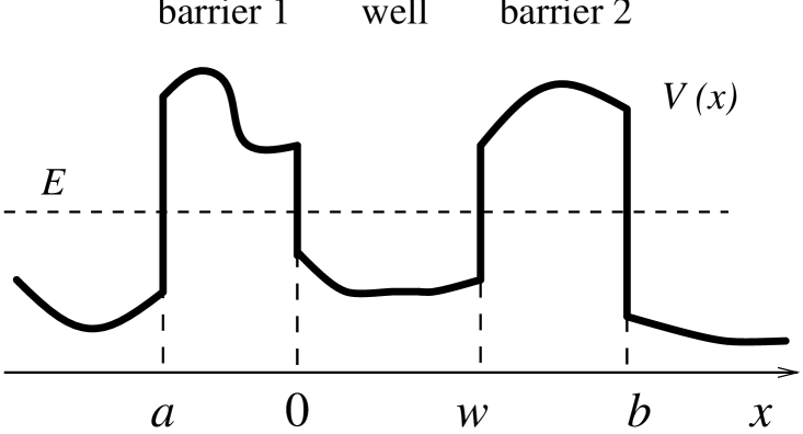
FIG. 1.: The one-dimensional potential $V(x)$ defines the two barriers [$(a,0)$ and $(w,b)$] and the well $(0,w)$.

FIG. 2.: The double barrier structure is split into two regions at $x=x^{\prime}$: $r_{r}(x^{\prime})$ is the reflection coefficient for a plane wave of energy $E$ incident on $V_{r}(x)$ from the left and $r_{l}(x^{\prime})$ is the reflection coeffincient for a plane wave of energy $E$ incident on $V_{l}(x)$ from the right.

REFERENCES

- [1] Fax number: ++39-50-568522; e-mail address: ianna@pimac2.iet.unipi.it
- [2] G. Iannaccone, Phys. Rev. B 51, 4727 (1995).
- [3] L. D. Landau and E. M. Lifshitz, Quantum Mechanics (Non-Relativistic Theory) (Pergamon Press, Oxford, 1977), p. 603.
- [4] T. Weil and B. Vinter, Appl. Phys. Lett. 50, 1281 (1987).
- [5] M. Büttiker, IBM J. Res. Develop. 32, 63 (1988).
- [6] A. D. Stone and P. A. Lee, Phys. Rev. Lett. 54, 1196 (1985).
- [7] M. Jonson and A. Grincwajg, Appl. Phys. Lett. 51, 1729 (1987).
- [8] N. W. Ashcroft and N. D. Mermin, Solid State Physics (Saunders College, Philadelphia, 1976), pp. 9,52,244-246. Relevant characteristic lengths of electron motion are discussed in C. W. J. Beenakker and H. van Houten, in Solid State Physics, vol. 44, H. Ehrenreich and D. Turnbull, eds. (Academic Press, Boston, 1991), pp. 7,19-23,36-49.
- [9] Eq. A4-A12 of Ref. 4 imply that transmission and reflection probabilities do not depend upon energy, i.e., that electrode chemical potentials are close enough that electrons contributing to the net current have energies in a very narrow energy range. Otherwise, the incoherent transmission probability in A12 of Ref. 4 is still valid, provided that we do not include energy relaxation in the extra reservoir and impose on the extra branch that all current contributions at any energy be zero, and not only the net current flow.
- [10] A. Knäbchen, Phys. Rev. B 45, 8542 (1992).
- [11] G. Iannaccone and B. Pellegrini, accepted for publication on Phys. Rev. B.
- [12] A. I. Baz’, Sov. J. Nucl. Phys. 5, 161 (1967).
- [13] D. Sokolovski and L.M. Baskin, Phys. Rev. A 36, 4604 (1987).
- [14] M. Büettiker, Phys. Rev. B 27, 6178 (1983).
- [15] C. R. Leavens and G. C. Aers, Phys. Rev. B 40, 5387 (1989)
- [16] E. H. Hauge and J. A. Støvneng, Rev. Mod. Phys. 61, 197 (1989).
- [17] C. R. Leavens, Solid State Comm. 74, 923 (1990).
- [18] G. Iannaccone and B. Pellegrini, Phys. Rev. B 49, 16548 (1994).
- [19] G. Iannaccone and B. Pellegrini, Phys. Rev. B 50, 14662 (1994).
- [20] R. Landauer and Th. Martin, Rev. Mod. Phys. 66 217 (1994);
- [21] J. R. Barker, S. Brouard, V. Gasparian, G. Iannaccone, A.P. Jauho, C. R. Leavens, J. G. Muga, R. Sala, D. Sokolovski , Phantoms Newsletter 7, 5 (1994).
- [22] J. G. Muga, S. Brouard, and R. Sala, J. Phys: Condens. Matter 4, L579 (1992).
- [23] These points are no more controversial if one adopts Bohm’s interpretation of quantum mechanics; see C. R. Leavens and G. C. Aers, in Scanning Tunneling Microscopy III, edited by R. Wiesendanger and H.-J. Güntherodt, Springer Series in Surface Sciences, Vol. 29 (Springer-Verlag, Berlin Heidelberg, 1993), p. 105.
- [24] P. Erdös and R. C. Herndon, Adv. Phys. 31, 64 (1983).
- [25] B. Riccò and M. Ya. Azbel, Phys. Rev. B 29, 1970 (1984).
- [26] D. K. Ferry, in Physics of Quantum Electron Devices, F. Capasso, ed. (Springer-Verlag, Berlin-Heidelberg, 1990), p. 77.
- [27] H. C. Liu and T. C. L. G. Sollner, Semiconductor and Semimetals, 41, 359 (1994).
- [28] Y. Ando and T. Itoh, J. Appl. Phys. 61, 1497 (1987).
- [29] A. Modinos, G. C. Aers, and B. V. Paranjape, Phys. Rev. B 19, 3996 (1979).
- [30] G. Garcìa Calderón and A. Rubio, Solid State Comm. 71, 237 (1989).