Anisotropic Scaling in Threshold Critical Dynamics of
Driven Directed Lines

Abstract

The dynamical critical behavior of a single directed line driven in a random medium near the depinning threshold is studied both analytically (by renormalization group) and numerically, in the context of a Flux Line in a Type-II superconductor with a bulk current $\vec{J}$. In the absence of transverse fluctuations, the system reduces to recently studied models of interface depinning. In most cases, the presence of transverse fluctuations are found not to influence the critical exponents that describe longitudinal correlations. For a manifold with $d=4-\epsilon$ internal dimensions, longitudinal fluctuations in an isotropic medium are described by a roughness exponent $\zeta_{\parallel}=\epsilon/3$ to all orders in $\epsilon$, and a dynamical exponent $z_{\parallel}=2-2\epsilon/9+O(\epsilon^{2})$. Transverse fluctuations have a distinct and smaller roughness exponent $\zeta_{\perp}=\zeta_{\parallel}-d/2$ for an isotropic medium. Furthermore, their relaxation is much slower, characterized by a dynamical exponent $z_{\perp}=z_{\parallel}+1/\nu$, where $\nu=1/(2-\zeta_{\parallel})$ is the correlation length exponent. The predicted exponents agree well with numerical results for a flux line in three dimensions. As in the case of interface depinning models, anisotropy leads to additional universality classes. A nonzero Hall angle, which has no analogue in the interface models, also affects the critical behavior.

I Introduction and Summary

The study of dynamical critical phenomena associated with the pinning-depinning transition in random media has become a subject of considerable interest in recent years. This is due to the importance of pinning in a wide variety of technologically important phenomena such as flux line (FL) motion in Type-II superconductors, dynamics of interfaces (phase boundaries, invasion fronts, cracks, surface growth, to name a few), and charge-density wave (CDW) transport. These systems are characterized by a rough energy landscape due to the randomness in the medium. At zero temperature there are two distinct “phases”, distinguished by an order parameter (henceforth called velocity) that measures the dynamic response, such as the average velocity for a FL, or current for a CDW. For small driving forces, the system is trapped by one of the many available metastable stationary states, and is “pinned” to the impurities in the medium. Critical behavior emerges as the stationary states disappear, and the system starts moving with a nonzero velocity, when the driving force is increased above a threshold value. Extensive experimental [1], theoretical[2, 3, 4], and simulation[5] work has been done to understand the properties of this transition in CDW systems. There are also numerous studies on the depinning of driven interfaces[6, 7, 8, 9, 10, 11]. A better theoretical understanding of this dynamical phase transition was recently achieved, and critical exponents were calculated through an $\epsilon$-expansion for both CDW systems[3] and driven interfaces[7, 8]. More recently, we performed similar calculations for the depinning of an elastic line in a bulk random medium, like a polymer in a gel network, a FL in a type-II superconductor, or a screw dislocation in a crystal[12]. In this article, we present a detailed report of our study on the dynamical critical behavior associated with the depinning of a FL, and in general on the depinning of directed manifolds in random media, through methods similar to those used for CDWs and interfaces.

Specifically, let us consider the geometry of the FL shown in Fig. 1. The superconductor is subject to a magnetic field $\vec{B}=B{\hat{x}}$ along the $x$-axis, and a bulk supercurrent $\vec{J}=J{\hat{z}}$ along the $z$-axis. A FL is oriented along $\vec{B}$ on the average, but deviates from a straight line due to impurities in the superconductor, which are represented by a potential $V(x,y,z)$. The conformations of the FL are described by $\vec{R}(x,t)=x{\hat{x}}+{\bf r}(x,t)$, where ${\bf r}(x,t)=y(x,t){\hat{y}}+z(x,t){\hat{z}}$ is a two component vector, lying in a plane normal to the magnetic field. The bulk current $\vec{J}$ drives the FL along the $y$-direction through the Lorentz Force $\vec{F}_{L}=\Phi_{0}\vec{J}\times\vec{B}$. ($\Phi_{0}$ is the flux quantum.) If the bulk current is large enough, the FL drifts with an average velocity ${\bf v}$. Due to the chiral nature of the supercurrents around the FL, ${\bf v}$ is in general not along the $y$-direction, but makes an angle $\phi$ with the $y$-axis. This is usually called the Hall angle, and although typically small[13], it can be significant near the depinning transition.

It is more convenient to work with components of ${\bf r}$ that are parallel and perpendicular to ${\bf v}$, i.e.

$${\bf r}(x,t)={r_{\parallel}}(x,t){\bf e_{\parallel}}+{r_{\perp}}(x,t){\bf e_{\perp}},$$ (1)

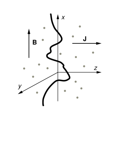
(a)

(b)

FIG. 1.: Geometry of the FL in a medium with impurities: (a) Three-dimensional geometry. (b) A cross section of the medium at fixed $x$. The average drift velocity ${\bf v}=v{\bf e_{\parallel}}$ makes an angle $\phi$ with the $y-$axis.

where the unit vectors ${\bf e_{\parallel}}$ and ${\bf e_{\perp}}$ are rotated by $\phi$ from the $y$- and $z$-axes respectively, as shown in Fig. 1b. In Sec.II we show that, under very general assumptions, the equation of motion for small deviations around a straight line, generalized to $d$-dimesional internal coordinates ${\bf x}\in\Re^{d}$, can be written as

$$\eta\partial_{t}{r_{\parallel}}\! = \!K_{11}\nabla_{\bf x}^{2}{r_{\parallel}}\!+K_{12}\nabla_{\bf x}^{2}{r_{\perp}}\!+F\!+\!\tilde{f_{\parallel}}({\bf x},{\bf r}({\bf x},t)),$$ (3)

$$\eta\partial_{t}{r_{\perp}}\! = \!K_{21}\nabla_{\bf x}^{2}{r_{\parallel}}\!+K_{22}\nabla_{\bf x}^{2}{r_{\perp}}\!+\!\tilde{f_{\perp}}({\bf x},{\bf r}({\bf x},t)),$$ (4)

where $\eta$ is the viscosity the FL and $F=\Phi_{0}J$. The moduli $K_{\alpha\gamma}$ relate the elastic force to the local curvature and are in general nondiagonal for a sample with orientation-dependent core energy, or nonzero Hall angle (cf. Sec. II). The random forces $\tilde{f}_{\alpha}$ that arise from the impurity potential $V$ are taken to have zero mean with correlations

$$\langle\tilde{f}_{\alpha}({\bf x},{\bf r})\tilde{f}_{\gamma}({\bf x}^{\prime},{\bf r}^{\prime})\rangle=\delta^{d}({\bf x}-{\bf x}^{\prime})\tilde{\Delta}_{\alpha\gamma}({\bf r}-{\bf r}^{\prime}),$$ (5)

where $\tilde{\Delta}$ is a function that decays rapidly for large values of its argument. (The indices $\alpha,\gamma,\dots=\{\parallel,\perp\}$.)

Ignoring fluctuations of the FL transverse to the direction of average velocity, i.e. setting ${r_{\perp}}=0$, leads to an interface depinning model studied by Nattermann, Stepanow, Tang, and Leschhorn (NSTL)[7], and by Narayan and Fisher (NF)[8]. Hence, the major difference between Eqs.(1) (henceforth called the “vector depinning model”) and the previously studied “interface model” is the existence of transverse fluctuations, making the position of the line ${\bf r}$ a vector instead of a scalar “height” variable. The effects of such transverse fluctuations for large driving forces and average velocities, when the randomness in the medium can be approximated as uncorrelated in space and time, were shown[14, 15] to create a much richer dynamical phase diagram than the corresponding interface growth model, namely the Kardar-Parisi-Zhang (KPZ) equation[16]. Then, the natural questions to ask are: How do these transverse fluctuations scale near the depinning threshold, and how do they influence the critical dynamics of longitudinal fluctuations?

In order to make these questions more quantifiable, we consider the exponents that characterize the critical behavior near the depinning transition. Let ${\bf F}({\bf v})$ denote the driving force required to move the FL with a velocity ${\bf v}=v{\bf e_{\parallel}}$. For small values of $F=|{\bf F}|$, the line is pinned by the disorder in the medium. There is a threshold force $F_{c}$, such that the line moves with a nonzero average velocity $v$ iff $F>F_{c}$[17]. For $F$ slightly above threshold, we expect the average velocity to scale as

$$v=A(F-F_{c})^{\beta},$$ (6)

where $\beta$ is the velocity exponent and $A$ is a nonuniversal constant. Superposed on the steady advance of the line are rapid “jumps” as portions of the line depin from strong pinning centers. Such jumps are similar to avalanches in other slowly forced systems and have a power-law distribution in size, cut off at a characteristic correlation length $\xi$. On approaching the threshold, $\xi$ diverges as

$$\xi\sim(F-F_{c})^{-\nu},$$ (7)

defining a correlation length exponent $\nu$. At length scales up to $\xi$, the interface is self-affine, with correlations satisfying the dynamic scaling form

$$\langle[{r_{\parallel}}({\bf x},t)-{r_{\parallel}}({\bf 0},0)]^{2}\rangle = |{\bf x}|^{2\zeta_{\parallel}}g_{\parallel}(t/|{\bf x}|^{z_{\parallel}}),$$ (8)

$$\langle[{r_{\perp}}({\bf x},t)-{r_{\perp}}({\bf 0},0)]^{2}\rangle = |{\bf x}|^{2\zeta_{\perp}}g_{\perp}(t/|{\bf x}|^{z_{\perp}}),$$ (9)

where $\zeta_{\alpha}$ and $z_{\alpha}$ are roughness and dynamic exponents, respectively. The scaling functions $g_{\alpha}$ go to a constant as their arguments approach 0; $\zeta_{\parallel}$ and $\zeta_{\perp}$ are the longitudinal and transverse wandering exponents of an instantaneus line profile; $z_{\parallel}$ and $z_{\perp}$ characterize scaling of relaxation times of longitudinal and transverse modes with wave vector through $\tau_{\alpha}(q)\sim q^{-z_{\alpha}}$. Beyond the length scale $\xi$, regions move more or less independently of each other and the system is no longer critical. The behavior of the moving line is described by the exponents calculated earlier[14, 15] for time dependent noise. Ignoring any potential nonlinearities leads to a regular diffusion equation with white noise, for which the roughness and dynamic exponents are $\zeta^{+}_{\parallel}=\zeta^{+}_{\perp}=(2-d)/2,\,z^{+}=2$. In the interface model, transverse fluctuations do not exist, thus, $\zeta_{\perp}$ and $z_{\perp}$ are not defined.

Equations (1) can be analyzed using the formalism of Martin, Siggia, and Rose (MSR)[18]. A renormalization group (RG) treatment of the “interface model”, studied by NSTL[7] and NF[8], indicates an upper critical dimension of $d_{c}=4$, and exponents in $d=4-\epsilon$ dimensions, given to one-loop order as $\zeta=\epsilon/3$ and $z=2-2\epsilon/9$. NSTL obtained this result by directly averaging the MSR generating functional $Z$, and calculating the renormalization of the force-force correlation function $\tilde{\Delta}(r)$. NF, on the other hand, expanded $Z$ around a saddle point solution corresponding to a mean-field approximation[19] to Eqs.(1) which involves temporal force-force correlations $C(vt)$. They point out some of the deficiencies of conventional low-frequency analysis, and suggest that the roughness exponent is equal to $\epsilon/3$ to all orders in perturbation theory. They also show that for two different classes of disordered systems, random-field and random-bond disorder, the zero temperature interface dynamics is essentially the same near threshold. Their argument remains valid for vector depinning, and our results will be applicable to both types of randomness. As we shall demonstrate in Section III, the longitudinal exponents of the “vector” model are identical to those of the depinning interface, and given by

$$\zeta_{\parallel} = \epsilon/3,$$ (10)

$$z_{\parallel} = 2-2\epsilon/9+O(\epsilon^{2}).$$ (11)

Other exponents are determined by exact exponent identities from $\zeta_{\parallel}$ and $z_{\parallel}$ as

$$\nu = \frac{1}{2-\zeta_{\parallel}}=\frac{3}{6-\epsilon},$$ (12)

$$\beta = (z_{\parallel}-\zeta_{\parallel})\nu=1-\epsilon/9+O(\epsilon^{2}).$$ (13)

Following the formalism of NF, we employ a perturbative expansion of the disorder-averaged MSR partition function around a mean-field solution for scalloped impurity potentials[8]. We show that slightly above threshold, transverse fluctuations do not significantly affect the dynamics of longitudinal fluctuations, apart from shifting the threshold force $F_{c}$. Specifically, the exponents and exponent identities given in Eqs. (10–13) for $d<d_{c}$ are also correct for the vector depinning model. However, transverse fluctuations turn out to scale differently, with $\zeta_{\perp}\neq\zeta_{\parallel}$ and $z_{\perp}\neq z_{\parallel}$. In particular, in an isotropic medium with Hall angle $\phi=0$ (Model A in Section II), the renormalization of transverse temporal force-force correlations $C_{\perp}(vt)$ yields

$$\zeta_{\perp}=\zeta_{\parallel}-\frac{d}{2}=-2+\frac{5\epsilon}{6},\\$$ (14)

correct to all orders in $\epsilon$. The transverse dynamic exponent is given by an exact exponent identity:

$$z_{\perp}=z_{\parallel}+\frac{1}{\nu}=4-\frac{5\epsilon}{9}+O(\epsilon^{2}).$$ (15)

These conclusions can also be generalized to more than one transverse direction: the results do not depend on the number of transverse coordinates. For the FL $(\epsilon=3)$, the critical exponents are then predicted to be

$$\begin{array}[]{lll}\zeta_{\parallel}=1,&z_{\parallel}\approx 4/3,&\nu=1,\\ \beta\approx 1/3,&\zeta_{\perp}=1/2,&z_{\perp}\approx 7/3.\end{array}$$ (16)

This implies that in a type II superconductor driven slightly above threshold, flux lines are contained mostly in the plane normal to the current, up to the correlation length scale $\xi$. This may have a noticeable effect on the dynamics of entanglement of flux lines near depinning. These results also rationalize the use of a “planar approximation” in numerical simulations of FL depinning[20].

Another important consideration is the role of anisotropy in the bulk material. It was recently shown that anisotropy leads to new universality classes in interface depinning[21]. We show that this happens as well for FL depinning, in an even richer fashion. The presence of a nonzero Hall angle affects the critical behavior in a manner similar to anisotropy. These issues are discussed in more detail in Section VIII.

The rest of the paper is organized as follows: In Section II, we derive the general form of the equation of motion for a single FL, starting from a reparametrization invariant (RI) descpription of the FL dynamics. In Section III, we first establish the connection of Eqs. (1) to the interface depinning problem for the simple case of an isotropic medium with zero Hall angle. We then examine the linear response of the system to derive the exponent identities (12),(13), and (15), which are later shown to be consistent with a formal RG treatment of the problem in more general circumstances. In Section IV, we present the MSR formalism and expand the generating functional around a self-consistent saddle point solution, given by a mean-field theory. In Section V, we calculate response and connected correlation functions of the mean-field theory, which correspond to the bare propagators and vertex functions in a perturbative expansion. In Section VI, we determine critical exponents through an $\epsilon$-expansion near $d=4$ dimensions, and in Sec. VII we compare these with numerical results obtained by directly integrating the equations of motion. Finally, in Section VIII we discuss the physical significance of these results, the roles of nonlinear terms and anisotropy, and applicability of similar methods to related problems.

II Equations of Motion for a FL

In this section we derive a phenomenological equation that describes the coarse-grained (in space and time) evolution of a single FL in a bulk type-II superconductor. The configuration of the FL at time $t$ is described by ${\vec{R}}(s,t)$, where $s$ is an arbitrary parameter which we shall later equate to the $x-$component of ${\vec{R}}$. The equations of motion are obtained by balancing the “conservative” and “dynamical” forces. Conservative forces are derived from the energy functional and depend only on the instantaneous configuration $\vec{R}(s)$ of the FL. They include the elastic force, random forces due to the impurity potential $V$, and the Lorentz force due to the bulk current. Dynamical forces, on the other hand, depend explicitly on the local velocity of the FL and comprise the dissipative and Magnus forces[22].

For notational simplicity, we set the external magnetic field $\vec{B}$ along the $x$-axis and the the average velocity $\vec{v}$ along ${\bf e_{\parallel}}$, suppressing the possible dependence of parameters on the relative orientation of $\vec{B}$ and ${\bf e_{\parallel}}$ due to anisotropy in the underlying material. Such complications will be taken up later in Sec. VIII. An important consideration is the requirement that the equation of motion be invariant under an arbitrary reparametrization ${\vec{R}}(s)\to{\vec{R}}(s^{\prime})$ of the curve. One such reparametrization invariant quantity is the infinitesimal arclength $dl=ds\sqrt{g}$, where $g\equiv\partial_{s}{\vec{R}}\cdot\partial_{s}{\vec{R}}$ is the metric. The only physically observable motions of the FL are orthogonal to the local unit tangent vector

$\displaystyle{\hat{t}}={1\over\sqrt{g}}\partial_{s}{\vec{R}}.$

Assuming that the FL motion is overdamped, the conservative force $\vec{F}_{T}$, which is derived below, is balanced by dynamical forces that are proportional to the local normal velocity $\vec{v}_{n}={\cal P}\cdot\partial_{t}\vec{R}=\partial_{t}\vec{R}-(\partial_{t}\vec{R}\cdot\hat{t})\hat{t}$. (Here, ${\cal P}_{ij}\equiv\delta_{ij}-\hat{t}_{i}\hat{t}_{j}$ projects any vector onto the local normal plane.) Dynamical forces are not necessarily parallel to $\vec{v}_{n}$: In general, there is an angle $\phi$ (called the Hall angle) between the applied force and the velocity of the FL. Physically, this is due to the Magnus force which is orthogonal to the velocity, and the Hall effect in the normal core of the FL[23]. The equation of motion can then be written as

$$\eta{\cal P}\cdot\left\{\cos\phi\,\partial_{t}{\vec{R}}+\sin\phi(\partial_{t}{\vec{R}})\times{\hat{t}}\right\}={\vec{F}_{T}}.$$ (17)

To determine the conservative force $\vec{F}_{T}$, consider the energy cost associated with a particular coarse-grained configuration ${\vec{R}}(s)$ of the FL in the absence of a bulk current, which is

$$E\left[{\vec{R}}(s)\right]=\int ds\sqrt{g}\left\{\frac{\partial_{s}{\vec{R}}\cdot{\mbox{\boldmath$\sigma$}}\cdot\partial_{s}{\vec{R}}}{g}+V({\vec{R}}(s))\right\}.$$ (18)

In the above equation, the symmetric tensor $\sigma$ gives the core energy per unit length of the FL, and can be nondiagonal for an anisotropic sample. (Anharmonic contributions to the core energy can be ignored in a coarse-grained description and we will systematically keep only the leading order elastic terms.) The restoring force ${\vec{F}}_{B}$ is given by the energy cost of an infinitesimal virtual displacement $\delta{\vec{R}}(s)$. After some rearrangement, we arrive at

$$\delta E = -\int ds\sqrt{g}\,\delta\vec{R}\cdot{\cal P}\cdot\left\{2{\mbox{\boldmath$\sigma$}}\cdot\vec{\kappa}-\left(\hat{t}\cdot{\mbox{\boldmath$\sigma$}}\cdot\hat{t}\right)\vec{\kappa}\phantom{\nabla_{{\vec{R}}}V({\vec{R}})}\right.$$ (20)

$$\left.\qquad\qquad\qquad\qquad\qquad+V({\vec{R}})\vec{\kappa}-\nabla_{{\vec{R}}}V({\vec{R}})\right\}$$

$$\equiv -\int ds\sqrt{g}\,\delta{\vec{R}}\cdot{\vec{F}}_{B},$$ (21)

where $\vec{\kappa}=g^{-1}{\cal P}\cdot\partial_{s}^{2}{\vec{R}}$ is the local curvature vector. To leading order, the random potential $V({\vec{R}})$ that multiplies $\vec{\kappa}$ can be approximated by its spatial average, and eliminated without loss of generality by choosing $\langle V\rangle=0$. ${\vec{f}}=-\nabla_{\vec{R}}V({\vec{R}})$ acts as a random force on each segment of the FL, whose correlations in general satisfy

$$\langle f_{\alpha}({\vec{R}})f_{\gamma}({\vec{R}}^{\prime})\rangle=\Delta_{\alpha\gamma}({\vec{R}}-{\vec{R}}^{\prime}).$$ (22)

For now, we do not restrict the form of $\Delta$, apart from the reasonable expectation that it decays quickly beyond a characteristic impurity size $a$. When a bulk current ${\vec{J}}$ is present, the FL is also subject to a Lorentz force ${\vec{F}}_{L}=\Phi_{0}{\vec{J}}\times{\hat{t}}$, where $\Phi_{0}$ is the flux quantum. Thus, the total conservative force acting on a section of the FL is given as

$${\vec{F}_{T}}={\cal P}\!\cdot\!\left\{\frac{2{\mbox{\boldmath$\sigma$}}\cdot{\cal P}\cdot\partial_{s}^{2}{\vec{R}}-(\hat{t}\cdot{\mbox{\boldmath$\sigma$}}\cdot\hat{t})\partial_{s}^{2}{\vec{R}}}{g}+\Phi_{0}{\vec{J}}\times{\hat{t}}+\vec{f}\right\}.$$ (23)

For an isotropic sample in the extreme type-II limit, the Bardeen-Stephen model gives[23]

$$\sigma_{ij} \approx \delta_{ij}(\Phi_{0}/4\pi\lambda_{s})^{2}\ln(\xi_{s}/\lambda_{s}),$$

$$\eta \approx \Phi_{0}^{2}/(2\pi\xi_{s}^{2}c^{2}\rho_{n}),$$

$$\tan\phi \approx \rho_{n}/\rho_{n}^{H},$$

where $\lambda_{s}$ is the London penetration depth, $\xi_{s}$ is the coherence length, and $\rho_{n},\rho_{n}^{H}$ are normal and Hall resistivities of the non-superconducting core region, respectively. More general expressions for these phenomenological parameters can be derived from a mesoscopic model based on a time-dependent Ginzburg-Landau theory[25].

Equation (17) is highly nonlinear and generalizes those of ref.[26] to the three-dimensional and anisotropic case. We now pick $\{\hat{x},{\bf e_{\parallel}},{\bf e_{\perp}}\}$ as our coordinate axes, and $x$ as the arbitrary parameter $s$, representing the FL as ${\vec{R}}(x,t)=x\hat{x}+{r_{\parallel}}(x,t){\bf e_{\parallel}}+{r_{\perp}}(x,t){\bf e_{\perp}}$. In this representation, $g=1+(\partial_{x}{r_{\parallel}})^{2}+(\partial_{x}{r_{\perp}})^{2}$, $\vec{J}=J_{\parallel}{\bf e_{\parallel}}+J_{\perp}{\bf e_{\perp}}$, $\vec{f}=f_{x}\hat{x}+{f_{\parallel}}{\bf e_{\parallel}}+{f_{\perp}}{\bf e_{\perp}}$, and

$\displaystyle{\mbox{\boldmath$\sigma$}}=\pmatrix{\sigma_{x}&\sigma_{x\parallel}&\sigma_{x\perp}\cr\sigma_{x\parallel}&\sigma_{\parallel}&\sigma_{\times}\cr\sigma_{x\perp}&\sigma_{\times}&\sigma_{\perp}}.$

After some rearrangement, and elimination of higher-order terms coming from the elastic energy of the FL, we obtain the following evolution equations for the components ${r_{\parallel}}$ and ${r_{\perp}}$:

$${\eta\over\cos\phi}\partial_{t}{r_{\parallel}} = [(2\sigma_{\parallel}-\sigma_{x})-2\sigma_{\times}\tan\phi]\partial_{x}^{2}{r_{\parallel}}+[2\sigma_{\times}-(2\sigma_{\perp}-\sigma_{x})\tan\phi]\partial_{x}^{2}{r_{\perp}}$$ (27)

$$\ +{\Phi_{0}\over\sqrt{g}}\left\{J_{\perp}\left[1+(\partial_{x}{r_{\parallel}})^{2}\right]-J_{\parallel}\left[\partial_{x}{r_{\parallel}}\partial_{x}{r_{\perp}}-\tan\phi\sqrt{g}\right]\right\}$$

$$\ +{f_{\parallel}}\left[1+{\tan\phi\over\sqrt{g}}\partial_{x}{r_{\parallel}}\partial_{x}{r_{\perp}}\right]-{f_{\perp}}{\tan\phi\over\sqrt{g}}\left[1+(\partial_{x}{r_{\parallel}})^{2}\right]-f_{x}\left[\partial_{x}{r_{\parallel}}-{\tan\phi\over\sqrt{g}}\partial_{x}{r_{\perp}}\right],$$

$${\eta\over\cos\phi}\partial_{t}{r_{\perp}} = [2\sigma_{\times}+(2\sigma_{\parallel}-\sigma_{x})\tan\phi]\partial_{x}^{2}{r_{\parallel}}+[(2\sigma_{\perp}-\sigma_{x})+\sigma_{\times}\tan\phi]\partial_{x}^{2}{r_{\perp}}$$ (32)

$$\ +{\Phi_{0}\over\sqrt{g}}\left\{J_{\perp}\left[\partial_{x}{r_{\parallel}}\partial_{x}{r_{\perp}}+\tan\phi\sqrt{g}\right]-J_{\parallel}\left[1+(\partial_{x}{r_{\perp}})^{2}\right]\right\}$$

$$\ +{f_{\parallel}}{\tan\phi\over\sqrt{g}}\left[1+(\partial_{x}{r_{\perp}})^{2}\right]+{f_{\perp}}\left[1-{\tan\phi\over\sqrt{g}}\partial_{x}{r_{\parallel}}\partial_{x}{r_{\perp}}\right]-f_{x}\left[\partial_{x}{r_{\perp}}+{\tan\phi\over\sqrt{g}}\partial_{x}{r_{\parallel}}\right].$$

These equations are clearly too complicated for an exhaustive analysis. However, it is possible to perform a gradient expasion of the RHS of Eqs.(II) when the fluctuations around the straight line are small, i.e. $(\partial_{x}{r_{\parallel}})^{2},(\partial_{x}{r_{\perp}})^{2}\ll 1$. In that case, Eqs.(II) simplify to

$${\eta\over\cos\phi}\partial_{t}{r_{\parallel}}\! = \![(2\sigma_{\parallel}-\sigma_{x})-2\sigma_{\times}\tan\phi]\partial_{x}^{2}{r_{\parallel}}+[2\sigma_{\times}-(2\sigma_{\perp}-\sigma_{x})\tan\phi]\partial_{x}^{2}{r_{\perp}}$$ (35)

$$\ +\Phi_{0}\!\left(J_{\perp}+J_{\parallel}\tan\phi\right)\!+\!{f_{\parallel}}\!-\!{f_{\perp}}\tan\phi,\!\!$$

$${\eta\over\cos\phi}\partial_{t}{r_{\perp}} = [2\sigma_{\times}+(2\sigma_{\parallel}-\sigma_{x})\tan\phi]\partial_{x}^{2}{r_{\parallel}}+[(2\sigma_{\perp}-\sigma_{x})+\sigma_{\times}\tan\phi]\partial_{x}^{2}{r_{\perp}}$$ (39)

$$\ +\Phi_{0}\!\left(J_{\perp}\tan\phi-J_{\parallel}\right)\!+\!{f_{\perp}}\!-\!{f_{\parallel}}\tan\phi,$$

neglecting all terms of $O\left((\partial_{x}{r_{\parallel}})^{2},(\partial_{x}{r_{\perp}})^{2}\right)$ or higher.

So far, we have not enforced the condition that ${\bf e_{\parallel}}$ points along the average velocity of the FL. This is satisfied by the self-consistency relation

$$\langle\partial_{t}{r_{\perp}}\rangle=0.$$ (40)

In the small fluctuation limit where Eqs.(II) are valid, this condition is satisfied simply by setting $J_{\parallel}=J_{\perp}\tan\phi$. In order to study the scaling properties of this system in the framework of a field theory, we generalize the FL to a manifold with $d$-dimensional internal coordinates ${\bf x}\in\Re^{d}$. Further rearrangements, and addition of an infinitesimal external force ${\mbox{\boldmath$\varepsilon$}}({\bf x},t)$ in order to study response functions, lead to

$$\eta\partial_{t}{r_{\parallel}}=K_{11}\nabla_{\bf x}^{2}{r_{\parallel}} + K_{12}\nabla_{\bf x}^{2}{r_{\perp}}+F+\tilde{f_{\parallel}}({\bf x},{\bf r}({\bf x},t))+\varepsilon_{1}({\bf x},t),$$ (42)

$$\eta\partial_{t}{r_{\perp}}=K_{21}\nabla_{\bf x}^{2}{r_{\parallel}} + K_{22}\nabla_{\bf x}^{2}{r_{\perp}}+\tilde{f_{\perp}}({\bf x},{\bf r}({\bf x},t))+\varepsilon_{2}({\bf x},t),$$ (43)

where $F=\Phi_{0}\sqrt{J_{\parallel}^{2}+J_{\perp}^{2}}=\Phi_{0}J$, and

$$\pmatrix{K_{11}&K_{12}\cr K_{21}&K_{22}} = \pmatrix{\cos\phi&-\sin\phi\cr\sin\phi&\cos\phi}\pmatrix{2\sigma_{\parallel}-\sigma_{x}&2\sigma_{\times}\cr 2\sigma_{\times}&2\sigma_{\perp}-\sigma_{x}},$$

$$\pmatrix{\tilde{f_{\parallel}}\cr\tilde{f_{\perp}}} = \pmatrix{\cos\phi&-\sin\phi\cr\sin\phi&\cos\phi}\pmatrix{{f_{\parallel}}\cr{f_{\perp}}}.$$

The correlations of the random forces satisfy

$$\langle\tilde{f}_{\alpha}({\bf x},{\bf r})\tilde{f}_{\gamma}({\bf x},{\bf r}^{\prime})\rangle=\delta^{d}({\bf x}-{\bf x}^{\prime})\tilde{\Delta}_{\alpha\gamma}({\bf r}-{\bf r}^{\prime}).$$ (44)

(Note that while both ${\bf r}$ and ${\bf x}$ are represented by bold characters, ${\bf r}$ remains two dimensional, while ${\bf x}$ has been promoted to a $d$-dimensional vector.)

In the special case of an isotropic medium with $\phi=0$, the equations further reduce to

$$\eta\partial_{t}{r_{\parallel}} = K\nabla_{\bf x}^{2}{r_{\parallel}}+F+{f_{\parallel}}({\bf x},{\bf r}({\bf x},t))+\varepsilon_{1}({\bf x},t),$$ (46)

$$\eta\partial_{t}{r_{\perp}} = K\nabla_{\bf x}^{2}{r_{\perp}}+{f_{\perp}}({\bf x},{\bf r}({\bf x},t))+\varepsilon_{2}({\bf x},t),$$ (47)

where the correlations of the random forces satisfy

$$\langle f_{\alpha}({\bf x},{\bf r})f_{\gamma}({\bf x},{\bf r}^{\prime})\rangle=\delta_{\alpha\gamma}\delta^{d}({\bf x}-{\bf x}^{\prime})\Delta(|{\bf r}-{\bf r}^{\prime}|).$$ (48)

We shall henceforth refer to Eqs.(II) as Model A. Anisotropy and/or a nonzero Hall angle changes the scaling properties of the critical region, and we shall refer to this more general case, described by Eqs.(40), as Model B.

III The Vector Depinning Model

In this section, we study some properties of the system described by Eqs.(40) and (II), in detail. Due to statistical translational symmetry in time $t$ and internal coordinates ${\bf x}$, we use the real $({\bf x},t)$ and Fourier $({\bf q},\omega)$ domains interchangeably when dealing with statistical averages.

The vector depinning model differs from the CDW or interface problems due to the presence of transverse fluctuations ${r_{\perp}}({\bf x},t)$. It is sometimes useful to recast the equations such that ${r_{\perp}}$ appears as a function of ${r_{\parallel}}$ rather than $t$. The asymmetry in ${r_{\parallel}}$ and ${r_{\perp}}$ occurs because ${r_{\parallel}}$ almost always moves in the forward direction[24], and therefore is a monotonous function of $t$. Thus, for any particular realization of the random force $f({\bf x},{\bf r})$, there is a unique point ${r_{\perp}}({\bf x},{r_{\parallel}})$ that is visited by the line for given coordinates $({\bf x},{r_{\parallel}})$. The evolution of ${r_{\perp}}({\bf x},{r_{\parallel}})$ can be obtained schematically, by dividing Eq.(40b) by (40a), as

$$\frac{\partial{r_{\perp}}}{\partial{r_{\parallel}}}=\frac{K_{21}\nabla_{\bf x}^{2}{r_{\parallel}}+K_{22}\nabla_{\bf x}^{2}{r_{\perp}}+\tilde{f_{\perp}}}{K_{11}\nabla_{\bf x}^{2}{r_{\parallel}}+K_{12}\nabla_{\bf x}^{2}{r_{\perp}}+\tilde{f_{\parallel}}+F}.$$ (49)

We shall see that in most cases, the scaling properties of ${r_{\perp}}$ in relation to ${r_{\parallel}}$ can be obtained heuristically by inspecting Eq.(49).

A Model A

First of all, we establish the connection between Eq.(II) and the interface depinning model for the special case of an isotropic system with $\phi=0$ (Model A). For a particular realization of randomness ${\bf f}({\bf x},{\bf r})$, Eq.(IIa) can be written as

$$\eta\partial_{t}{r_{\parallel}}=K\nabla_{\bf x}^{2}{r_{\parallel}}+f^{\prime}\left({\bf x},{r_{\parallel}}({\bf x},t)\right)+F+\varepsilon_{1}({\bf x},t),$$ (50)

where $f^{\prime}({\bf x},{r_{\parallel}})={f_{\parallel}}\left({\bf x},{r_{\parallel}},{r_{\perp}}({\bf x},{r_{\parallel}})\right)$ and ${r_{\perp}}({\bf x},{r_{\parallel}})$ is determined by Eq.(49). It is quite plausible that, after averaging over all ${\bf f}$, the correlations in $f^{\prime}$ will also be short-ranged, albeit different from those of ${\bf f}$, since the dissipative dynamics will avoid maxima of the random potential, effectively reducing the average forces. In that case, the equation reduces exactly to the model studied by NSTL and NF. Thus, the scaling of longitudinal fluctuations of the FL near threshold will not change upon taking into account transverse components, and the exponent relations (10–13) hold for Model A as well. We expect this argument to hold even for Model B [Eqs.(40)] as long as $\nabla_{\bf x}^{2}{r_{\perp}}\ll\nabla_{\bf x}^{2}{r_{\parallel}}$, or when $\zeta_{\perp}<\zeta_{\parallel}$.

For the interface model, it is possible to show that $v(F)$ is a single valued function using the “no passing rule” of Middleton[4]. The rule states that no interface (or CDW) can overtake another, if initially every point on the first interface is behind the second one. This rule does not apply to the vector model: It is in principle possible to have coexistence of moving and stationery FLs, allowing for the possibility of a discontinuous (multi-valued) ${\bf v}({\bf F})$. However, since a moving line samples an arbitrarily large region in the medium, it is plausible that the velocity self-averages at long times, resulting in a single valued ${\bf v}({\bf F})$ (i.e., no hysteresis). However, finite-size systems do suffer from such hysteresis which adversely affects numerical simulations of the model. These issues are further discussed in Sec.VII.

Several exponent identities can be deduced from the form of the linear response,

$$\chi_{\alpha\gamma}({\bf q},\omega)=\left<\frac{\partial r_{\alpha}({\bf q},\omega)}{\partial\varepsilon_{\gamma}({\bf q},\omega)}\right>,$$ (51)

in the $({\bf q},\omega)\to({\bf 0},0)$ limit. Due to the statistical symmetry of Eqs.(II) under the transformation ${r_{\perp}}\to-{r_{\perp}}$, the linear response is diagonal. Let us first set $\omega=0$ and examine the static response: An additional static force ${\mbox{\boldmath$\varepsilon$}}({\bf q})$ with zero spatial average (no ${\bf q}=0$ component) can be exactly compensated by the coordinate change

$\displaystyle{\bf r}^{\prime}_{\alpha}({\bf q},t)={\bf r}_{\alpha}({\bf q},t)+(Kq^{2})^{-1}\varepsilon_{\alpha}({\bf q}).$

The distribution of ${\bf f}$ does not change in the primed coordinates. Thus, the static linear response has the form

$$\chi_{\alpha\gamma}({\bf q},\omega=0)=\delta_{\alpha\gamma}\frac{1}{Kq^{2}}.$$ (52)

Since $\varepsilon_{\parallel}$ scales like the applied force, the form of the linear response at the correlation length $\xi$ gives the exponent identity

$$\zeta_{\parallel}+1/\nu=2.$$ (53)

Considering the transverse linear response seems to imply $\zeta_{\perp}=\zeta_{\parallel}$. However, as will be shown below, the static part of the transverse linear response becomes irrelevant at the critical RG fixed point, since $z_{\perp}>z_{\parallel}$. This is consistent with the expectation that the dynamics is responsible for the distinction between longitudinal and transverse modes.

Why are the relaxational dynamics different in the two fluctuation directions near depinning? The answer can be traced to a simple symmetry argument, which requires ${\bf F}$ and ${\bf v}$ to remain parallel, i.e.

$${\bf F}({\bf v})=F(v){\hat{v}},$$ (54)

where ${\hat{v}}={\bf v}/v$, and $F$ is some (scalar) function which depends on only the magnitude $v$, of velocity. For small deviations around ${\bf v}=v{\bf e_{\parallel}}$, we thus obtain (see Fig. 2)

$$\frac{\partial F_{\parallel}}{\partial v_{\parallel}} = \frac{dF}{dv},$$ (55)

$$\frac{\partial F_{\perp}}{\partial v_{\perp}} = \frac{F}{v}.$$ (56)

FIG. 2.: A graphical demonstration of Eqs.(55- 56). When a longitudinal force is applied, the direction is not changed and all changes are in the magnitude $F(v)$. For a transverse force, $F$ does not change to linear order in $dF_{\perp}$, but ${\bf v}$ changes direction to remain parallel to ${\bf F}$.

These two derivatives clearly scale differently in the $v\to 0$ limit, which causes a separation of relaxation time scales, as shown below.

Now consider the response to a spatially uniform (${\bf q}={\bf 0}$), but time-dependent, external force ${\mbox{\boldmath$\varepsilon$}}(t)$. The leading term in the dynamic response is intricately connected to ${\bf v}({\bf F})$: When a slowly varying uniform external force ${\mbox{\boldmath$\varepsilon$}}(t)$ is applied, the FL responds as if the instantaneous external force ${\bf F}+{\mbox{\boldmath$\varepsilon$}}$ is a constant, i.e. it moves with the average velocity

$$\langle\partial_{t}r_{\alpha}\rangle=v_{\alpha}({\bf F}+{\mbox{\boldmath$\varepsilon$}})\approx v_{\alpha}({\bf F})+\frac{\partial v_{\alpha}}{\partial F_{\gamma}}\varepsilon_{\gamma}.$$ (57)

Therefore, near the depinning transition,

$$\chi_{\parallel}({\bf q}=0,\omega) \simeq \frac{1}{-i\omega(dF/dv)+O(\omega^{2})},$$ (58)

$$\chi_{\perp}({\bf q}=0,\omega) \simeq \frac{1}{-i\omega(F_{c}/v)+O(\omega^{2})}.$$ (59)

Eq.(52) can be combined with the above to yield a Taylor expansion of the inverse linear response around $({\bf q},\omega)=({\bf 0},0)$ that reads

$$\chi_{\parallel}^{-1}({\bf q},\omega) \simeq Kq^{2}-i\omega(dF/dv)+{\rm h.o.t.},$$ (60)

$$\chi_{\perp}^{-1}({\bf q},\omega) \simeq Kq^{2}-i\omega(F_{c}/v)+{\rm h.o.t.}$$ (61)

The zero of $\chi^{-1}$ in the complex $\omega-$plane for a given value of the wavevector ${\bf q}$ gives the relaxation time of the corresponding mode. Thus, the relaxation times of fluctuations with wavelength $\xi$ are

$$\tau_{\parallel}(q=\xi^{-1}) \sim \left(q^{2}\frac{dv}{dF}\right)^{-1}\sim\xi^{2+(\beta-1)/\nu}\sim\xi^{z_{\parallel}},$$ (62)

$$\tau_{\perp}(q=\xi^{-1}) \sim \left(q^{2}\frac{v}{F_{c}}\right)^{-1}\sim\xi^{2+\beta/\nu}\sim\xi^{z_{\perp}},$$ (63)

which in turn yield

$$\beta = 1+(z_{\parallel}-2)\nu,$$ (64)

$$z_{\perp} = z_{\parallel}+1/\nu.$$ (65)

Thus, $z_{\perp}>z_{\parallel}$ as noted earlier. This difference arises entirely from the different scaling properties of $dv/dF$ $[\sim(F-F_{c})^{\beta-1}]$ and $v/F$ $[\sim(F-F_{c})^{\beta}]$ near the depinning transition, as noted earlier.

B Model B

A similar linear response analysis can be made for the more general case of Model B. The leading contributions to the static and dynamic part of the inverse linear response are given by

$$\chi^{-1}_{\alpha\gamma}({\bf q},\omega=0) = K_{\alpha\gamma}q^{2},$$ (66)

$$\chi^{-1}_{\alpha\gamma}({\bf q}={\bf 0},\omega) = -i\omega(\partial v_{\alpha}/\partial F_{\gamma})^{-1}.$$ (67)

The relation between the external force and the drift velocity can in general be written as

$${\bf F}({\bf v})=F(v,\theta)\left[\cos\phi(v,\theta){\hat{v}}+\sin\phi(v,\theta){\hat{x}}\times{\hat{v}}\right].$$ (68)

Both $F$ and $\phi$ in general depend on the orientation of ${\hat{v}}$, parametrized by an angle $\theta$ in the $yz$-plane. Then, for small deviations around ${\bf v}=v{\bf e_{\parallel}}$,

$$\pmatrix{dF_{\parallel}\cr\cr dF_{\perp}\cr}=\pmatrix{A_{11}&-\frac{1}{v}A_{12}\cr\cr A_{21}&\frac{1}{v}A_{22}\cr}\pmatrix{dv_{\parallel}\cr\cr dv_{\perp}\cr},$$ (69)

where

$$A_{11} = \partial_{v}(F\cos\phi),$$

$$A_{21} = \partial_{v}(F\sin\phi),$$

$$A_{12} = F\sin\phi-\partial_{\theta}(F\cos\phi),$$

$$A_{22} = F\cos\phi+\partial_{\theta}(F\sin\phi).$$

The scaling of diagonal elements in the linear response are the same as in Model A. Therefore, exponent identities (64-65) hold in the more general case of Model B as well.

IV MSR Formalism

We use the formalism of MSR[18] to compute response and correlation functions for the dynamical system described by Eqs. (40). After some rearranging, we obtain

$$\eta\frac{\partial r_{\alpha}({\bf x},t)}{\partial t}=\int{d^{d}\!x\,}^{\prime}\,J_{\alpha\gamma}({\bf x}-{\bf x}^{\prime})r_{\gamma}({\bf x}^{\prime},t)$$ (71)

$$-r_{\alpha}({\bf x},t)+\tilde{f}_{\alpha}\left({\bf x},{\bf r}({\bf x},t)\right)+F_{\alpha}+\varepsilon_{\alpha}({\bf x},t),$$

where the tensor J is given by its Fourier transform as $J_{\alpha\gamma}({\bf q})=\delta_{\alpha\gamma}-K_{\alpha\gamma}q^{2}$. Introducing an auxiliary field ${\bf\hat{r}}({\bf x},t)$, the generating functional $Z$ is given by

$$Z=\int{[d{\bf r}][d{\bf\hat{r}}]{\cal J}[{\bf r}]\exp(S)},$$ (72)

where

$$S=i\int{d^{d}\!x\,}{dt\,}{\hat{r}}_{\alpha}({\bf x},t)\left\{\eta\partial_{t}r_{\gamma}-K_{\alpha\gamma}\nabla_{\bf x}^{2}r_{\gamma}\right.$$ (74)

$$\left.-F_{\alpha}-\tilde{f}_{\alpha}\left({\bf x},{\bf r}({\bf x},t)\right)-\varepsilon_{\alpha}({\bf x},t)\right\}.$$

Clearly, this coarse-grained continuum picture of the system breaks down at length scales shorter than the core radius of the FL. Therefore, there is a natural cutoff $\Lambda$ in q-space for the functional integrals in Eq. (72). $Z$ can be used to generate response and correlation functions of ${\bf r}$, since integrating over ${\bf\hat{r}}$ gives delta functions that impose the solution to the equation of motion (71). The Jacobian ${\cal J}[{\bf r}]$ fixes the renormalization of $Z$ such that the delta functions integrate to unity, and will be suppressed henceforth. Since $Z=1$ independent of the realization of randomness, response and correlation functions can also be generated using the disorder-averaged generating function $\overline{Z}=\int{[d{\bf r}][d{\bf\hat{r}}]\langle\exp(S)\rangle}$. For example, the two-point correlation function is given by

$\displaystyle\langle r_{\alpha}({\bf x},t)r_{\gamma}({\bf x}^{\prime},t^{\prime})\rangle=\int{[d{\bf r}][d{\bf\hat{r}}]r_{\alpha}({\bf x},t)r_{\gamma}({\bf x}^{\prime},t^{\prime})\langle\exp(S)\rangle},$

and the linear response is

$\displaystyle\left<\frac{\delta r_{\alpha}({\bf x},t)}{\delta\varepsilon_{\gamma}({\bf x}^{\prime},t^{\prime})}\right>=-i\int{[d{\bf r}][d{\bf\hat{r}}]r_{\alpha}({\bf x},t){\hat{r}}_{\gamma}({\bf x}^{\prime},t^{\prime})\langle\exp(S)\rangle}.$

In order proceed, we discretize in ${\bf x}$-space: ${\bf r}({\bf x},t)\to{\bf r}_{i}(t)$. Introducing two conjugate fields ${\bf R}_{i}(t),{\bf\hat{R}}_{i}(t)$, $\overline{Z}$ can be rewritten as

$${\overline{Z}} = \int[d{\bf R}][d{\bf\hat{R}}]\exp(\tilde{S}),$$ (75)

$$\tilde{S} = \sum_{j}\ln{\overline{Z}_{j}}\left({\bf R}_{j},{\bf\hat{R}}_{j}\right)$$ (77)

$$\quad-i\int{dt\,}\sum_{i,j}{\bf\hat{R}}_{i}(t)\cdot{\bf J}^{-1}_{ij}\cdot{\bf R}_{j}(t),$$

where ${\overline{Z}_{j}}\left({\bf R}_{j},{\bf\hat{R}}_{j}\right)$ is given by

$${\overline{Z}_{j}} = \int{[d{\bf r}_{j}][d{\bf\hat{r}}_{j}]\left<\exp\int{dt\,}\left[i{\bf\hat{R}}_{j}(t)\cdot{\bf r}_{j}(t)\right.\right.}$$ (80)

$$\quad+i{\bf\hat{r}}_{j}(t)\cdot\left\{\eta\partial_{t}{\bf r}_{j}(t)-{\bf R}_{j}(t)\right.$$

$$\left.{\phantom{\int}}\left.{\phantom{\bf\hat{R}}}\left.+{\bf r}_{j}(t)-\tilde{\bf f}_{j}\left({\bf r}_{j}(t)\right)-{\bf F}-{\mbox{\boldmath$\varepsilon$}}_{j}(t)\right\}\right]\right>.$$

Note that this factorization of the disorder-dependent part of the action to local functionals ${\overline{Z}_{j}}$ is possible only if the random forces $\tilde{\bf f}_{j}$ are independent at each site $j$, as assumed in Eq. (5). ${\overline{Z}_{j}}$ can be evaluated by an expansion around the saddle-point approximation. The integrand of the exponential is a maximum when, for each $j$,

$$-\sum_{i}{\bf J}_{ij}^{-1}\cdot{\bf\hat{R}}_{i}^{0}-\left<{\bf\hat{r}}_{j}\right>_{\rm MF}={\bf 0},$$

$$-\sum_{i}{\bf J}_{ij}^{-1}\cdot{\bf R}_{i}^{0}+\left<{\bf r}_{j}\right>_{\rm MF}={\bf 0},$$

which has a solution ${\bf\hat{R}}^{0}_{j}={\bf 0},\;{\bf R}^{0}_{j}={\bf v}t$ for all $j$. Here, v is determined self-consistently as a function of F by requiring $\left<{\bf r}_{j}\right>_{\rm MF}={\bf v}t$, where averages $(\left<\dots\right>_{\rm MF})$ are generated from ${\overline{Z}_{j}}$ evaluated at the saddle point, which is identical for each $j$:

$$Z_{\rm MF}=\int[d{\bf r}_{j}][d{\bf\hat{r}}_{j}]\left<\exp i\int dt\;{\bf\hat{r}}_{j}(t)\right.$$ (82)

$$\left.{\phantom{\int}}\cdot\left\{{\eta\partial_{t}{\bf r}_{j}}(t)-{\bf v}t+{\bf r}_{j}(t)-\tilde{\bf f}_{j}\left({\bf r}_{j}(t)\right)-{\bf F}-{\mbox{\boldmath$\varepsilon$}}_{j}(t)\right\}\right>.$$

$Z_{\rm MF}$ can be identified as the MRS generating function for a mean-field (MF) approximation to Eq. (71), obtained by setting $J_{\alpha\gamma}({\bf x}-{\bf x}^{\prime})=\delta_{\alpha\gamma}N^{-1}$, where $N=\int d^{d}x$. (The first term in the RHS of (71) is then self-consistently equal to $\langle{\bf r}\rangle_{\rm MF}={\bf v}t$.) Redefining the field variables as ${\bf R}\to{\bf R}+{\bf v}t,\,i{\bf\hat{R}}\to{\bf\hat{R}}$ (for notational simplicity), the expansion for $\ln{\overline{Z}_{j}}\left({\bf R}_{j},{\bf\hat{R}}_{j}\right)$ is given by

$$\ln{\overline{Z}_{j}}\left({\bf R}_{j},{\bf\hat{R}}_{j}\right)=\sum_{\{m_{\alpha},n_{\alpha}\}=0}^{\infty}\left(\prod_{\alpha}\frac{1}{m_{\alpha}!n_{\alpha}!}\right)$$ (85)

$$\times\int\prod_{\alpha}\left\{\prod_{s_{\alpha}=1}^{m_{\alpha}}dt_{\alpha s_{\alpha}}{\hat{R}}_{j\alpha}(t_{\alpha s_{\alpha}})\prod_{s_{\alpha}^{\prime}=1}^{n_{\alpha}}dt_{\alpha s_{\alpha}^{\prime}}^{\prime}R_{j\alpha}(t_{\alpha s_{\alpha}^{\prime}}^{\prime})\right\}$$

$$\qquad\qquad\qquad\qquad\times{\cal V}_{\{m_{\alpha},n_{\alpha}\}}\left(\{t_{\alpha s_{\alpha}}\};\{t_{\alpha s_{\alpha}^{\prime}}^{\prime}\}\right).$$

The vertex functions ${\cal V}$ are obtained by evaluating derivatives of $\ln{\overline{Z}_{j}}$ with respect to the fields at the saddle point, and are given precisely by connected correlation and response functions of the MF system decribed by Eq. (82):

$${\cal V}_{\{m_{\alpha},n_{\alpha}\}}\left(\{t_{\alpha s_{\alpha}}\};\{t_{\alpha s_{\alpha}^{\prime}}^{\prime}\}\right)$$ (86)

$$= \left[\prod_{\alpha}\prod_{s_{\alpha}^{\prime}=1}^{n_{\alpha}}\frac{\partial}{\partial\varepsilon_{j\alpha}(t_{\alpha s_{\alpha}^{\prime}}^{\prime})}\right]\left<\prod_{\alpha}\prod_{s_{\alpha}=1}^{m_{\alpha}}r_{j\alpha}(t_{\alpha s_{\alpha}})\right>_{{\rm MF},c}.$$ (87)

Thus, once the mean-field system is solved, correlation functions of ${\bf R},{\bf\hat{R}}$ can be studied through a momentum space RG treatment to obtain the scaling exponents of the fields in the long-time, large wavelength (hydrodynamic) limit. ${\bf R}$ and ${\bf\hat{R}}$ are like coarse-grained forms of the original fields ${\bf r}$ and ${\bf\hat{r}}$ since all correlation functions of ${\bf r},{\bf\hat{r}}$ are equal to corresponding correlation functions of ${\bf R},{\bf\hat{R}}$ in the hydrodynamic limit[3]. Therefore, it is sufficient to find the scaling behavior of ${\bf R},{\bf\hat{R}}$ to deduce the desired critical exponents.

V Mean Field Theory

In this section, we calculate response and correlation functions of the local system described by $Z_{\rm MF}$, which gives the vertex functions in the diagrammatic expansion of $\tilde{S}$. We will only need to calculate the leading terms as higher order vertices will turn out to be irrelevant in the critical region. Due to the averaging, $Z_{\rm MF}$ is identical at all sites $j$, and it is sufficient to examine a single point. Setting $\overline{\bf r}(t)\equiv{\bf r}_{j}(t)-{\bf v}t$, and ${\mbox{\boldmath$\varepsilon$}}(t)\equiv{\mbox{\boldmath$\varepsilon$}}_{j}(t)$, the equation of motion becomes

FIG. 3.: (a) The effective potential $V_{\rm eff}$. The random part (not shown) superimposed on the paraboloid slides with velocity $-{\bf v}$. (b) A cross section of $V_{\rm eff}$. The particle stays in a local minimum $P$ for a time of $O(v^{-1})$, after which the minimum disappears and the particle finds another local minimum $P^{\prime}$ within a finite time. Time averages are dominated by the slow portion of the motion as $v\to 0$.

$$\eta\left(\frac{d\overline{r}_{\alpha}}{dt}+v_{\alpha}\right)=-\overline{r}_{\alpha}+F_{\alpha}+\tilde{f}_{\alpha}\left({\bf v}t+\overline{\bf r}(t)\right)+\varepsilon_{\alpha}(t).$$ (88)

${\bf F}$ is determined as a function of ${\bf v}$ self-consistently by requiring that $\langle\overline{\bf r}\rangle_{\rm MF}={\bf 0}$. The scaling behavior of ${\bf F}_{\rm MF}({\bf v})$ near threshold can be determined from the following argument: For $v\ll\eta^{-1}F$, the particle follows a local minimum $P$ of the effective potential

$\displaystyle V_{\bf eff}(\overline{\bf r},t)=V\left({\bf x},{\bf v}t+\overline{\bf r}(t)\right)+\frac{|\overline{\bf r}(t)|^{2}}{2}-{\bf F}\cdot\overline{\bf r}(t).$

A representative snapshot of $V_{\bf eff}$, which consists of a paraboloid centered at $\overline{\bf r}={\bf F}$ with a superimposed random potential, is shown in Fig. 3. The position of the local minimum $P$ shifts with a velocity of $O(v)$ as time progresses. Eventually, $P$ disappears at a saddle point as it is pushed up the sides of the hyperparaboloid. At this moment, the particle quickly moves to a new local minimum $P^{\prime}$, after which it starts following the slow motion of $P^{\prime}$, as shown in Fig. 3. For scalloped random potentials with discontinuous derivatives at the saddle points, the particle starts moving with a velocity of $O(1)$ (i.e., independent of $v$ as $v\to 0$) as soon as $P$ disappears, and reaches the vicinity of $P^{\prime}$ in $O(1)$ time, giving the result $\beta_{\rm MF}=1$. (In contrast, for smooth potentials, there is a $v$-dependent acceleration time just after $P$ disappears, which contributes to the critical dynamics and gives $\beta_{\rm MF}=3/2.$[2, 4].) We have also numerically integrated Eq. (88) (for Model A) to verify that $\beta_{\rm MF}=1$.

Next, we proceed to compute vertex functions ${\cal V}_{\{m_{\alpha},n_{\alpha}\}}\left(\{t_{\alpha s_{\alpha}}\};\{t_{\alpha s_{\alpha}^{\prime}}^{\prime}\}\right)$ in the perturbative expansion of $\tilde{S}$, which correspond to response and connected correlation functions of the MF theory, in increasing order in the field variables ${\bf R},{\bf\hat{R}}$. From now on, we set $m=m_{\parallel}+m_{\perp}$, and $n=n_{\parallel}+n_{\perp}$.

A Average position (m=1, n=0)

By construction $\left<\overline{\bf r}\right>_{\rm MF}=0$, but we prefer to expand around the true ${\bf F}({\bf v})$ instead of the mean-field value of the force ${\bf F}_{\rm MF}({\bf v})$. Since the effect of an additional uniform static force ${\bf F}-{\bf F}_{\rm MF}({\bf v})$ can be fully counteracted by a shift in $\overline{\bf r}$, this does not affect connected correlation or response functions. Thus, the only effect of this shift is to produce an additional term $\sum_{i}[{\bf F}-{\bf F}_{\rm MF}({\bf v})]\cdot{\bf\hat{R}}_{i}$ in $\tilde{S}$, which only has a $q=0$ component and does not directly enter the renormalization of higher order terms.

B Linear Response (m=1, n=1)

The linear response is given by the rank 2 tensor,

$\displaystyle{\tilde{\chi}}_{\alpha\gamma}(t-t^{\prime})=\left<\frac{\delta\overline{r}_{\alpha}(t)}{\delta\varepsilon_{\gamma}(t^{\prime})}\right>_{\rm MF}.$

We are only interested in the low-frequency form of the Fourier transformed linear response ${\tilde{\mbox{\boldmath$\chi$}}}(\omega)$, i.e. when $\varepsilon$ is slowly varying in time. In this case, we can write ${\mbox{\boldmath$\varepsilon$}}(t)\approx{\mbox{\boldmath$\varepsilon$}}_{0}+{\mbox{\boldmath$\varepsilon$}}_{1}t$, neglecting terms proportional to $\ddot{\mbox{\boldmath$\varepsilon$}}$. To find the response $\overline{\bf r}_{\mbox{\boldmath$\varepsilon$}}(t)$, let us define

$\displaystyle\overline{\bf r}_{\mbox{\boldmath$\varepsilon$}}^{\prime}(t)=\overline{\bf r}_{\mbox{\boldmath$\varepsilon$}}(t)-{\mbox{\boldmath$\varepsilon$}}_{0}-{\mbox{\boldmath$\varepsilon$}}_{1}t-{\bf F}_{\rm MF}({\bf v})+{\bf F}_{\rm MF}({\bf v}+{\mbox{\boldmath$\varepsilon$}}_{1}).$

Taking a time derivative and using Eq.(88), we obtain

$$\eta(\dot{\overline{\bf r}}^{\prime}_{\mbox{\boldmath$\varepsilon$}}+{\bf v}+{\mbox{\boldmath$\varepsilon$}}_{1})=-\overline{\bf r}^{\prime}_{\mbox{\boldmath$\varepsilon$}} + {\bf F}_{\rm MF}({\bf v}+{\mbox{\boldmath$\varepsilon$}}_{1})$$ (89)

$$+ \tilde{\bf f}(({\bf v}+{\mbox{\boldmath$\varepsilon$}}_{1})t+\overline{\bf r}_{\mbox{\boldmath$\varepsilon$}}^{\prime}-{\bf F}_{\mbox{\boldmath$\varepsilon$}}),$$ (90)

where ${\bf F}_{\mbox{\boldmath$\varepsilon$}}={\bf F}_{\rm MF}({\bf v}+{\mbox{\boldmath$\varepsilon$}}_{1})-{\bf F}_{\rm MF}({\bf v})-{\mbox{\boldmath$\varepsilon$}}_{0}$. But now, $\left<\overline{\bf r}^{\prime}_{\mbox{\boldmath$\varepsilon$}}\right>={\bf 0}$ by definition of ${\bf F}_{\rm MF}$. (The random force $\tilde{\bf f}$ is evaluated at points shifted by a constant amount ${\bf F}_{\mbox{\boldmath$\varepsilon$}}$, but this has no significance upon averaging over randomness.) This gives

$$\langle\overline{\bf r}_{\mbox{\boldmath$\varepsilon$}}(t)\rangle={\mbox{\boldmath$\varepsilon$}}(t)+{\bf F}_{\rm MF}({\bf v})-{\bf F}_{\rm MF}\left({\bf v}+\dot{\mbox{\boldmath$\varepsilon$}}(t)\right)+O(\ddot{\mbox{\boldmath$\varepsilon$}}).$$ (91)

Expanding ${\bf F}_{\rm MF}({\bf v}+\dot{\mbox{\boldmath$\varepsilon$}})$ for small $\dot{\mbox{\boldmath$\varepsilon$}}$, we obtain

$${\tilde{\chi}}_{\alpha\gamma}(\omega)=\delta_{\alpha\gamma}+i\omega\left[\frac{\partial F_{{\rm MF}\alpha}({\bf v})}{\partial v_{\gamma}}\right]_{{\bf v}=v{\bf e_{\parallel}}}+O(\omega^{2}).$$ (92)

Since $\beta_{\rm MF}=1$, the linear response tensor will have the form

$$\tilde{\mbox{\boldmath$\chi$}}(\omega)={\bf 1}+i\omega\pmatrix{A_{11}&-\frac{1}{v}A_{12}\cr\cr A_{21}&\frac{1}{v}A_{22}\cr},$$ (93)

where $A_{\alpha\gamma}$ approach constants as $v\to 0$ (cf. Eq.(69)). For Model A, $\tilde{\mbox{\boldmath$\chi$}}(\omega)$ is diagonal due to symmetry, and $A_{12}=A_{21}=0$.

C Nonlinear response (m=1, n$>$1)

Assuming that ${\bf F}_{\rm MF}({\bf v})$ has a Taylor expansion around ${\bf v}=v{\bf e_{\parallel}}$ for $v>0$, we can expand the RHS of Eq. (91) to obtain the nonlinear response of the model. The leading term in the low-frequency limit is proportional to $\omega^{n}$, and it is straightforward to show that the contribution of these terms to $\tilde{S}$ is

$$-\frac{1}{n_{\parallel}!n_{\perp}!}\int{d^{d}\!x\,} {dt\,} \left[\frac{\partial^{n}F_{\alpha}({\bf v})}{\partial^{n_{\parallel}}v_{\parallel}\partial^{n_{\perp}}v_{\perp}}\right]_{{\bf v}=v{\bf e_{\parallel}}}$$ (95)

$$\times{\hat{R}}_{\alpha}({\bf x},t)(\partial_{t}R_{\parallel})^{n_{\parallel}}(\partial_{t}R_{\perp})^{n_{\perp}}.$$

These terms are irrelevant at the RG fixed point, as we shall show later.

D Two-point Correlation Functions (m=2, n$\geq$0)

At low velocities, the particle spends most of the time near a local minimum, jumping abruptly to the next one when this minimum disappears. Therefore, the time scale associated with the correlation functions is given by the temporal separation between two consecutive jumps, which scales as $1/v$. In the $v\to 0$ limit, the correlation functions depend on $t$ only through the rescaled time variable $u\equiv vt$, since the positions of successive minima near threshold are determined by energetic considerations, and do not depend on $v$. (The correlation functions may also depend on the drift direction ${\hat{v}}$. We shall suppress this dependence for notational brevity.) Let us define

$$\left<\overline{r}_{\alpha}(t)\overline{r}_{\gamma}(t^{\prime})\right>_{{\rm MF},c}\equiv C_{\alpha\gamma}\left(v(t-t^{\prime})\right).$$ (96)

Since successive positions of the local minima are uncorrelated, we expect that $C_{\alpha\gamma}(u)$ decay quickly as a function of $u\equiv vt$ for $|u|>1$. By definition,

$$C_{\parallel}(u) \equiv C_{11}(u)=C_{11}(-u),$$

$$C_{\perp}(u) \equiv C_{22}(u)=C_{22}(-u),$$

$${1\over 2}C_{\times}(u) \equiv C_{12}(u)=C_{21}(-u).$$

As a result of the abrupt jumps from one minimum to another, $C_{\alpha\gamma}(vt)$ have a discontinuous derivative at the origin, rounded at a scale of $O(v)$. In Model A, $C_{\times}(u)=0$ due to symmetry.

The only other important terms in the effective action $\tilde{S}$ involve the series $m=2,n=n_{\parallel}>0,n_{\perp}=0$. All vertex functions associated with this series are given by the response of connected correlation functions to longitudinal forces. These response functions are intimately related to the two-point correlation functions $C_{\alpha\gamma}(u)$ by the following argument: Static forces only change linear response, and do not affect connected correlation functions. For a slowly varying external force $\varepsilon(t){\bf e_{\parallel}}$, however, the system will respond as if the instantaneus velocity is $(v+\dot{\varepsilon}){\bf e_{\parallel}}$. Neglecting terms proportional to $\ddot{\varepsilon}$,

$$\left[\left<\overline{r}_{\alpha}(t)\overline{r}_{\gamma}(t^{\prime})\right>_{{\rm MF},c}\right]_{\varepsilon} = C_{\alpha\gamma}\left((v+\dot{\varepsilon})(t-t^{\prime})\right)+O(\ddot{\varepsilon})$$

$$\approx C_{\alpha\gamma}\left(v(t-t^{\prime})+\varepsilon(t)-\varepsilon(t^{\prime})\right).$$

Now, Taylor expanding $C_{\alpha\gamma}$ around $v(t-t^{\prime})$ and taking successive functional derivatives with respect to $\varepsilon$, we finally obtain the contribution of this series to $\tilde{S}$ as

$${\cal U}=\hbox to0.0pt{$\displaystyle\sum_{n=1}^{\infty}\frac{1}{2!n!}\int{d^{d}\!x\,}{dt\,}dt^{\prime}\,{\hat{R}}_{\alpha}({\bf x},t){\hat{R}}_{\gamma}({\bf x},t^{\prime})$\hss}\quad$$ (98)

$$\qquad\times U_{\alpha\gamma,n}\left(v(t-t^{\prime})\right)\left[R_{\parallel}({\bf x},t)-R_{\parallel}({\bf x},t^{\prime})\right]^{n},$$

where $U_{\alpha\gamma,n}(u)$ is the $n$th derivative of $C_{\alpha\gamma}(u)$.

The vertices with $m=2,n_{\perp}>0$ and $m>3$ are all irrelevant, as shown in the next section.

VI Scaling and RG

The terms in $\tilde{S}$ that are up to second order in the fields are

$${\tilde{S}}_{0} = -\int{dt\,}{d^{d}\!x\,}[{\bf F}-{\bf F}_{\rm MF}({\bf v})]\cdot{\bf\hat{R}}({\bf x},t)$$ (100)

$$\ -\frac{1}{2}\int\limits_{{\bf q},\omega}\left[\matrix{{\bf\hat{R}}(-{\bf q},-\omega)\cr\cr{\bf R}(-{\bf q},-\omega)\cr}\right]^{\rm T}\!\!\!\cdot\!\left[\matrix{-{\bf C}(\omega)&{\bf J}^{-1}({\bf q})-\tilde{\mbox{\boldmath$\chi$}}(\omega)\cr\cr{\bf J}^{-1}(-{\bf q})-\tilde{\mbox{\boldmath$\chi$}}(-\omega)&{\bf 0}\cr}\right]\!\cdot\!\left[\matrix{{\bf\hat{R}}({\bf q},\omega)\cr\cr{\bf R}({\bf q},\omega)}\right],$$

where $J^{-1}_{\alpha\gamma}({\bf q})=\left(\delta_{\alpha\gamma}-K_{\alpha\gamma}q^{2}\right)^{-1}\approx\delta_{\alpha\gamma}+K_{\alpha\gamma}q^{2}$ for small $q$. For notational brevity, we use $\int_{{\bf q},\omega}$ to denote $\int{{d^{d}q\over(2\pi)^{d}}\,}{{d\omega\over 2\pi}\,}$. Using Eq.(93), the quadratic form in the action can be written as

$$-{1\over 2}\int\limits_{{\bf q},\omega}\left[\matrix{{\hat{R}}_{\parallel}(-{\bf q},-\omega)\cr{\hat{R}}_{\perp}(-{\bf q},-\omega)\cr R_{\parallel}(-{\bf q},-\omega)\cr{1\over v}R_{\perp}(-{\bf q},-\omega)}\right]^{\rm T}\cdot{\cal Q}({\bf q},\omega)\cdot\left[\matrix{{\hat{R}}_{\parallel}({\bf q},\omega)\cr{\hat{R}}_{\perp}({\bf q},\omega)\cr R_{\parallel}({\bf q},\omega)\cr{1\over v}R_{\perp}({\bf q},\omega)}\right],$$ (101)

where

$\displaystyle{\cal Q}({\bf q},\omega)=\left[\matrix{-C_{\parallel}(\omega)&-{1\over 2}C_{\times}(\omega)&K_{11}q^{2}-i\omega A_{11}&vK_{12}q^{2}+i\omega A_{12}\cr\cr-{1\over 2}C_{\times}(-\omega)&-C_{\perp}(\omega)&K_{21}q^{2}-i\omega A_{21}&vK_{22}q^{2}-i\omega A_{22}\cr\cr K_{11}q^{2}+i\omega A_{11}&K_{21}q^{2}+i\omega A_{21}&0&0\cr\cr vK_{12}q^{2}-i\omega A_{12}&vK_{22}q^{2}+i\omega A_{22}&0&0\cr}\right].$

Neglecting all higher order terms in the action, we arrive at a Gaussian theory, in which different Fourier modes are decoupled, and which can be solved by inverting the matrix in Eq.(101). (See Appendix A.) The quadratic action (100) remains invariant under the scale transformation

$$\begin{array}[]{ll}{\bf x}\rightarrow b{\bf x},&t\rightarrow b^{2}t,\cr\\ R_{\parallel}\rightarrow b^{2-d/2}{R_{\parallel}},&R_{\perp}\rightarrow b^{2-d}{R_{\perp}},\cr\\ {\hat{R}}_{\parallel}\rightarrow b^{-2-d/2}{{\hat{R}}_{\parallel}},&{\hat{R}}_{\perp}\rightarrow b^{-2-d/2}{{\hat{R}}_{\perp}},\cr\\ v\rightarrow b^{-d/2}v,&F-F_{\rm MF}\rightarrow b^{-d/2}(F-F_{\rm MF}),\end{array}$$ (102)

except for terms proportional to $K_{12}$ and $K_{22}$ which vanish at the depinning transition as $v\to 0^{+}$. For $d>4$, all higher order terms in $\tilde{S}$ decay away upon rescaling, and we recover an asymptotically quadratic theory with critical exponents $\beta=1,\,z_{\parallel}=2,\,\nu=2/d,\,\zeta_{\parallel}=(4-d)/2,\,\zeta_{\perp}=2-d$. The remaining exponent, $z_{\perp}$, can be found by comparing the static and dynamic parts of the transverse linear response. This gives $z_{\perp}=2+d/2=z_{\parallel}+1/\nu$, as shown previously by the exponent identity (15). The exponents related to longitudinal fluctuations, not surprisingly, are identical to corresponding exponents in the interface problem[8]. However, we have also calculated new exponents characterizing transverse fluctuations. We see that even the simple Gaussian theory exhibits anisotropic exponents.

At $d=d_{c}=4$ dimensions, the scaling dimension of $R_{\parallel}$ changes sign and we cannot neglect its higher powers anymore. Simple dimensional analysis indicates that the only higher order terms in $\tilde{S}$ which become marginal at $d=d_{c}$ involve vertex functions $U_{\alpha\gamma,n}$, given in Eq.(98). This series can be summed up over $n$, together with the $n=0$ term $C_{\alpha\gamma}$ included in the Gaussian theory, to yield

$$\frac{1}{2}\int {d^{d}\!x\,} {dt\,}dt^{\prime}{\hat{R}}_{\alpha}({\bf x},t){\hat{R}}_{\gamma}({\bf x},t^{\prime})$$ (104)

$$\times C_{\alpha\gamma}\left(v(t-t^{\prime})+R_{\parallel}({\bf x},t)-R_{\parallel}({\bf x},t^{\prime})\right).$$

All higher order terms in $\tilde{S}$ are formally irrelevant since they involve additional powers of ${\hat{R}}_{\parallel}$, ${\hat{R}}_{\perp}$, or $R_{\perp}$, whose scaling exponents are less than zero.

For $d<d_{c}$, the vertex functions $U_{\alpha\gamma,n}$ become more and more relevant for increasing $n$ under the rescaling (102), and the fixed point moves away from the Gaussian theory. In $d=4-\epsilon$ dimensions, we look for new fixed points with different scaling properties:

$$\begin{array}[]{ll}{\bf x}\rightarrow b{\bf x},&t\rightarrow b^{z_{\parallel}}t,\cr\\ R_{\parallel}\rightarrow b^{\zeta_{\parallel}}{R_{\parallel}},&R_{\perp}\rightarrow b^{\zeta_{\perp}}{R_{\perp}},\cr\\ {\hat{R}}_{\parallel}\rightarrow b^{\theta_{\parallel}-d}{{\hat{R}}_{\parallel}},&{\hat{R}}_{\perp}\rightarrow b^{\theta_{\perp}-d}{{\hat{R}}_{\perp}},\cr\\ F-F_{\rm MF}\rightarrow b^{-1/\nu}(F-F_{\rm MF}),&{\bf v}\rightarrow b^{-\beta/\nu}{\bf v}.\end{array}$$ (105)

To calculate the new exponents to first order in $\epsilon$, we employ a one-loop momentum shell RG scheme, treating all non-Gaussian terms in the action (i.e. $\cal U$ in Eq.(98)), as a perturbation. Perturbative calculations proceed by expanding $\langle e^{\cal U}\rangle_{0}$, where $\langle\cdots\rangle_{0}$ denotes averaging with respect to the Gaussian action $\tilde{S}_{0}$, in powers of ${\cal U}$. A renormalization transformation is then constructed as follows: (1) Perform the averages only over short wavelength fluctuations ${\bf\hat{R}}^{>},{\bf R}^{>}$ with wavenumbers $\Lambda/b<|{\bf q}|<\Lambda$, where $b=e^{\delta\ell}$. The resulting coarse grained action is perturbatively given by

$${\tilde{S}^{<}}={\tilde{S}_{0}^{<}}+\langle{\cal U}\rangle^{>}_{0}+{1\over 2}\langle{\cal U}^{2}\rangle^{>}_{0,c}+O({\cal U}^{3}).$$ (106)

(2) Apply the rescaling transformations given in (105), bringing back the short-distance cutoff $\Lambda$ to its original value. (3) The exponents are then determined from the fixed points associated with the RG flows of the the action. Since Models A and B are characterized by distinct fixed points, we shall discuss them separately.

A Model A

In the low-frequency, small-wavevector limit, the effective action for Model A is

$$\tilde{S}^{(A)} = -\int{dt\,}{d^{d}\!x\,}[F-F_{\rm MF}(v)]{\hat{R}}_{\parallel}({\bf x},t)$$ (110)

$$\quad-\int\limits_{{\bf q},\omega}\left\{{\hat{R}}_{\parallel}(-{\bf q},-\omega)R_{\parallel}({\bf q},\omega)(Kq^{2}-i\omega A_{11})+{\hat{R}}_{\perp}(-{\bf q},-\omega)R_{\perp}({\bf q},\omega)(Kq^{2}-i\omega A_{22}/v)\right\}$$

$$\quad+\frac{1}{2}\int{d^{d}\!x\,}{dt\,}{dt\,}^{\prime}{\hat{R}}_{\parallel}({\bf x},t){\hat{R}}_{\parallel}({\bf x},t^{\prime})C_{\parallel}\left(v(t-t^{\prime})+R_{\parallel}({\bf x},t)-R_{\parallel}({\bf x},t^{\prime})\right)$$

$$\quad+\frac{1}{2}\int{d^{d}\!x\,}{dt\,}{dt\,}^{\prime}{\hat{R}}_{\perp}({\bf x},t){\hat{R}}_{\perp}({\bf x},t^{\prime})C_{\perp}\left(v(t-t^{\prime})+R_{\parallel}({\bf x},t)-R_{\parallel}({\bf x},t^{\prime})\right).$$

The Gaussian part has the correlation functions,

$$\langle{\hat{R}}_{\parallel}(-{\bf q},-\omega)R_{\parallel}({\bf q},\omega)\rangle_{0} = \frac{1}{Kq^{2}-i\omega A_{11}},$$ (112)

$$\langle{\hat{R}}_{\perp}(-{\bf q},-\omega)R_{\perp}({\bf q},\omega)\rangle_{0} = \frac{1}{Kq^{2}-i\omega A_{22}/v},$$ (113)

$$\langle R_{\parallel}(-{\bf q},-\omega)R_{\parallel}({\bf q},\omega)\rangle_{0} = \frac{C_{\parallel}(\omega)}{K^{2}q^{4}+(\omega A_{11})^{2}},$$ (114)

$$\langle R_{\perp}(-{\bf q},-\omega)R_{\perp}({\bf q},\omega)\rangle_{0} = \frac{C_{\perp}(\omega)}{K^{2}q^{4}+(\omega A_{22}/v)^{2}}.$$ (115)

The vertex functions $U_{\alpha\gamma,n}=0$ for $\alpha\neq\gamma$, and these terms are not generated by the RG transformation. The renormalization of remaining vertex functions $U_{\parallel,n}$, and $U_{\perp,n}$ for $n>0$ can be recast into a functional renormalization of $C_{\parallel}(vt)$ and $C_{\perp}(vt)$, provided that $vt$ and $R_{\parallel}$ scale in the same way, i.e. $\zeta_{\parallel}=z_{\parallel}-\beta/\nu$. This relation can be independently obtained from Eqs. (53) and (64), derived in Sec. III from more general (and nonperturbative) arguments. The renormalized vertex functions are then obtained from successive derivatives of $C(vt)$ as

$$U_{\alpha,n}(u)=C^{(n)}_{\alpha}(u).$$ (116)

This ensures that the form of Eq.(110) is retained under renormalization, albeit with renormalized parameters. Eqs. (114) and (115) suggest that $C_{\alpha}(vt)$ may be interpreted as temporal correlation functions of an effective force generated by the quenched disorder.

The renormalization of some terms in Eq.(110) do not get any contribution from the momentum shell averaging step, giving rise to additional exponent relations that are correct to all orders in the $\epsilon$ expansion. The first relation is due to the fact that $F$ never appears explicitly in any of the contractions or higher order vertex functions. Thus, the renormalization of the term proportional to $F-F_{{\rm MF}}$ can be written as

$$\frac{\partial(F-F_{{\rm MF}})}{\partial\ell}=(z_{\parallel}+\theta_{\parallel})(F-F_{{\rm MF}})+{\rm constant},$$ (117)

where “constant” refers to an expression that does not involve $F$. This RG flow equation can be rewritten as

$$\frac{\partial(F-F_{c})}{\partial\ell}=(z_{\parallel}+\theta_{\parallel})(F-F_{c}),$$ (118)

with a suitable choice of $F_{c}$. Hence, higher order corrections may shift the threshold force, but do not influence the scaling of $F-F_{c}$. This implies that

$$z_{\parallel}+\theta_{\parallel}-1/\nu=0.$$ (119)

Furthermore, there are no contractions that contribute to the renormalization of $K$ or $A_{22}$. Thus,

$$\theta_{\parallel}+z_{\parallel}+\zeta_{\parallel}-2 = 0,$$ (120)

$$\theta_{\perp}+\zeta_{\perp}+\beta/\nu = 0,$$ (121)

respectively. As a result, all critical exponents are determined in terms of $\zeta_{\parallel}$, $\zeta_{\perp}$ and $z_{\parallel}$. These exponents can be computed by constructing RG flow equations for the remaining parameters.

1 Renormalization of  $C_{\alpha}$

After performing the momentum shell integration and rescaling, details of which are given in Appendix B, we arrive at the recursion relations for the renormalized functions $C_{\alpha}(u)$:

$$\frac{\partial C_{\parallel}(u)}{\partial\ell} = [\epsilon+2\theta_{\parallel}+2(z_{\parallel}-2)]C_{\parallel}(u)+\zeta_{\parallel}uC^{\prime}_{\parallel}(u)$$ (122)

$$- {K_{d}}\left\{[C^{\prime}_{\parallel}(u)]^{2}+[C_{\parallel}(u)-C_{\parallel}(0)]C^{\prime\prime}_{\parallel}(u)\right\},$$ (123)

$$\frac{\partial C_{\perp}(u)}{\partial\ell} = [\epsilon+2\theta_{\perp}+2(z_{\parallel}-2)]C_{\perp}(u)$$ (124)

$$+ \zeta_{\parallel}u\,C^{\prime}_{\perp}(u)-{K_{d}}\left\{[C_{\parallel}(u)-C_{\parallel}(0)]C^{\prime\prime}_{\perp}(u)\right\}.$$ (125)

The constant $K_{d}\equiv S_{d}\Lambda^{d-4}/[(2\pi)^{d}K^{2}]$, where $S_{d}$ is the total solid angle in $d$-dimensions. Primes denote derivatives with respect to $u$. Terms proportional to $uC^{\prime}_{\alpha}(u)$ arise from the rescaling of $u$. We look for fixed-point solutions $C^{*}_{\alpha}(u)$ that decay to 0 when $|u|$ is large, since they are related to correlation functions of the system, which are expected to vanish for large time differences.

Not surprisingly, the functional recursion relation for $C_{\parallel}(u)$ is identical to the one obtained in Ref. [8]. In fact, all higher loop corrections are identical as well. This is in excellent harmony with the argument presented in Sec. III, and allows us to use the results of NF. Setting $\partial C^{*}_{\parallel}/\partial\ell=0$, and integrating Eq. (122) from $u=-\infty$ to $\infty$, we get

$$[\epsilon+2\theta_{\parallel}+2(z_{\parallel}-2)-\zeta_{\parallel}]\int\limits_{-\infty}^{\infty}C^{*}_{\parallel}(u)\,du=0.$$ (126)

Provided that the RG flows go to a fixed-point solution with $\int C^{*}\neq 0$, this implies that $\zeta_{\parallel}=\epsilon-2[2-(z_{\parallel}+\theta_{\parallel})]$. The mean-field correlation function satisfies this integral condition for both random-field and random-bond disorder, since $C$ is essentially insentitive to the value of the random potential between consecutive local minima $P$, where the line moves quickly. There are other fixed points with $\int C^{*}=0$, but they are irrelevant for our discussion. Thus, from Eqs. (53) and (119), we obtain

$$\zeta_{\parallel} = \epsilon/3,$$ (127)

$$\nu = \frac{3}{6-\epsilon}.$$ (128)

NF prove that these results are correct to all orders in $\epsilon$, by showing that the contributions to the renormalization of $C_{\parallel}(u)$ from higher-order terms is a complete derivative with respect to $u$. Upon integration over $u$, such higher order terms do not alter Eq.(126), leaving the exponents unchanged.

Using $\zeta_{\parallel}=\epsilon/3$, an implicit solution for $C^{*}_{\parallel}(u)$ is obtained as

$\displaystyle C^{*}_{\parallel}(u)-C^{*}_{\parallel}(0)-C^{*}_{\parallel}(0)\ln\left(\frac{C^{*}_{\parallel}(u)}{C^{*}_{\parallel}(0)}\right)={C^{*}(0)\over 2}\left(\frac{u}{u_{0}}\right)^{2},$

where $u_{0}\equiv\sqrt{3K_{d}C^{*}(0)/\epsilon}$. $C_{\parallel}^{*}(0)$ is arbitrary, and can be changed by a rescaling of the fields $R_{\parallel}$. Expanding the logarithm for small $u$, we see that there is a kink at the origin, as

$$\frac{C^{*}_{\parallel}(u)}{C^{*}_{\parallel}(0)}=\left[1-\frac{|u|}{u_{0}}+\frac{1}{3}\left(\frac{u}{u_{0}}\right)^{2}\right]+O(|u/u_{0}|^{3}).$$ (129)

For $|u|\gg u_{0}$, the fixed point solution behaves like a Gaussian, and

$\displaystyle C^{*}_{\parallel}(u)\approx C_{\parallel}^{*}(0)\exp\left[-{u^{2}\over 2u_{0}^{2}}\right].$

We next examine the fixed-point solution $C^{*}_{\perp}(u)$, which is the new element of our computation. Setting $\partial C^{*}_{\perp}/\partial\ell=0$ and looking at the limit $u\to 0^{+}$, we get (assuming that $C^{*}_{\perp}(0^{+})\neq 0$)

$$[\epsilon+2\theta_{\perp}+2(z_{\parallel}-2)]C^{*}_{\perp}(0^{+})=0.$$ (130)

Combined with Eqs.(53), (64), and (121), this result implies

$$\zeta_{\perp}=\zeta_{\parallel}-\frac{d}{2}=-2+\frac{5\epsilon}{6}.$$ (131)

In Appendix C, we show that this result is in fact correct to all orders in $\epsilon$ since there are no contributions to $C^{*}_{\perp}(0^{+})$ from momentum-shell integration. The fixed point solution (for $u>0$) satisfies the equation

$$\frac{d}{du}\ln|C_{\perp}^{*^{\prime}}(u)|=\frac{u}{u_{0}^{2}}\left[\frac{C^{*}_{\parallel}(u)}{C^{*}_{\parallel}(0)}-1\right]^{-1}.$$ (132)

Upon integrating twice, Eq. (132) leads to

$$C^{*}_{\perp}(u)=-{C^{*^{\prime}}_{\perp}(0^{+})}\int\limits_{u}^{\infty}du^{\prime}\,\exp\left\{-\frac{1}{u_{0}^{2}}\int\limits_{0^{+}}^{u^{\prime}}du^{\prime\prime}\,\frac{u^{\prime\prime}}{1-\left[C^{*}_{\parallel}(u^{\prime\prime})/C^{*}_{\parallel}(0)\right]}\right\},$$ (133)

where $C^{*^{\prime}}_{\perp}(0^{+})$ is arbitrary in the same sense as $C^{*}_{\parallel}(0)$. For $|u|\gg u_{0}$, Eq.(132) gives

$$C^{*}_{\perp}(u)\approx C\frac{u_{0}^{2}}{u}\exp\left[-{u^{2}\over 2u_{0}^{2}}\right],$$ (134)

where $C$ is a constant related to $C_{\perp}^{*^{\prime}}(0^{+})$. The numerical solution for the fixed point functions $C_{\alpha}^{*}(u)$ are shown in Fig. 4. The qualitative features of $C^{*}_{\parallel}$ and $C^{*}_{\perp}$ are similar: both have a discontinuous derivative at the origin, and decay as a Gaussian for large values of $|u|$. However, note that their scaling dimensions differ by $\zeta_{\parallel}$.

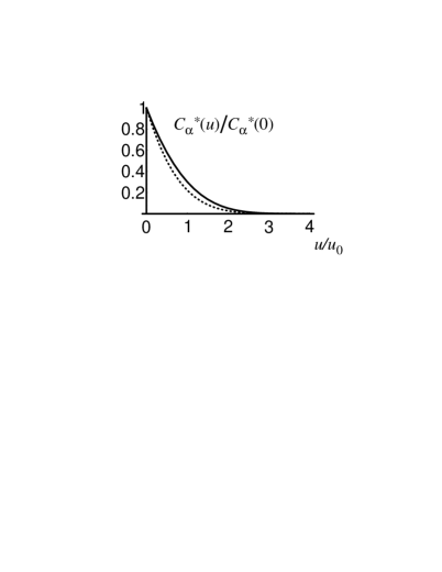
FIG. 4.: Fixed point functions $C^{*}_{\parallel}(u)$ (solid line) and $C^{*}_{\perp}(u)$ (dotted line), normalized to yield 1 at the origin. Their values for $u<0$ (not shown) are found from $C_{\alpha}^{*}(u)=C_{\alpha}^{*}(-u)$.

The exponent $\zeta_{\parallel}=\epsilon/3$ can also be obtained by naive dimensional arguments: In dimensions $d>4$, the random force can be expanded as ${f_{\parallel}}({\bf x},{r_{\parallel}},{r_{\perp}})={f_{\parallel}}({\bf x},0,0)+O({r_{\parallel}},{r_{\perp}})$. Since both ${r_{\parallel}}$ and ${r_{\perp}}$ have negative scaling dimensions $(\zeta_{\parallel},\zeta_{\perp}<0)$, the correction terms can be ignored. The random force scales as $b^{-d/2}$ under a scaling ${\bf x}\to b{\bf x}$, leading to the Gaussian roughness of $\zeta_{\parallel}=2-d/2$. A similar scaling argument applied to Eq.(49) leads to $\zeta_{\perp}=\zeta_{\parallel}-d/2=2-d$. For $d<4$, the scaling dimension of ${r_{\parallel}}$ is positive, and higher powers of ${r_{\parallel}}$ in an expansion of ${f_{\parallel}}({\bf x},{r_{\parallel}},{r_{\perp}})$ are more relevant. It is then reasonable to assume that in this case the statistical properties of ${f_{\parallel}}$ at large ${r_{\parallel}}$ are crucial. If uncorrelated at large separation, ${f_{\parallel}}({\bf x},{r_{\parallel}},0)$ scales as $b^{-(d+\zeta_{\parallel})/2}$. When equated to $b^{\zeta_{\parallel}-2}$ for the scaling of $\nabla_{\bf x}^{2}{r_{\parallel}}$, this leads to $\zeta_{\parallel}=\epsilon/3$ in agreement with the RG treatment. Essentially, the statement regarding the non-renormalization of $\int du\,C_{\parallel}(u)$ justifies the above “naive” scaling. However, a similar reasoning from Eq.(49) would have concluded $\zeta_{\perp}-\zeta_{\parallel}=-(d+\zeta_{\parallel})/2$, in disagreement with Eq.(131). In this case, $\int du\,C_{\perp}(u)$ is renormalized, but $C_{\perp}(0)$ is not; suggesting that despite the presence of relevant higher order powers in the expansion of ${f_{\perp}}({\bf x},{r_{\parallel}},{r_{\perp}})$ around ${\bf r}={\bf 0}$, the scaling properties are still controlled by ${f_{\perp}}({\bf x},0,0)$. We have no physical motivation for this rather curious conclusion.

2 Propagator Renormalization

The only one remaining exponent is $z_{\parallel}$, which can be obtained by examining the renormalization of $A_{11}$. One-loop contributions arise from the $n=2$ term in $\langle{\cal U}\rangle_{0}^{>}$, which is

$$\frac{1}{4}\int d^{d}x\int\limits_{-\infty}^{\infty} dt \int\limits_{-\infty}^{\infty}dt^{\prime}{\hat{R}}_{\parallel}({\bf x},t){\hat{R}}_{\parallel}({\bf x},t^{\prime})$$

$$\times[R_{\parallel}({\bf x},t)-R_{\parallel}({\bf x},t^{\prime})]^{2}C^{\prime\prime}_{\parallel}\left(v(t-t^{\prime})\right).$$

Replacing $[R_{\parallel}({\bf x},t^{\prime})]^{2}$ with $[R_{\parallel}({\bf x},t)]^{2}$ does not change the integral. Thus, upon further manipulation, this term in the action can be written as

$$\int d^{d}x\int\limits_{-\infty}^{\infty} dt \int\limits_{-\infty}^{t}dt^{\prime}{\hat{R}}_{\parallel}({\bf x},t){\hat{R}}_{\parallel}({\bf x},t^{\prime})R_{\parallel}({\bf x},t)$$

$$\times[R_{\parallel}({\bf x},t)-R_{\parallel}({\bf x},t^{\prime})]C^{\prime\prime}_{\parallel}\left(v(t-t^{\prime})\right).$$

Since a contraction forces $t$ and $t^{\prime}$ to be within $O(1)$ of each other, and we are only interested in the first time derivative, we can substitute $R_{\parallel}({\bf x},t)-R_{\parallel}({\bf x},t^{\prime})\approx(t-t^{\prime})\partial_{t}R_{\parallel}({\bf x},t)$. Now, contracting ${\hat{R}}_{\parallel}({\bf x},t^{\prime})$ with $R_{\parallel}({\bf x},t)$ and integrating over the momentum shell, we obtain a contribution to $A_{11}$ equal to

$$-\delta\ell\frac{S_{d}\Lambda^{d}}{(2\pi)^{d}A_{11}}\int\limits_{0}^{\infty}d\tilde{t}\,\tilde{t}\,e^{-K\Lambda^{2}\tilde{t}/A_{11}}C^{\prime\prime}_{\parallel}(v\tilde{t}\,).$$ (135)

The minus sign comes from the opposite overall signs of $m=1$ and $m=2$ terms in Eq. (110). For $v\to 0$, we can set the argument of $C^{\prime\prime}_{\parallel}$ to zero. However, this causes a problem: $C^{\prime\prime}_{\parallel}$ has a term proportional to $\delta(vt)$ in the low-frequency analysis, this term diverges as $1/v$ for $vt\to 0$. This apparent divergence cannot be avoided within the low-frequency analysis we have used so far. The propagator is sensitive to high-frequency behavior of the vertex functions. Careful analysis of the high frequency structure of $C^{\prime\prime}_{\parallel}$ shows that the terms that contribute to the diverging part of $C^{\prime\prime}_{\parallel}(0)$ do not enter the renormalization of the propagator. (See Appendix D.) This is essentially due to the causal nature of the response: Perturbations right after a jump do not influence the motion before the jump. The correct way to avoid these divergent terms within the low-frequency analysis is to use $C^{\prime\prime}_{\parallel}(0^{+})$ instead of $C^{\prime\prime}_{\parallel}(0)$. Near the fixed point, this can be calculated to $O(\epsilon)$ from Eq. (129) as $C^{*^{\prime\prime}}_{\parallel}(0^{+})=2\epsilon/(9K_{d})$, resulting in

$\displaystyle A_{11}^{<}=A_{11}-\delta\ell A_{11}K_{d}C^{*^{\prime\prime}}_{\parallel}(0^{+})=A_{11}[1-\delta\ell(2\epsilon/9)].$

Finally, after performing the rescaling, we obtain the recursion relation

$$\frac{\partial A_{11}}{\partial\ell}=A_{11}[\theta_{\parallel}+\zeta_{\parallel}-2\epsilon/9],$$ (136)

which yields

$$z_{\parallel}=2-2\epsilon/9+O(\epsilon^{2}).$$ (137)

B Model B

The presence of off-diagonal terms in the action changes the critical scaling properties of Model B. The nonzero contractions that appear in the momentum shell integration in this case are (cf. Appendix A)

$$\langle{\hat{R}}_{\parallel}(-{\bf q},-\omega)R_{\parallel}({\bf q},\omega)\rangle_{0} = \frac{1}{K_{\parallel}q^{2}-i\omega\rho_{\parallel}},$$ (139)

$$\langle{\hat{R}}_{\perp}(-{\bf q},-\omega)R_{\parallel}({\bf q},\omega)\rangle_{0} = \frac{\kappa}{K_{\parallel}q^{2}-i\omega\rho_{\parallel}},$$ (140)

$$\langle R_{\parallel}(-{\bf q},-\omega)R_{\parallel}({\bf q},\omega)\rangle_{0} = \frac{{\tilde{C}}(\omega)}{K_{\parallel}^{2}q^{4}+\omega^{2}\rho_{\parallel}^{2}},$$ (141)

where

$$\kappa \equiv A_{12}/A_{22},$$

$$K_{\parallel} \equiv K_{11}+\kappa K_{21},$$

$$\rho_{\parallel} \equiv A_{11}+\kappa A_{21},$$

$${\tilde{C}}(\omega) \equiv C_{\parallel}(\omega)+\kappa{\rm Re}[C_{\times}(\omega)]+\kappa^{2}C_{\perp}(\omega).$$

In addition to the nonrenormalization relations (119-121), the nonrenormalization of $K_{21}$ or $A_{12}$ dictates that

$$\theta_{\parallel}=\theta_{\perp}.$$ (142)

This immediately implies the exponent identity

$$\zeta_{\perp}=\zeta_{\parallel}-1/\nu.$$ (143)

The naive scaling argument based on Eq.(49) gives an equivalent result when the scaling dimension of $\partial{r_{\perp}}/\partial{r_{\parallel}}$ ($\zeta_{\perp}-\zeta_{\parallel}$) is equated to the scaling dimension of ${f_{\perp}}({\bf x},{r_{\parallel}},0)$ [$-(d+\zeta_{\parallel})/2$]. The naive argument works this time, since $\int du\,C_{\perp}(u)$ remains finite at the fixed point (see below).

Under this rescaling, $\kappa$ and $K_{\parallel}$ remain unrenormalized, and the renormalizations of $\rho_{\parallel}$ and $\tilde{C}$ determine the remaining exponents $\zeta_{\parallel}$ and $z_{\parallel}$. The recursion relations of vertex functions $C_{\alpha}$ are more complicated, but there is a relatively simple fixed point solution with

$$\tilde{C}^{*}(u)=4C^{*}_{\parallel}(u)=2\kappa C^{*}_{\times}(u)=4\kappa^{2}C^{*}_{\perp}(u).$$ (144)

Furthermore, $\tilde{C}(u)$ satisfies a recursion relation identical to that of $C_{\parallel}(u)$ given in Eq.(122). This result once more shows that longitudinal fluctuations, whose correlations are given by Eq.(141), are not altered by the introduction of transverse fluctuations even in the more general case of Model B.

The renormalization of $\rho_{\parallel}$ also gives results very similar to that of Model A, with the substitutions $C_{\parallel}^{\prime\prime}\to{\tilde{C}}^{\prime\prime}$ and $A_{11}\to\rho_{\parallel}$. Thus, the RG analysis gives the same exponents $\zeta_{\parallel}=\epsilon/3$ and $z_{\parallel}=2-2\epsilon/9+O(\epsilon^{2})$. Further details appear in Appendix E.

If the Hall Angle $\phi$ is sufficiently small, the FL can not distinguish between zero and nonzero angles. Therefore, the effective roughness and dynamic exponents at small length and time scales should be given by the Model A fixed point. Note that $\kappa=\tan\phi$ in an isotropic system with nonzero Hall angle (cf. Eq.(69)), and $\kappa$ is in general strongly related to the macroscopic Hall angle. Thus, $\kappa\ll 1$ when the system is almost Model A-like, and its nonrenormalization determines the cross-over behavior to the Model B fixed point: Under renormalization with Model A exponents, the system remains near the Model A fixed point until the ratio $C_{\perp}/C_{\parallel}$ increases to $O(\kappa^{-2})$, as the Model B fixed point is approached. Isotropic effective exponents appear in this crossover regime. The length scale $\xi_{\times}$ at which the behavior crosses over to the Model B is roughly given by

$\displaystyle\phi\approx\xi_{\times}^{\zeta_{\perp}-\zeta_{\parallel}},$

(with Model A exponents for $\zeta_{\alpha}$), i.e. the anisotropy is noticeable when the angular spread in the direction of a typical avalanche is of the order of $\phi$. Thus, for the FL,

$\displaystyle\xi_{\times}\sim\phi^{-2},$

which diverges as $\phi\to 0$. When $\xi<\xi_{\times}$, the anisotropic fixed point is never approached. Thus, the true critical region can be very small and difficult to observe for small Hall angle.

VII Numerical Work

In this section, we present and discuss the results obtained by numerically integrating Eqs. (1), providing a test of the analytical results presented so far. There are several difficulties associated with numerically studying critical behavior in a finite system slightly above threshold. In order to obtain meaningful statistical averages one must wait for the system to reach a stationary state. However, for any reasonably broad distribution of pinning forces, the system always gets pinned after a time $\sim e^{(F-F_{c})^{\nu}L}$, where $L$ is the linear extension. Therefore, in order to probe the critical region, it is necessary to go to very large system sizes.

The necessity of integrating big systems, and the large computational cost of implementing quenched disorder, forced us to restrict numerical simulations to $d=1$, in any case the most physically relevant dimensionality. We were further motivated by the expectation that some exponents were calculated to all orders in $\epsilon$, and thus could be checked even at $\epsilon=3$.

Integrations were carried out as follows: Coordinates $x$ and $t$ were discretized, but the position ${\bf r}$ was left continuous. For each $x$, the value of the random potential at point ${\bf r}$ was determined from a superposition of arttactive impurity potentials

$\displaystyle U_{i}({\bf r}^{\prime})={1\over 2}s_{i}(r^{\prime 2}-r_{0}^{2})\Theta(r_{0}-r^{\prime}),$

where $\Theta$ is the step function and $r^{\prime}$ is the distance from the center of the impurity. The impurity centers were randomly placed with a density $w$; their strengths $s_{i}$ were randomly drawn from a uniform distribution $[0,s_{\rm max})$. The range $r_{0}$, of the impurity potential was kept constant. This construction creates a random scalloped potential landscape, eliminating any additional crossover effects that could arise from a smooth potential.

Unless noted otherwise, all presented results were obtained using a grid size $\Delta x=1$, and a time step $\Delta t=0.02$, in order to optimize computational constraints. (Smaller values of $\Delta x$ or $\Delta t$ did not lead to significant improvements.) Free boundary conditions were preferred over periodic ones since scaling was observed over a larger range of length scales in the former case. Other simulation parameters were $K=1$, $w=1$, $r_{0}=1$, $s_{\rm max}=2$. We expected a threshold force close to $1$ for these parameters. A summary of our findings is presented below.

FIG. 5.: A plot of average velocity versus external force for a system of size 2048. Statistical errors are smaller than symbol sizes. Both fits have three adjustable parameters: The threshold force, the exponent, and an overall multiplicative constant.

The velocity exponent $\beta$ can be extracted from a plot of velocity versus external force. Such a plot is given in Fig. 5 for a system of size $L=2048$. Each data point was obtained by a time average over $10^{5}$ time units and took about 30 hours of CPU time on a Silicon Graphics R4000 workstation. The best power law fit gives an exponent $\beta\approx 0.31$, but a weaker logarithmic dependence, which corresponds to $\beta=0$, seems to provide a better fit to the data. The conclusion is that higher order terms in $v$ give very large corrections to the scaling of $v$, since either $\beta$ is very small or exactly zero. $\beta=0$ would imply that $z_{\parallel}=1$, a possibility discussed by NF for interfaces in $1+1$ dimensions[8]. The threshold force $F_{c}$, is between 0.93 and 0.94.

The roughness exponents $\zeta_{\parallel},\zeta_{\perp}$ are extracted from equal-time correlation functions

$\displaystyle\left<[r_{\alpha}({\bf x},t)-r_{\alpha}({\bf x}^{\prime},t)]^{2}\right>\sim|{\bf x}-{\bf x}^{\prime}|^{2\zeta_{\alpha}}.$

FIG. 6.: A plot of equal time correlation functions versus separation, for a system of size 2048 at $F=0.95$. The observed roughness exponents are close to the theoretical predictions of $\zeta_{\parallel}=1,\;\zeta_{\perp}=0.5$, which are shown as solid lines for comparison.

Results for a system of size 2048, at a driving force of 0.95 [$(F-F_{c})/F_{c}\approx 10^{-2}$], are shown in Fig. 6. The averages were taken over a time interval of $10^{5}$, after waiting for all correlations to reach steady-state. The results are in overall agreement with the predicted values of the exponents, even at $\epsilon=3$. The slightly smaller value of $\zeta_{\parallel}$ is expected, since determination of the roughness exponent from equal-time correlations becomes unreliable as the exponent approaches unity, and is inappropriate if it exceeds 1[27]. The deviations of transverse correlations from the scaling form are likely to be due to crossover effects: The analysis of transverse fluctuations in the critical region is correct only when $v/F\ll 1$, because then the static part of the transverse propagator can be neglected. However, in our simulations $v/F\approx 0.4$, suggesting that the critical region is much smaller for transverse fluctuations compared to longitudinal ones.

In order to obtain an independent estimate of the dynamical exponent $z_{\parallel}$, we also examined fluctuations in the spatially averaged velocity as a function of time. The resulting measurements were related to the previously defined exponents by the following argument[28]: Slightly above threshold, the motion of the line can be thought as a superposition of avalanches of various sizes $l$, with an average lifetime $l^{z_{\parallel}}$ and moment $l^{d+\zeta_{\parallel}}$. Such avalanches occur if a portion of the line finds a region of size $l^{d+\zeta_{\parallel}}$ with weak impurities. Thus, ignoring all power-law prefactors, the probability of such an avalanche for $l\gg\xi$ is

$\displaystyle P(l)\sim\exp\left\{-\left({l/\xi}\right)^{d+\zeta_{\parallel}}\right\}.$

Velocities at two separate times are correlated if there is an avalanche that is active at both times. Therefore, it is reasonable to assume that at large times, the contribution of an avalanche of size $l$ to $\left<v(t)v(0)\right>_{c}$ is proportional to $e^{-t/l^{z_{\parallel}}}$, once again neglecting power-law prefactors that depend, for example, on the typical number of active sites at a given time during the avalanche. The total contribution of all avalanches is given by an integral over all sizes $l$ with the probability measure $P(l)\,dl$. The leading-order time dependence of the exponent can be determined by a saddle point evaluation of the integral, resulting in

$\displaystyle C_{\rm v}(t)=\frac{\left<v(t)v(0)\right>_{c}}{\left<v^{2}\right>_{c}}\sim e^{-(t/\tau)^{\gamma}},$

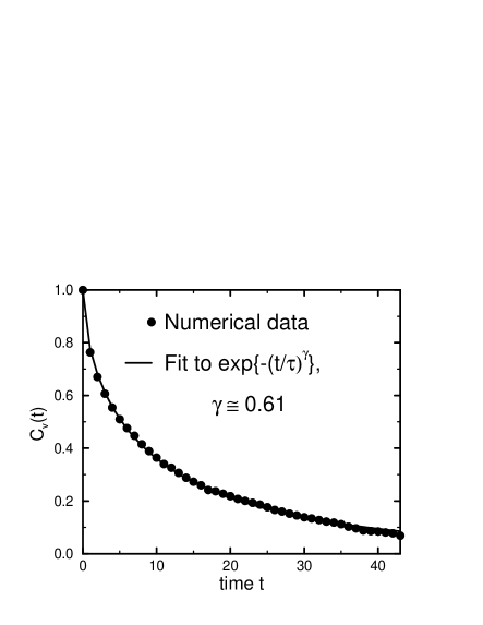
FIG. 7.: Velocity correlations versus time, for the same system in Fig. 6. A stretched exponential is a good fit to the data.

where $\gamma=(d+\zeta_{\parallel})/(z_{\parallel}+d+\zeta_{\parallel})$, suggesting a stretched exponential. The numerical results and the fit to a stretched exponential are shown in Fig. 7. (It should be noted that a comparable fit can also be achieved by a sum of two exponentials.) Assuming that $\zeta_{\parallel}=1$, we arrive at $z\approx 1.3$, which is consistent with the value of $\beta\approx 0.31$ found from the velocity-force relation. Unfortunately, the data becomes noisy at larger values of $t$, due to the finite size of the time window used to extract the correlation function. The small value of $\tau(\approx 10)$ makes it hard to predict the reliability of this estimate, since the power-law prefactors may be large and nonnegligible for such moderate values of $t$. Unfortunately, improving on this simple estimate is difficult as the determination of power-law prefactors requires a number of additional assumptions that are hard to test. Nevertheless, based on the accumulated numerical evidence it can be reasonably argued that $z_{\parallel}$ is between 1 and 4/3, the $O(\epsilon)$ RG prediction.

Computed longitudinal exponents are also in good agreement with results from 1+1 dimensional interface depinning models. Numerical integration of Eq.(IIa) for an elastic interface[29] (no transverse component) has yielded critical exponents $\zeta=0.97\pm 0.05$ and $\nu=1.05\pm 0.1$. Similarly, the force vs. velocity data has been adequately described by both a velocity exponent $\beta=0.24\pm 0.1$ and a logarithmic dependence $v\sim 1/\ln(F-F_{c})$, which corresponds to $\beta=0$. These results provide strong support for our prediction that longitudinal exponents are unchanged when transverse fluctuations are introduced. However, it should also be noted that experiments and various discrete models of interface growth have resulted in scaling behaviors that differ from system to system. A number of different experiments on fluid invasion in porous media[30] give roughness exponents of around 0.8, while imbibition experiments[31, 32] have resulted in $\zeta\approx 0.6$. Some of these results can be explained by the effect of anisotropy, which will be discussed in the next Section. On the other hand, a discrete model studied by Leschhorn[33] gives a roughness exponent of 1.25 at threshold. Since the expansion leading to Eqs.(1) breaks down when $\zeta$ approaches one, it is not clear how to reconcile the results of Leschhhorn’s numerical work[33] with the coarse-grained description of the RG calculation, especially since any model with $\zeta>1$ cannot have a coarse grained description based on gradient expansions.

VIII Discussion and Conclusions

In order to put the results we have found so far in better perspective, it is useful to discuss the effect of nonlinear terms that were ignored earlier, aspects of universality, and possible generalizations to other systems. These issues are discussed below.

A Nonlinear Terms

The leading order nonlinearities in Eq.(II) can be examined by a gradient expansion, being careful to treat terms of $O((\partial_{x}r)^{2},(\partial_{x}r)^{2}\partial_{t}r)$ accurately. After some rearrangement, we arrive at

$$\frac{\eta\partial_{t}{r_{\parallel}}}{\sqrt{1+{s_{\parallel}}^{2}}} = K_{11}\partial_{x}^{2}{r_{\parallel}}+K_{12}\partial_{x}^{2}{r_{\perp}}+{\lambda_{1\parallel}\over 2}{s_{\parallel}}^{2}+{\lambda_{1\perp}\over 2}{s_{\perp}}^{2}$$ (147)

$$\;+\lambda_{1\times}{s_{\parallel}}{s_{\perp}}+F+\tilde{f_{\parallel}}(x,{\bf r},{s_{\parallel}},{s_{\perp}}),$$

$$\frac{\eta\partial_{t}{r_{\perp}}}{\sqrt{1+{s_{\perp}}^{2}}} = K_{21}\partial_{x}^{2}{r_{\parallel}}+K_{22}\partial_{x}^{2}{r_{\perp}}+{\lambda_{2\parallel}\over 2}{s_{\parallel}}^{2}+{\lambda_{2\perp}\over 2}{s_{\perp}}^{2}$$ (149)

$$\;+\lambda_{2\times}{s_{\parallel}}{s_{\perp}}+\tilde{f_{\perp}}(x,{\bf r},{s_{\parallel}},{s_{\perp}}),$$

where ${s_{\parallel}}\equiv\partial_{x}{r_{\parallel}},{s_{\perp}}\equiv\partial_{x}{r_{\perp}}$, and the random forces are

$$\tilde{f_{\parallel}} = \frac{({f_{\parallel}}-{s_{\parallel}}f_{x})}{\sqrt{1+{s_{\parallel}}^{2}}}\cos\phi$$

$$\;+\frac{{s_{\parallel}}{s_{\perp}}{f_{\parallel}}-[1+{s_{\parallel}}^{2}/2-{s_{\perp}}^{2}/2]{f_{\perp}}+{s_{\perp}}f_{x}}{\sqrt{1+{s_{\parallel}}^{2}}}\sin\phi,$$

$$\tilde{f_{\perp}} = \frac{({f_{\perp}}-{s_{\perp}}f_{x})}{\sqrt{1+{s_{\perp}}^{2}}}\cos\phi$$

$$\;+\frac{[1-{s_{\parallel}}^{2}/2+{s_{\perp}}^{2}/2]{f_{\parallel}}-{s_{\parallel}}{s_{\perp}}{f_{\perp}}-{s_{\parallel}}f_{x}}{\sqrt{1+{s_{\perp}}^{2}}}\sin\phi.$$

The remaining parameters are given by

$$F = \Phi_{0}J,$$

$$\lambda_{1\parallel} = -F\sin^{2}\phi,$$

$$\lambda_{1\perp} = -F\cos^{2}\phi,$$

$$\lambda_{1\times} = -F\sin^{2}\phi,$$

$$\lambda_{2\parallel} = F\sin\phi\cos\phi,$$

$$\lambda_{2\perp} = -F\sin\phi\cos\phi,$$

$$\lambda_{2\times} = F\cos^{2}\phi.$$

These equations of motion, and their generalizations to ${\bf x}\in\Re^{d}$, have thus been complicated by two factors: There are orientation-dependent terms, and the mean square of the random forces $\tilde{\Delta}_{\alpha}\equiv\langle\tilde{f_{\alpha}}^{2}\rangle$ also depend on the local orientation of the FL. By naive dimensional counting, it can be immediately seen that $\lambda_{1\parallel}$ and $\lambda_{2\parallel}$ are relevant with respect to the fixed points we have discussed for $d<4$. In the case of Model A (isotropic disorder with $\phi=0$), Eq.(VIII A) further simplifies to

$${\eta\partial_{t}{r_{\parallel}}\over\sqrt{1+{s_{\parallel}}^{2}}} = K\partial_{x}^{2}{r_{\parallel}}-\frac{F}{2}{s_{\perp}}^{2}+F+\frac{{f_{\parallel}}-f_{x}{s_{\parallel}}}{\sqrt{1+{s_{\parallel}}^{2}}},$$ (151)

$${\eta\partial_{t}{r_{\perp}}\over\sqrt{1+{s_{\perp}}^{2}}} = K\partial_{x}^{2}{r_{\perp}}+F{s_{\parallel}}{s_{\perp}}+\frac{{f_{\perp}}-f_{x}{s_{\perp}}}{\sqrt{1+{s_{\perp}}^{2}}}.$$ (152)

Note that the two relevant nonlinearities vanish, and that $\tilde{\Delta}_{\alpha}$ does not depend on orientation up to and including $O(s^{2})$. Dimensional counting suggests that the remaining nonlinear terms are irrelevant and Model A exponents are valid for $d>1$. Many more nonlinear terms become marginal at $d=1$, and the gradient expansion breaks down. It is unlikely for the critical exponents to change their value discontinuously at $d=1$, although logarithmic corrections to scaling exponents are quite possible.

The fixed point investigated here is unstable and only approached at the depinning force. Away from the threshold, critical scaling laws are observed at scales smaller than the correlation length scale $\xi$. Beyond this critical regime, the behavior of Eq. (VIII A) is similar to regular diffusion with white noise (a multicomponent Edwards-Wilkinson (EW) equation[34]), or the generalized KPZ equation[14, 15, 35]). A nonzero $\lambda_{1\parallel}$ of $O(v)$ is generated kinetically in this regime even if the system is initially isotropic with $\phi=0$, due to the terms on the left-hand side of Eq.(VIII Aa). For $d\leq 2$, this nonlinearity is relevant, while for $d>2$, a critical value $\lambda_{c}$ separates a weak-coupling region described by the EW equation from a strong-coupling region described by the (generalized) KPZ equation [14, 15, 35].

When $\phi\neq 0$, even in a fully isotropic medium, the relevant nonlinearities are nonzero, and the system is driven away from the “linear” fixed points. We discuss this and other possibilities next.

B Anisotropy and Universality

We noted earlier that anisotropy plays an important role in determining scaling properties near depinning, even in the absence of nonlinear terms. To fully understand the effects of anisotropy, including nonlinear terms, let us start by considering the simplest prototype of a FL oriented along the $c-$axis of a High $T_{c}$ superconducting single crystal, such as YBCO. For simplicity, assume that the system is completely isotropic in the $y-z$ plane, with $\phi=0$. Then, the motion of the FL is governed by Eqs.(VIII A), and the only important source of anisotropy is due to $\langle{f_{\parallel}}^{2}\rangle=\langle{f_{\perp}}^{2}\rangle\neq\langle f_{x}^{2}\rangle$. This causes the mean square magnitude of $\tilde{f_{\parallel}}$ to depend on the local orientation as,

$\displaystyle\tilde{\Delta}_{\parallel}\approx\langle{f_{\parallel}}^{2}\rangle+\left(\langle f_{x}^{2}\rangle-\langle{f_{\parallel}}^{2}\rangle\right){s_{\parallel}}^{2},$

For interfaces, the depinning force is known to scale with the strength of the disorder[6, 7], i.e. $\tilde{F}_{c}\sim\Delta^{2/(4-d)}$. Thus, $\tilde{\Delta}_{\parallel}$ creates an orientation dependent depinning force[21],

$$F_{c}({s_{\parallel}})\sim{\tilde{\Delta}_{\parallel}}^{2/(4-d)}\sim F_{c}\left(1+\frac{2}{4-d}\frac{\langle f_{x}^{2}\rangle-\langle{f_{\parallel}}^{2}\rangle}{\langle{f_{\parallel}}^{2}\rangle}{s_{\parallel}}^{2}\right).$$ (153)

This leads to a nonzero $\lambda_{1\parallel}$ when the nonlinear corrections in Eq.(VIII A) are taken into account. For interfaces, the depinning transition with a nonzero $\lambda_{1\parallel}$ is thought to be equivalent to directed percolation depinning[21]. Assuming that transverse fluctuations still do not affect longitudinal ones, for $d=1$ the critical exponents $\zeta_{\parallel}$ and $\nu$ are related to the correlation length exponents $\nu_{\parallel}^{(DP)}$ and $\nu_{\perp}^{(DP)}$ of directed percolation through $\nu=\nu_{\parallel}^{(DP)}\approx 1.73$ and $\zeta_{\parallel}=\nu_{\perp}^{(DP)}/\nu_{\parallel}^{(DP)}\approx 0.63$, while the dynamical exponent is $z_{\parallel}=1$. This in turn gives $\beta=(z_{\parallel}-\zeta_{\parallel})\nu=\nu_{\perp}^{(DP)}-\nu_{\parallel}^{(DP)}\approx 0.64$.

Using the connection to interface depinning further, we next consider tilting the FL away from the symmetry axis $c$. In this case, $\langle f_{x}{f_{\parallel}}\rangle$ and $\langle f_{x}{f_{\perp}}\rangle$ are nonzero, and $F_{c}$ depends linearly on $s_{\parallel}$, leading to terms proportional to $\partial_{x}{r_{\parallel}}$ in the equation of motion. These further suppress the roughness exponent to $\zeta_{\parallel}=1/2$[21]. The analysis of transverse fluctuations for these two situations, and many other possible ones, are complicated by the absence of a suitable perturbative treatment. Different types of anisotropy may lead to distinct transverse exponents even while the longitudinal ones remain identical. (Similar to the difference between Models A and B, although the latter is unstable to the inclusion of nonlinear terms.) To systematically search for universality classes, we may start with the most general equation of motion, which has the gradient expansion,

$$\partial_{t}r_{\alpha} = \mu_{\alpha\beta}F_{\beta}+\kappa_{\alpha\beta}\partial_{x}r_{\beta}+K_{\alpha\beta}\partial_{x}^{2}r_{\beta}$$ (155)

$$+\frac{1}{2}\lambda_{\alpha,\beta\gamma}\partial_{x}r_{\beta}\partial_{x}r_{\gamma}+\tilde{f}_{\alpha}(x,{\bf r},\partial_{x}{\bf r},\cdots)+\cdots,$$

and with force-force correlations that depend on $\partial_{x}{\bf r}$. Depending on the presence or absence of various terms allowed by symmetries, these equations encompass many distinct universality classes. The cases that were discussed so far are summarized in Table I.

Situation		$\zeta_{\parallel}$	$\nu$	$z$	$\beta$	$\zeta_{\perp}$	$z_{\perp}$
Anisotropic medium,	$\kappa_{\alpha\beta}\neq 0$	0.5	2	1	1	?	?
generic direction
Anisotropic, FL	$\kappa_{\alpha\beta}=0$	0.63	1.73	1	0.64	?	?
along symmetry axis	$\lambda_{1\parallel}\neq 0$
FL along symmetry	$\kappa_{\alpha\beta}=0$	1	1	1.3	0.3	0	2.3
axis, linear terms	$\phi\neq 0$
only (Model B)
Isotropic medium,	$\kappa_{\alpha\beta}=0$	1	1	1.3	0.3	0.5	2.3
$\phi=0$ (Model A)	$\lambda_{1\parallel}=0$

TABLE I.: Critical exponents corresponding to some of the universality classes associated with vector depinning. Entries in the first two rows are from Ref.[21]: Transverse exponents are not known and these cases may correspond to more than one universality class identified by distinct $\zeta_{\perp},z_{\perp}$.

C Generalizations

In many systems, the dynamics involves a wide range of relaxation times. It is sometimes possible to average over “fast” degrees of freedom to obtain an effective equation of motion for “slow” variables. For example, the motion of atoms in a metal can be described by an effective theory that involves only positions of the ions, assuming that the electronic wavefunction always adjusts to the instantaneus ionic coordinates. Similarly, the critical dynamics of a slowly moving solid-liquid-vapor contact line can be described by assuming that the liquid-vapor interface instantaneusly finds the minimum energy surface dictated by the position of the contact line[36]. The elimination of these additional degrees of freedom may cause effective nonlocal interactions between the remaining modes, which in turn acquire a different dispersion law. For example, in contact line dynamics, the elastic energy associated with a mode of wavevector $q$ is proportional to $|q|$ instead of $q^{2}$. In general, one may consider a situation where the elastic energy is proportional to $|q|^{\sigma}$ for some value of $\sigma$. The scaling analysis can be easily generalized to such cases; the most important change is the modification of the upper critical dimension to $d_{c}=2\sigma$. The exponents can be easily calculated for general $\sigma$, as was done by us for the critical dynamics of a contact line[37] ($\sigma=1$).

The possibility of experimental verification of our results lies in the ability to accurately measure the motion of individual FLs and the noise spectra (for both normal and Hall voltages) generated by FL motion. Very recently, there have been successful experiments that detected the thermal motion of individual FLs at nominally zero magnetic field and bulk current using SQUID probes, and analyzed the noise correlation between the two ends of the FL[38]. A refinement of such techniques may eventually enable a direct comparison of theoretical results with experiments. For example, it is known that the Hall angle changes sign as a function of temperature in certain superconductors[39]. It would be particularly interesting to observe the increase in transverse roughness (thus the Hall Voltage noise) as the Hall angle approaches zero. Ultimately, it is very desirable to understand the properties of many FLs (solid or glass) near depinning, especially since this situation has much more experimental and technological relevance. One should then start from a coarse-grained theory for the displacements ${\bf u}({\bf x},t)$ of the FLs with respect to their equilibrium positions in the Abrikosov lattice and hope to establish a similar RG scheme. However, there are certainly additional complications, such as entanglement[40] and plasticity[41] effects, which are difficult to incorporate in such an approach.

A The Gaussian Theory

In this appendix, we compute all nonzero expectation values for the Gaussian theory, described by the effective action $\tilde{S}_{0}$ in Eq.(100). This is accomplished by inverting the quadratic form, as

$$\left[\matrix{\langle{\bf\hat{R}}({\bf q},\omega){\bf\hat{R}}^{T}(-{\bf q},-\omega)\rangle_{c}&\langle{\bf\hat{R}}({\bf q},\omega){\bf R}^{T}(-{\bf q},-\omega)\rangle_{c}\cr\cr\langle{\bf R}({\bf q},\omega){\bf\hat{R}}^{T}(-{\bf q},-\omega)\rangle_{c}&\langle{\bf R}({\bf q},\omega){\bf R}^{T}(-{\bf q},-\omega)\rangle_{c}\cr}\right] = \left[\matrix{-{\bf C}(\omega)&{\bf G}^{-1}({\bf q},\omega)\cr\cr{{\bf G}^{{\dagger}}}^{-1}({\bf q},\omega)&{\bf 0}\cr}\right]^{-1}$$

$$=\left[\matrix{{\bf 0}&{\bf G}^{{\dagger}}({\bf q},\omega)\cr\cr{\bf G}({\bf q},\omega)&{\bf G}({\bf q},\omega){\bf C}(\omega){\bf G}^{{\dagger}}({\bf q},\omega)\cr}\right].$$

For the case of Model A, the individual matrices are diagonal and the correlation functions can be calculated easily, as given in Eqs.(VI A). For the more general case of Model B, let us first consider the $v\to 0$ limit. Since $R_{\perp}$ occurs in the combination $R_{\perp}/v$, expectation values $\langle{\hat{R}}_{\alpha}R_{\perp}\rangle$ and $\langle R_{\alpha}R_{\perp}\rangle$ contribute at most $O(v)$ at the  momentum-shell integration step. Thus, the contractions that are important for the momentum-shell integration are $\langle{\hat{R}}_{\parallel}R_{\parallel}\rangle$ and $\langle R_{\parallel}R_{\parallel}\rangle$. Setting $v=0$ and inverting the matrix yields

$${\bf G}({\bf q},\omega) = \left[\matrix{K_{11}q^{2}-i\omega A_{11}&+i\omega A_{12}\cr K_{21}q^{2}-i\omega A_{21}&-i\omega A_{22}\cr}\right]^{-1}=\frac{1}{{K_{\parallel}}q^{2}-i\omega\rho_{\parallel}}\left[\matrix{1&\kappa\cr\cdots&\cdots\cr}\right],$$ (A1)

$${\bf G}{\bf C}{\bf G}^{{\dagger}}({\bf q},\omega) = \frac{1}{{K_{\parallel}}^{2}q^{4}+\omega^{2}\rho_{\parallel}^{2}}\left[\matrix{\tilde{C}(\omega)&\cdots\cr\cdots&\cdots\cr}\right],$$ (A2)

which leads to Eqs.(VI B). To determine the full form of the correlation functions in a renormalized Gaussian theory, we need to perform a full matrix inversion. In the small $v$ limit we obtain

$$\langle|R_{\parallel}({\bf q},\omega)|^{2}\rangle = \frac{1}{|\det G^{-1}|^{2}}\left\{A_{22}^{2}\omega^{2}{\tilde{C}}(\omega)-vq^{2}\omega(K_{12}A_{22}+K_{22}A_{12}){\rm Im}[C_{\times}(\omega)]\right.$$

$$\qquad\qquad\left.+v^{2}q^{4}\left[K_{22}^{2}C_{\parallel}(\omega)-K_{22}K_{12}{\rm Re}C_{\times}(\omega)+K_{12}^{2}C_{\perp}(\omega)\right]\right\},$$

where

$$|\det G^{-1}|^{2} \approx [{K_{\parallel}}^{2}q^{4}+\rho_{\parallel}^{2}\omega^{2}]\left[v^{2}q^{4}\left([K_{11}K_{22}-K_{21}K_{12}]/{K_{\parallel}}\right)^{2}+A_{22}^{2}\omega^{2}\right].$$

Similarly,

$$\langle|R_{\perp}({\bf q},\omega)|^{2}\rangle = \frac{v^{2}}{|\det G^{-1}|^{2}}\left\{\left(K_{21}^{2}C_{\parallel}(\omega)-K_{21}K_{11}{\rm Re}[C_{\times}(\omega)]+K_{11}^{2}C_{\perp}(\omega)\right)q^{4}\right.$$

$$\qquad\qquad\qquad\qquad-\omega q^{2}(K_{11}A_{21}-K_{21}A_{11}){\rm Im}[C_{\times}(\omega)]$$

$$\qquad\qquad\qquad\qquad\left.+\omega^{2}\left(A_{21}^{2}C_{\parallel}(\omega)-A_{21}A_{11}{\rm Re}[C_{\times}(\omega)]+A_{11}^{2}C_{\perp}(\omega)\right)\right\}.$$

At the fixed point found for Model B, Eqs.(144) are satisfied, and the correlation functions simplify to

$$\langle|R_{\parallel}({\bf q},\omega)|^{2}\rangle = \frac{{\tilde{C}}(\omega)}{{K_{\parallel}}^{2}q^{4}+\rho_{\parallel}^{2}\omega^{2}}{\cal F}_{\parallel}\left({K_{\perp}q^{2}\over(\omega/v)\rho_{\perp}}\right),$$ (A3)

$$\langle|R_{\perp}({\bf q},\omega)|^{2}\rangle = \frac{{\tilde{C}}(\omega)}{4\left[{K_{\perp}}^{2}q^{4}+\rho_{\perp}^{2}(\omega/v)^{2}\right]}{\cal F}_{\perp}\left({K_{\parallel}q^{2}\over\omega\rho_{\parallel}}\right),$$ (A4)

where

$$K_{\perp}= \left|\displaystyle\frac{K_{11}K_{22}-K_{21}K_{12}}{K_{11}-\kappa K_{21}}\right|,\qquad\qquad\qquad\qquad\rho_{\perp} =\left|\frac{K_{11}+\kappa K_{21}}{K_{11}-\kappa K_{21}}\right|A_{22},$$

$${\cal F}_{\parallel}(x)= \left[{1+x^{2}\left(\displaystyle\frac{(K_{22}-K_{12}/\kappa)K_{\parallel}}{2(K_{11}K_{22}-K_{21}K_{12})}\right)^{2}}\right]\bigg{/}\left[{1+x^{2}}\right] =\cases{1,&$x\ll 1$\cr{\rm const},&$x\gg 1$.}$$

$${\cal F}_{\perp}(x)= \left[{1+\displaystyle{1\over x^{2}}\left(\displaystyle\frac{K_{11}+\kappa K_{21}}{K_{11}-\kappa K_{21}}\frac{A_{11}-\kappa A_{21}}{A_{11}+\kappa A_{21}}\right)^{2}}\right]\bigg{/}\left[{1+\displaystyle{1\over x^{2}}}\right] =\cases{{\rm const},&$x\ll 1$,\cr 1,&$x\gg 1$.}$$

The functions ${\cal F}_{\alpha}$ describe crossovers of the overall amplitudes of the correlations, due to the coupling between longitudinal and transverse modes.

B Vertex Renormalization

In this appendix, we derive recursion relations for the renormalized vertex functions $U_{\alpha,n}(u)\equiv C_{\alpha}^{(n)}(u)$. Let us start by considering $U_{\alpha,n}(u)$ for a given $n$. As usual, we split the fields ${\bf R}={\bf R}^{<}+{\bf R}^{>}$ and ${\bf\hat{R}}={\bf\hat{R}}^{<}+{\bf\hat{R}}^{>}$, where fields with the superscript “$>$” correspond to fluctuations within the momentum shell $\Lambda e^{-\delta\ell}<q<\Lambda$, which are averaged over. In evaluating $\langle e^{\cal U}\rangle_{0}^{>}$, we encounter two types of nonzero contractions,

$$\left<{\hat{R}}_{\parallel}^{>}({\bf q},t)R_{\parallel}^{>}(-{\bf q},t^{\prime})\right> = \frac{1}{A_{11}}\exp\left[-\frac{Kq^{2}(t^{\prime}-t)}{A_{11}}\right]\Theta(t^{\prime}-t)$$

$$\approx \frac{1}{K\Lambda^{2}}\delta(t-t^{\prime}),$$

$$\left<R_{\parallel}^{>}({\bf q},t)R_{\parallel}^{>}(-{\bf q},t^{\prime})\right> \approx \frac{1}{K^{2}\Lambda^{4}}U_{\alpha,0}\left(v(t-t^{\prime})\right),$$

within the momentum shell $\Lambda e^{-\delta\ell}<q<\Lambda$, and for time scales $t-t^{\prime}\sim O(1/v)$. (From now on, we suppress the subscript 0 for notational simplicity.) Contributions to the renormalization of $U_{\alpha,n}$ come from both $\langle{\cal U}\rangle^{>}$ and $\langle{\cal U}^{2}\rangle_{c}^{>}$, as

$$\langle{\cal U}\rangle^{>} = \sum_{\alpha}\frac{1}{2!(n+2)!}\int d^{d}x\,dt_{1}dt_{2}\,U_{\alpha,n+2}(1-2)\left<{\hat{R}}_{\alpha}(1){\hat{R}}_{\alpha}(2)[R_{\parallel}(1)-R_{\parallel}(2)]^{n+2}\right>^{>}+\cdots$$

$$= \sum_{\alpha}\frac{1}{2!(n+2)!}{n+2\choose 2}\int d^{d}x\,dt_{1}dt_{2}\,U_{\alpha,n+2}(1-2){\hat{R}}^{<}_{\alpha}(1){\hat{R}}^{<}_{\alpha}(2)$$

$$\qquad\qquad\qquad\qquad\qquad\qquad\times[R^{<}_{\parallel}(1)-R^{<}_{\parallel}(2)]^{n}\left<[R^{>}_{\parallel}(1)-R^{>}_{\parallel}(2)]^{2}\right>+\cdots,$$

with obvious abbreviations for the arguments of $U,R,{\hat{R}}$. Evaluating the expectation values, we get

$$\left<[R^{>}_{\parallel}(1)-R^{>}_{\parallel}(2)]^{2}\right> = \int\limits^{>}{{d^{d}q\over(2\pi)^{d}}\,}\left\{\left<R_{\parallel}^{>}({\bf q},t_{1})R_{\parallel}^{>}(-{\bf q},t_{1})\right>+\left<R_{\parallel}^{>}({\bf q},t_{2})R_{\parallel}^{>}(-{\bf q},t_{2})\right>\right.$$ (B2)

$$\qquad\qquad\qquad\qquad\left.-2\left<R_{\parallel}^{>}({\bf q},t_{1})R_{\parallel}^{>}(-{\bf q},t_{2})\right>\right\}$$

$$= 2\delta\ell\frac{\Lambda^{d}S_{d}}{(2\pi)^{d}K^{2}\Lambda^{4}}[U_{\parallel,0}(0)-U_{\parallel,0}(v(t_{1}-t_{2}))],$$ (B3)

where $\int^{>}$ denotes integration over the momentum shell and $S_{d}$ is the surface area of a unit sphere in $d$-dimensions. Thus, the correction to $U^{<}_{\alpha,n}(u)$ from $\langle{\cal U}\rangle^{>}$ is equal to

$\displaystyle\delta\ell K_{d}U_{\alpha,n+2}(u)[U_{\parallel,0}(0)-U_{\parallel,0}(u)],$

where $K_{d}\equiv\Lambda^{d-4}S_{d}/[(2\pi)^{d}K^{2}]$. The contributions from $\langle{\cal U}^{2}\rangle_{c}^{>}$ are similarly calculated, as

$$\langle{\cal U}^{2}\rangle_{c}^{>}\!\! = \sum_{\alpha,\gamma}\sum_{m=1}^{n+1}\frac{1}{2!m!2!(n+2-m)!}\int d^{d}x\,dt_{1}dt_{2}\int d^{d}x^{\prime}\,dt_{1}^{\prime}dt_{2}^{\prime}\,U_{\alpha,m}(1-2)U_{\gamma,n+2-m}(1^{\prime}-2^{\prime})$$ (B5)

$$\qquad\qquad\times\left<{\hat{R}}_{\alpha}(1){\hat{R}}_{\alpha}(2){\hat{R}}_{\gamma}(1^{\prime}){\hat{R}}_{\gamma}(2^{\prime})[R_{\parallel}(1)-R_{\parallel}(2)]^{m}[R_{\parallel}(1^{\prime})-R_{\parallel}(2^{\prime})]^{n+2-m}\right>^{>}+\cdots$$

$$= \sum_{m=1}^{n+1}\frac{1}{2!(m-1)!2!(n+1-m)!}\int d^{d}x\,dt_{1}dt_{2}\int d^{d}x^{\prime}\,dt_{1}^{\prime}dt_{2}^{\prime}\,U_{\parallel,m}(1-2)U_{\parallel,n+2-m}(1^{\prime}-2^{\prime})$$ (B11)

$$\qquad\qquad\times[R^{<}_{\parallel}(1)-R^{<}_{\parallel}(2)]^{m-1}[R^{<}_{\parallel}(1^{\prime})-R^{<}_{\parallel}(2^{\prime})]^{n+1-m}$$

$$\qquad\qquad\times\left<{\hat{R}}_{\parallel}(1){\hat{R}}_{\parallel}(2){\hat{R}}_{\parallel}(1^{\prime}){\hat{R}}_{\parallel}(2^{\prime})[R^{>}_{\parallel}(1)-R^{>}_{\parallel}(2)][R^{>}_{\parallel}(1^{\prime})-R^{>}_{\parallel}(2^{\prime})]\right>^{>}$$

$$+2\sum_{\alpha}\sum_{m=1}^{n}\frac{1}{2!m!2!(n+2-m)!}{n+2-m\choose 2}\int d^{d}x\,dt_{1}dt_{2}\int d^{d}x^{\prime}\,dt_{1}^{\prime}dt_{2}^{\prime}$$

$$\qquad\qquad\times U_{\alpha,m}(1-2)U_{\parallel,n+2-m}(1^{\prime}-2^{\prime}){\hat{R}}^{<}_{\alpha}(1^{\prime}){\hat{R}}^{<}_{\alpha}(2^{\prime})[R^{<}_{\parallel}(1)-R^{<}_{\parallel}(2)]^{m}$$

$$\qquad\qquad\times[R^{<}_{\parallel}(1^{\prime})-R^{<}_{\parallel}(2^{\prime})]^{n-m}\left<{\hat{R}}^{>}_{\parallel}(1){\hat{R}}^{>}_{\parallel}(2)[R^{>}_{\parallel}(1^{\prime})-R^{>}_{\parallel}(2^{\prime})]^{2}\right>+\cdots.$$

The evaluations of the expectation values are tedious but straightforward. As an example, let us evaluate the second half of Eq.(B5) explicitly. First of all,

$$\left<{\hat{R}}^{>}_{\parallel}(1){\hat{R}}^{>}_{\parallel}(2)[R^{>}_{\parallel}(1^{\prime})-R^{>}_{\parallel}(2^{\prime})]^{2}\right>=$$

$$= \left<{\hat{R}}^{>}_{\parallel}(1)R^{>}_{\parallel}(1^{\prime})\right>\left<{\hat{R}}^{>}_{\parallel}(2)R^{>}_{\parallel}(1^{\prime})\right>+\left<{\hat{R}}^{>}_{\parallel}(1)R^{>}_{\parallel}(2^{\prime})\right>\left<{\hat{R}}^{>}_{\parallel}(2)R^{>}_{\parallel}(2^{\prime})\right>$$

$$\quad-2\left<{\hat{R}}^{>}_{\parallel}(1)R^{>}_{\parallel}(1^{\prime})\right>\left<{\hat{R}}^{>}_{\parallel}(2)R^{>}_{\parallel}(2^{\prime})\right>-2\left<{\hat{R}}^{>}_{\parallel}(1)R^{>}_{\parallel}(2^{\prime})\right>\left<{\hat{R}}^{>}_{\parallel}(2)R^{>}_{\parallel}(2^{\prime})\right>.$$

The first two terms do not contribute to $U^{<}_{\alpha,n}(u)$, since they are proportional to $\delta(t_{1}-t_{1}^{\prime})\delta(t_{2}-t_{1}^{\prime})$ and $\delta(t_{1}-t_{2}^{\prime})\delta(t_{2}-t_{2}^{\prime})$ respectively. (These delta functions force $t_{1}$ to be equal to $t_{2}$. Since the expectation value is multiplied by $[R^{<}_{\parallel}(1)-R^{<}_{\parallel}(2)]^{m}$, the final contribution is zero.) The last two terms are equal to

$\displaystyle-2\int\limits^{>}{{d^{d}q\over(2\pi)^{d}}\,}\int\limits^{>}\frac{d^{d}q^{\prime}}{(2\pi)^{d}}[\delta(t_{1}-t_{1}^{\prime})\delta(t_{2}-t_{2}^{\prime})+\delta(t_{1}-t_{2}^{\prime})\delta(t_{2}-t_{1}^{\prime})]\frac{\exp\{i({\bf q}+{\bf q}^{\prime})\cdot({\bf x}-{\bf x}^{\prime})\}}{(Kq^{2})(Kq^{{}^{\prime}2})}.$

Integrating over $t_{1}^{\prime}$, $t_{2}^{\prime}$, ${\bf x}^{\prime}$ (which yields $\delta^{d}({\bf q}+{\bf q}^{\prime})$) and subsequently over ${\bf q}^{\prime}$, the second half of Eq.(B5) becomes

$$-\sum_{\alpha}\sum_{m=1}^{n}\frac{1}{2!n!}{n\choose m} \int d^{d}xdt_{1}dt_{2}{\hat{R}}^{<}_{\alpha}(1){\hat{R}}^{<}_{\alpha}(2)[R^{<}_{\parallel}(1)-R^{<}_{\parallel}(2)]^{n}\int\limits^{>}{{d^{d}q\over(2\pi)^{d}}\,}\frac{1}{K^{2}q^{4}}$$

$$\times\left\{U_{\alpha,m}(1-2)U_{\parallel,n+2-m}(1-2)+(-1)^{n-m}U_{\alpha,m}(1-2)U_{\parallel,n+2-m}(2-1)\right\}.$$

The first half of Eq.(B5) can be evaluated similarly. The full contribution to $U^{<}_{\alpha,n}(u)$ from $\langle{\cal U}^{2}\rangle_{c}^{>}$ is thus equal to

$$-\delta\ell K_{d}\left\{\delta_{\alpha,\parallel}\sum_{m=1}^{n+1}{n\choose m-1}\right. (-1)^{n+2-m}U_{\parallel,m}(u)U_{\parallel,n+2-m}(-u)$$

$$+\sum_{m=1}^{n}{n\choose m} \left.{1\over 2}\left[U_{\alpha,m}(u)U_{\parallel,n+2-m}(u)+(-1)^{n+2-m}U_{\alpha,m}(u)U_{\parallel,n+2-m}(-u)\right]\right\}.$$

(In the expansion of $\langle e^{\cal U}\rangle_{c}^{>}$, there is a factor of $1/2$ in front of $\langle{\cal U}^{2}\rangle_{c}^{>}$.) Adding all contributions, the effective vertex function $U^{<}_{\parallel,n}(u)$ is found to be

$$U^{<}_{\parallel,n}(u)=U_{\parallel,n}(u)+\delta\ell K_{d}\left\{U_{\parallel,n+2}(u)U_{\parallel,0}(0)-\sum_{m=0}^{n+1}{n+1\choose m}U_{\parallel,m}(u)U_{\parallel,n+2-m}(u)\right\},$$ (B12)

provided that

$$U_{\alpha,m}(u)=(-1)^{m}U_{\alpha,m}(-u).$$ (B13)

Under the scale transformation (105), which brings the momentum cutoff to its original value, we see that $u\to(1+\zeta_{\parallel}\delta\ell)u$. Thus, the renormalized vertex function is given by

$$\tilde{U}_{\parallel,n}(u)\equiv U_{\parallel,n}(u)+\delta\ell\frac{\partial U_{\parallel,n}(u)}{\partial\ell}=U^{<}_{\parallel,n}\left((1+\zeta_{\parallel}\delta\ell)u\right)\{1+\delta\ell[d+2z_{\parallel}+2(\theta_{\parallel}-d)+n\zeta_{\parallel}]\}.$$ (B14)

Keeping only terms linear in $\delta\ell$, and identifying $U_{\parallel,n}(u)$ with the $n$th derivative of $C_{\parallel}(u)$, we finally obtain the differential recursion relation for $C_{\parallel}(u)$:

$$\frac{\partial C_{\parallel}(u)}{\partial\ell}=[\epsilon+2\theta_{\parallel}+2(z_{\parallel}-2)]C_{\parallel}(u)+\zeta_{\parallel}uC^{\prime}_{\parallel}(u)-K_{d}\left\{[C^{\prime}_{\parallel}(u)]^{2}+[C_{\parallel}(u)-C_{\parallel}(0)]C^{\prime\prime}_{\parallel}(u)\right\}.$$ (B15)

Note that the identification of $U_{\parallel,n}(u)$ with the $n$th derivative of $C_{\parallel}(u)$ is self-consistent, since recursion relations for $U_{\parallel,n}(u)$ are correctly recovered by taking $n$ derivatives of Eq.(B15). Also, Eq.(B13) is automatically satisfied when this identification is made since $C_{\parallel}(u)=C_{\parallel}(-u)$.

A similar computation can be performed for $C_{\perp}(u)$, yielding

$$U^{<}_{\perp,n}(u)=U_{\perp,n}(u)+\delta\ell K_{d}\left\{U_{\perp,n+2}(u)U_{\parallel,0}(0)-\sum_{m=0}^{n}{n\choose m}U_{\perp,n+2-m}(u)U_{\parallel,m}(u)\right\}.$$ (B16)

Upon rescaling, the renormalized vertex function is

$$\tilde{U}_{\perp,n}(u)\equiv U_{\perp,n}(u)+\delta\ell\frac{\partial U_{\perp,0}(u)}{\partial\ell}=U^{<}_{\perp,n}\left((1+\zeta_{\parallel}\delta\ell)u\right)\{1+\delta\ell[d+2z_{\parallel}+2(\theta_{\perp}-d)+n\zeta_{\parallel}]\}.$$ (B17)

Thus, we obtain the recursion relation

$$\frac{\partial C_{\perp}(u)}{\partial\ell}=[\epsilon+2\theta_{\perp}+2(z_{\parallel}-2)]C_{\perp}(u)+\zeta_{\parallel}uC^{\prime}_{\perp}(u)-K_{d}\left\{[C_{\parallel}(u)-C_{\parallel}(0)]C^{\prime\prime}_{\perp}(u)\right\}.$$ (B18)

C Higher-Order Diagrams

In this appendix, we show that the sum of all contributions to the renormalization of $C_{\perp}(u)$ from the momentum shell integration step vanish in the limit $u\to 0^{+}$. This was already explicitly demonstrated for the leading order contributions that come from $\langle{\cal U}\rangle_{c}$ and $\langle{\cal U}^{2}\rangle_{c}$. Since the only nonzero contractions involve $R_{\parallel}$ and ${\hat{R}}_{\parallel}$, all contributions to the renormalization of $C_{\perp}(v(t-t^{\prime}))$ due to $\left<{\cal U}^{m}\right>_{c}$ arise from terms of the form

$$\left<{\cal U}^{m}\right>_{c} = \sum_{n=2}^{\infty}\int{d^{d}\!x\,}{dt\,}dt^{\prime}\frac{U_{\perp,n}(v(t-t^{\prime}))}{2!n!}{\hat{R}}^{<}_{\perp}(t){\hat{R}}^{<}_{\perp}(t^{\prime})\int\left[\prod_{i=1}^{m-1}d^{d}\!x_{i}\,dt_{i}\,dt_{i}^{\prime}\,\frac{U_{\parallel,n_{i}}(v(t_{i}-t_{i}^{\prime}))}{2!n_{i}!}\right]$$

$$\qquad\times\left<[R_{\parallel}^{>}({\bf x},t)-R_{\parallel}^{>}({\bf x},t^{\prime})]^{n}\prod_{i=1}^{m-1}{\hat{R}}_{\parallel}^{>}({\bf x}_{i},t_{i}){\hat{R}}_{\parallel}^{>}({\bf x}_{i},t^{\prime}_{i})[R_{\parallel}^{>}({\bf x}_{i},t_{i})-R_{\parallel}^{>}({\bf x}_{i},t^{\prime}_{i})]^{n_{i}}\right>_{c}+\cdots.$$

The expectation value clearly goes to zero as $(t-t^{\prime})^{n}$ in the $t\to t^{\prime+}$ limit. This gives us the desired result that $C_{\perp}(0)$ is unrenormalized to all orders in perturbation theory.

D High-frequency structure of $U_{\parallel,2}$

In this appendix, we shall demonstrate that there are no $v^{-1}$ divergences in the renormalization of $A_{11}$, at least to $O(\epsilon)$. In order to do this, we examine the full form of the bare vertex function $U_{\parallel,2}$ obtained from MF theory,

$\displaystyle U_{\parallel,2}(t_{1},t_{2};t^{\prime}_{1},t^{\prime}_{2})=\frac{\partial^{2}\left<\overline{r}_{\parallel}(t_{1})\overline{r}_{\parallel}(t_{2})\right>_{MF,c}}{\partial\varepsilon_{\parallel}(t^{\prime}_{1})\partial\varepsilon_{\parallel}(t^{\prime}_{2})}.$

The low-frequency analysis of this vertex function gives a result proportional to $1/v$ when all times are within $O(1)$ of each other. This may potentially give an $O(1/v)$ contribution to the renormalization of $A_{11}$. Indeed, an external impulse of magnitude $\varepsilon$ right before a “jump” (the fast motion between consequent local minima) shifts the jump time by $\varepsilon/\eta$ and creates a response of $O(1/v)$ right after the jump takes place. However, an impulse right after a jump does not affect the jump time and creates a response of only $O(1)$. Thus a singular response is seen if all times are in the vicinity of a jump, say, at time $t_{J}$. $U_{\parallel,2}(t_{1},t_{2};t^{\prime}_{1},t^{\prime}_{2})$ can be as large as $O(v^{-2})$ if $t^{\prime}_{1}$ and $t^{\prime}_{2}$ are both slightly less than $t_{J}$, and $t_{1}$ and $t_{2}$ are both slightly greater than $t_{J}$. Considering that the probability of being close to a jump is $v$, this term can potentially contribute as much as $O(v^{-1})$ to the renormalization of $A_{11}$ upon statistical time-averaging. A careful analysis, and explicit evaluation of this vertex in the case of a periodic potential[42], show that this is the only way a singularity may occur in the RG contributions. However, when the times $t^{\prime}_{1},t^{\prime}_{2}$ of fields $R_{\parallel}$ are smaller than the times $t_{1},t_{2}$ of fields ${\hat{R}}_{\parallel}$, the contraction $\left<{\hat{R}}_{\parallel}(t_{i})R_{\parallel}(t^{\prime}_{j})\right>_{0}$ which appears in the RG contribution is identically zero due to the causality of the propagator. Therefore, the singular part of $C_{\parallel}^{*^{\prime\prime}}(0)$ does not enter the renormalization of $A_{11}$ (or $\rho_{\parallel}$ in the case of Model B) to one-loop order.

E Renormalization of Model B

Details of the RG calculation for Model B are presented in this appendix. For the sake of brevity, we shall only consider the renormalization of the parameters in the Gaussian theory, i.e. the propagator, and the two-point correlation functions $U_{\parallel,0}(u)$, $U_{\perp,0}(u)$, $U_{\times,0}(u)$. The renormalization of higher-order vertex functions are again related to derivatives of $C_{\alpha}$ through $U_{\alpha,n}(u)\equiv C_{\alpha}^{(n)}(u)$.

Nonzero contractions involved in the calculation are given in Eqs.(VI B). The parameters $A_{12},A_{22}$ (thus $\kappa$), and $K_{\alpha\gamma}$ (thus $K_{\parallel},K_{\perp}$, and $\rho_{\perp}$) do not get contributions from the momentum shell integration, and give rise to exponent identities discussed in the text. On the other hand, $A_{11}$ and $A_{21}$ (thus $\rho_{\parallel}$), as well as the functions $C_{\alpha}(u)$, are renormalized. Let us start by looking at the renormalization of two-point correlation functions $C_{\alpha}(u)$. By definition, $C_{\parallel}(u)=C_{\parallel}(-u)$ and $C_{\perp}(u)=C_{\perp}(-u)$, but $C_{\times}(u)\neq C_{\times}(-u)$ in general. It is convenient to write $C_{\times}(u)$ in terms of its even and odd parts $C_{\times S}(u)$ and $C_{\times A}(u)$ respectively, and follow their renormalization separately.

The momentum shell integration procedure is similar to the one presented in Appendix B, albeit more cumbersome due to many more nonzero contractions. Nevertheless, carrying out the computation yields

$$C^{<}_{\alpha}(u)=C_{\alpha}(u)-\delta\ell K_{d}{\cal I}_{\alpha}(u),$$ (E1)

for $u>0$, where

$${\cal I}_{\parallel}(u) = C_{\parallel}^{\prime\prime}(u)[{\tilde{C}}(u)-{\tilde{C}}(0^{+})]+C_{\parallel}^{\prime}(u){\tilde{C}}^{\prime}(u)$$ (E4)

$$\quad-\kappa^{2}\left\{C_{\parallel}^{\prime}(u)C_{\perp}^{\prime}(u)-[C_{\times S}^{\prime}(u)/2]^{2}+[C_{\times A}^{\prime}(u)/2]^{2}\right\}$$

$$\quad+\kappa C_{\times A}(u)\left\{C_{\parallel}^{\prime}(0^{+})+\kappa[C_{\times A}^{\prime}(0^{+})/2]\right\},$$

$${\cal I}_{\perp}(u) = C_{\perp}^{\prime\prime}(u)[{\tilde{C}}(u)-{\tilde{C}}(0^{+})]+C_{\perp}^{\prime}(u){\tilde{C}}^{\prime}(u)$$ (E7)

$$\quad-\left\{C_{\parallel}^{\prime}(u)C_{\perp}^{\prime}(u)-[C_{\times S}^{\prime}(u)/2]^{2}+[C_{\times A}^{\prime}(u)/2]^{2}\right\}$$

$$\quad+C_{\times A}(u)\left\{[C_{\times A}^{\prime}(0^{+})/2]-\kappa C_{\perp}^{\prime}(0^{+})\right\},$$

$${\cal I}_{\times S}(u) = C_{\times S}^{\prime\prime}(u)[{\tilde{C}}(u)-{\tilde{C}}(0^{+})]+C_{\times S}^{\prime}(u){\tilde{C}}^{\prime}(u)$$ (E10)

$$\quad+2\kappa\left\{C_{\parallel}^{\prime}(u)C_{\perp}^{\prime}(u)-[C_{\times S}^{\prime}(u)/2]^{2}+[C_{\times A}^{\prime}(u)/2]^{2}\right\}$$

$$\quad-C_{\times A}(u)\left\{C_{\parallel}^{\prime}(0^{+})+\kappa C_{\times A}^{\prime}(0^{+})-\kappa^{2}C_{\perp}^{\prime}(0^{+})\right\},$$

$${\cal I}_{\times A}(u) = C_{\times A}^{\prime\prime}(u)[{\tilde{C}}(u)-{\tilde{C}}(0^{+})]+C_{\times A}^{\prime}(u){\tilde{C}}^{\prime}(u)$$ (E13)

$$\quad+4\kappa\left\{C_{\parallel}^{\prime}(u)C_{\perp}^{\prime}(0^{+})-C_{\parallel}^{\prime}(0^{+})C_{\perp}^{\prime}(u)\right\}$$

$$\quad-C_{\times S}^{\prime}(u)\left\{C_{\parallel}^{\prime}(0^{+})+\kappa C_{\times A}^{\prime}(u)-\kappa^{2}C_{\perp}^{\prime}(0^{+})\right\}.$$

Thus, the renormalization of ${\tilde{C}}(u)$ is given by

$${\tilde{C}}^{<}(u)={\tilde{C}}(u)-\delta\ell K_{d}\left\{{\tilde{C}}^{\prime\prime}(u)[{\tilde{C}}(u)-{\tilde{C}}(0^{+})]+[{\tilde{C}}^{\prime}(u)]^{2}\right\},$$ (E14)

which leads to the functional recursion relation

$$\frac{\partial{\tilde{C}}(u)}{\partial\ell}=[\epsilon+2\theta_{\parallel}+2(z_{\parallel}-2)]{\tilde{C}}(u)+\zeta_{\parallel}u{\tilde{C}}^{\prime}(u)-K_{d}\left\{[{\tilde{C}}^{\prime}(u)]^{2}+[{\tilde{C}}(u)-{\tilde{C}}(0)]{\tilde{C}}^{\prime\prime}(u)\right\}.$$ (E15)

This is identical to Eq.(B15), with the substitution $C_{\parallel}(u)\to{\tilde{C}}(u)$. It is straightforward to verify that there exists a fixed point where individual matrix elements $C_{\alpha}(u)$ satisfy Eq.(144). ($C_{\times A}(u)=0$ at this fixed point.)

Let us next examine the renormalization of $\rho_{\parallel}$. Leading order contributions come from $\langle{\cal U}\rangle^{>}_{0}$, and a calculation along the lines presented in Sec.VI gives

$$A_{11}^{<} = A_{11}-\delta\ell\frac{S_{d}\Lambda^{d}}{(2\pi)^{d}\rho_{\parallel}}\int\limits_{0}^{\infty}d\tilde{t}\,\tilde{t}\,e^{-K_{\parallel}\Lambda^{2}\tilde{t}/\rho_{\parallel}}\left[C^{\prime\prime}_{\parallel}(v\tilde{t}\,)+{\kappa\over 2}C^{\prime\prime}_{\times}(v\tilde{t}\,)\right],$$

$$A_{21}^{<} = A_{21}-\delta\ell\frac{S_{d}\Lambda^{d}}{(2\pi)^{d}\rho_{\parallel}}\int\limits_{0}^{\infty}d\tilde{t}\,\tilde{t}\,e^{-K_{\parallel}\Lambda^{2}\tilde{t}/\rho_{\parallel}}\left[{1\over 2}C^{\prime\prime}_{\times}(-v\tilde{t}\,)+\kappa C^{\prime\prime}_{\perp}(v\tilde{t}\,)\right],$$

which can be combined to yield

$$\rho_{\parallel}^{<}=\rho_{\parallel}-\delta\ell\frac{S_{d}\Lambda^{d}}{(2\pi)^{d}\rho_{\parallel}}\int\limits_{0}^{\infty}d\tilde{t}\,\tilde{t}\,e^{-K_{\parallel}\Lambda^{2}\tilde{t}/\rho_{\parallel}}{\tilde{C}}^{\prime\prime}(v\tilde{t}\,).$$ (E16)

The fixed-point function ${\tilde{C}}^{*}(u)$ is identical to that of $C^{*}_{\parallel}(u)$ in Model A, and its behavior near $u=0$ is also given by Eq.(129). Thus, we obtain

$\displaystyle\rho_{\parallel}^{<}=\rho_{\parallel}-\delta\ell\rho_{\parallel}K_{d}{\tilde{C}}^{\prime\prime}(0^{+})=\rho_{\parallel}[1-\delta\ell(2\epsilon/9)]$

which leads to the recursion relation

$$\frac{\partial\rho_{\parallel}}{\partial\ell}=\rho_{\parallel}[\theta_{\parallel}+\zeta_{\parallel}-2\epsilon/9].$$ (E17)

REFERENCES

• [1] M. O. Robbins, J. P. Stokes, and S. Bhattacharya, Phys. Rev. Lett. 55, 2822 (1985).
• [2] D.S. Fisher, Phys. Rev. B 31, 1396 (1985).
• [3] O. Narayan and D.S. Fisher, Phys. Rev. B 46, 11 520 (1992).
• [4] A.A. Middleton and D.S. Fisher, Phys. Rev. Lett. 66, 92 (1991); Phys. Rev. B 47, 3530 (1993).
• [5] C.R. Myers and J.P. Sethna, Phys Rev. B 47, 11 171 (1993); 11 194 (1993).
• [6] R. Bruinsma and G. Aeppli, Phys. Rev. Lett. 52, 1547 (1984).
• [7] T. Nattermann, S. Stepanow, L.-H. Tang, and H. Leschhorn, J. Phys. II (France) 2, 1483 (1992).
• [8] O. Narayan and D.S. Fisher, Phys. Rev. B 48, 7030 (1993).
• [9] N. Martys, M. Cieplak, and M.O. Robbins, Phys. Rev. Lett. 66, 1058 (1991); N. Martys, M.O. Robbins, and M. Cieplak, Phys. Rev. B 44, 12294 (1991).
• [10] S.V. Buldyrev, A.-L. Barabasi, S. Havlin, J. Kertesz, H.E. Stanley, and H.S. Xenias, Physica A 191, 220 (1992); S.V. Buldyrev, A.-L. Barabasi, F. Caserta, S. Havlin, H.E. Stanley, and T. Vicsek, Phys. Rev. A 45, R8313 (1992).
• [11] H. Leschhorn, J. Phys. A, 25, L555 (1992).
• [12] D. Ertaş and M. Kardar, Phys. Rev. Lett. 73, 1703 (1994).
• [13] For example, see J. Luo et al, Phys. Rev. Lett. 68, 690 (1992), and references inside.
• [14] D. Ertaş and M. Kardar, Phys. Rev. Lett. 69, 929 (1992).
• [15] D. Ertaş and M. Kardar, Phys. Rev. E 48, 1228 (1993).
• [16] M. Kardar, G. Parisi, and Y.-C. Zhang, Phys. Rev. Lett. 66, 889 (1986).
• [17] In an anisotropic medium, $F_{c}$ may depend on the drift direction ${\bf e_{\parallel}}$. For simplicity, we suppress this dependence for now and define critical exponents for a fixed direction of the velocity.
• [18] P.C. Martin, E. Siggia, and H. Rose, Phys. Rev. A 8, 423 (1973).
• [19] H. Sompolinsky and A. Zippelius, Phys. Rev. B 25, 6860 (1982); A. Zippelius, Phys. Rev. B 29, 2717 (1984).
• [20] See, for example, Y. Enomoto, K. Katsumi, R. Kato, and S. Maekawa, Physica C 192, 166 (1992).
• [21] L.-H. Tang, M. Kardar, and D. Dhar, Phys. Rev. Lett. 74, 920 (1995).
• [22] See P. Ao and D.J. Thouless, Phys. Rev. Lett. 70, 2158 (1993), and references inside.
• [23] M. Tinkham, Introduction to Superconductivity (Mc Graw Hill, New York, 1975), p. 162.
• [24] This is not strictly true, but backward motion happens very rarely and can be ignored at larger length scales, since the probability of backward motion decreases exponentially at increasing length scales.
• [25] A. T. Dorsey, Phys. Rev. B 46, 8376 (1992).
• [26] C. Tang, S. Feng, and L. Golubovic, Phys. Rev. Lett. 72, 1264 (1994).
• [27] H. Leschhorn and L.-H. Tang, Phys. Rev. Lett. 70, 2973 (1993).
• [28] G. Parisi and L. Pietronero, Physica A 179, 16 (1991).
• [29] M. Dong, M. C. Marchetti, A. A. Middleton, and V. Vinokur, Phys. Rev. Lett. 70, 662 (1993). The identification of the exponent $\zeta=1$ from correlation function has been questioned in Ref. [27].
• [30] M.A. Rubio, C.A. Edwards, A. Dougherty, and J.P Gollub, Phys. Rev. Lett. 63, 1685 (1989); V.K. Horváth, F. Family, and T. Vicsek, Phys. Rev. Lett. 67, 3207 (1991); S. He, G. L. M. K. S. Kahanda, and P.-Z. Wong, Phys. Rev. Lett. 69, 3731 (1992).
• [31] S. V. Buldyrev, A.-L. Barabasi, F. Caserta, S. Havlin, H. E. Stanley, and T. Vicsek, Phys. Rev. A 45, R8313 (1992).
• [32] F. Family, K. C. B. Chan, and J. G. Amar, in Surface Disordering: Growth, Roughening and Phase Transitions, Les Houches Series, Nova Science Publishers, New York (1992).
• [33] H. Leschhorn, Physica A 195, 324 (1993).
• [34] S. F. Edwards and D. R. Wilkinson, Proc. R. Soc. London A 381 17 (1982).
• [35] A.-L. Barabasi, Phys. Rev. A46, R2977 (1992).
• [36] J.F. Joanny and P.G. de Gennes, J. Chem. Phys. 81, 552 (1984).
• [37] D. Ertaş and M. Kardar, Phys. Rev. E 49, R2532 (1994).
• [38] T. S. Lee et al., Phys. Rev. Lett. 74, 2796 (1995).
• [39] S. J. Hagen et al., Phys. Rev. B 47, 1064 (1993).
• [40] D. R. Nelson, Phys. Rev. Lett. 60, 1973 (1988).
• [41] S. Bhattacharya and M. J. Higgins, Phys. Rev. B 49, 10 005 (1994).
• [42] See Appendix B in Ref.[3].