Drag in Paired Electron-Hole Layers

Abstract

We investigate transresistance effects in electron-hole double-layer systems with an excitonic condensate. Our theory is based on the use of a minimum dissipation premise to fix the current carried by the condensate. We find that the drag resistance jumps discontinuously at the condensation temperature and diverges as the temperature approaches zero.

The possibility of realizing an excitonic condensate in a system composed of spatially separated layers of electrons and holes was proposed some time ago.[1] Only recently, however has it become feasible[2, 3, 4, 5] to produce systems where the electrons and holes are close enough together to interact strongly and at the same time sufficiently isolated to strongly inhibit optical recombination. Hopes that an excitonic condensate might occur are supported by theoretical work in the strong magnetic field limit[6, 7] where some simplifications occur and the conclusion can be established with greater confidence. In this Letter, we present a theory of the experimental signature of an excitonic condensate in the transport properties of a coupled electron-hole double-layer (EHDL) system. Interest in the coupling of transport coefficients of nearby electron and hole layers due to interactions, long recognized as a theoretical[8] possibility, has increased lately[9] with the advent of accurate experimental measurements.[4, 10] The coupling is revealed most starkly in measurements of the transresistivity; the ratio of the electric field in an electrically open layer to the current density flowing in a nearby layer. The transresistivity is typically[10] several orders of magnitude smaller than the isolated layer resistivity. In our theory, the transresistivity jumps to a value comparable to the isolated layer resistivity as soon as the condensate forms, it continues to increase with decreasing temperature $T$, and it diverges as $T\to 0$.

The starting point for our theory is a minimum dissipation[11] premise which we use to fix the pair momentum of the condensed excitons in the non-equilibrium current carrying state of the EHDL system. Using a matrix notation for the layer indices ($e$ for electrons, $h$ for holes) we partition the total current density into a superfluid portion (${\bf j_{s}}=(j_{sh},j_{se})$) carried by the condensate and a normal portion (${\bf j_{n}}=(j_{nh},j_{ne})$) carried by the quasiparticles:

$${\bf j}={\bf j_{s}}+{\bf j_{n}}$$ (1)

where the superfluid portion is proportional to the pairing momentum $P$. ($\vec{P}$ will be directed along the direction of current flow.) Since it represents the flow of oppositely charged bound pairs ${\bf j_{s}}=(Pen_{pair}/m_{pair})(1,-1)$ where $n_{pair}/m_{pair}$ is defined by this equation. The physical situations of interest to us will include ones in which the sum of electron and hole currents is not zero so that ${\bf j_{n}}$ cannot be zero. A quasiparticle current will be generated if electric fields which drive the quasiparticles from equilibrium with the condensate are present in the electron and hole layers. In linear response

$${\bf j_{n}}={\bf\sigma^{qp}}{\bf E}$$ (2)

(Expressions for $n_{pair}/m_{pair}$ and the quasiparticle transconductivity matrix $\bf\sigma^{qp}$ based on microscopic theory will be derived below.) A quasiparticle current flowing in the presence of electric fields will dissipate energy at a rate per unit area given by the Joule heating expression:

$$W(P)={\bf j_{n}}\cdot{\bf E}=({\bf j}-Pen_{pair}/m_{pair}(1,-1))\cdot{\bf\rho^{qp}}\cdot({\bf j}-Pen_{pair}/m_{pair}(1,-1))$$ (3)

where ${\bf\rho^{qp}}$, the quasiparticle transresistivity matrix, is the inverse of the quasiparticle transconductivity matrix. The pairing momentum of the condensate in the non-equilibrium current carrying state will be the one which allows the prescribed currents to flow through the system with minimum dissipation. Applying this condition we find a surprisingly simple result;

$${\bf j_{s}}\cdot{\bf E}=0$$ (4)

so that the electric fields in electron and hole layers are identical independent of the microscopic transresistivity matrix and the prescribed currents.

Explicit expressions for ${\bf j_{s}}$, ${\bf j_{n}}$ and ${\bf E}$ can be obtained by combining Eq.( 1), Eq.( 2), and Eq.( 4). We find that for prescribed current ${\bf j}=(j_{h},j_{e})$,

$$j_{sh}=-j_{se}=\frac{(\rho^{qp}_{hh}-\rho^{qp}_{eh})j_{h}-(\rho^{qp}_{ee}-\rho^{qp}_{eh})j_{e}}{\rho^{qp}_{ee}+\rho^{qp}_{hh}-2\rho^{qp}_{eh}},$$ (5)

${\bf j_{n}}={\bf j}-{\bf j_{s}}$, and

$$E_{h}=E_{e}=\rho_{cd}(j_{e}+j_{h}).$$ (6)

In Eq.( 6) $\rho_{cd}$, which we will refer to as the condensate drag resistivity, is related to the components of the quasiparticle transresistivity and transconductivity matrices by:

$$\rho_{cd} = \frac{\rho^{qp}_{ee}\rho_{hh}^{qp}-(\rho^{qp}_{eh})^{2}}{\rho^{qp}_{ee}+\rho^{qp}_{hh}-2\rho^{qp}_{eh}}$$ (7)

$$= \frac{1}{\sigma^{qp}_{ee}+\sigma_{hh}^{qp}+2\sigma^{qp}_{eh}}.$$ (8)

We now turn our attention to the evaluation of $\rho_{cd}$ from microscopic theory. We will restrict our attention to the case where the particle densities in electron and hole layers are identical ($n_{e}=n_{h}=n$) and use a BCS mean-field theory[12] to describe the pairing. We will be able to express our results in terms of the solution to the mean-field gap equations at $P=0$. Taking the effective attractive interaction $V$[13] which enters the BCS equations to be independent of momentum, the gap equations differ from their textbook counterparts only in that the the electron and hole masses ($m_{e}$ and $m_{h}$) are not equal. The quasiparticle energies are given by ($\hbar=1$)

$$E_{0k} = E_{k}+\eta_{k}$$ (9)

$$E_{1k} = E_{k}-\eta_{k}$$ (10)

where $E_{k}=(\epsilon_{k}^{2}+\Delta^{2})^{1/2}$, $\epsilon_{k}=(k^{2}-k_{F}^{2})/2m_{+}$, $\eta_{k}=(k^{2}-k_{F}^{2})/2m_{-}$, $2m_{\pm}^{-1}=m_{e}^{-1}\pm m_{h}^{-1}$, $k_{F}=(2\pi n)^{1/2}$ is the Fermi momentum, and $\Delta$ is determined by solving the gap equation:

$$\frac{1}{\lambda}=\int_{0}^{\omega_{c}}d\epsilon_{k}\frac{1}{\sqrt{\Delta^{2}+\epsilon_{k}^{2}}}[1-f(E_{0k})-f(E_{1k})].$$ (11)

In Eq.( 11) $\lambda=N(0)V$ ($N(0)$ is the density of states of free fermions of mass $m_{+}$ and density $n$) is the usual dimensionless coupling constant[12] of BCS theory, $f(E)=(\exp(E/k_{B}T)+1)^{-1}$, and $\omega_{c}$ is the cutoff for the attractive interaction.

The microscopic calculations, which are somewhat lengthy, are similar to common applications of BCS theory for superconductivity in metals. The main steps of this calculation are sketched and the principal results are given below. We first calculate $n_{pair}/m_{pair}$ by evaluating the electron and hole currents to first order in the pairing momentum $P$ when the quasiparticles are in equilibrium with the condensate. For $m_{e}$=$m_{h}$ this calculation is identical to the calculation of the superfluid density which determines the penetration depth of a superconductor. We find that

$$\frac{n_{pair}}{m_{pair}}=\frac{n_{e}-n_{ne}}{m_{e}}=\frac{n_{h}-n_{nh}}{m_{h}}.$$ (12)

The equivalence of the two forms for the right hand side of Eq.( 12) provides microscopic confirmation of the expectation, used in our minimum dissipation analysis, that the current carried by the electron-hole condensate is equal and opposite in electron and hole layers. In Eq.( 12) the “normal” densities $n_{ne}$ and $n_{nh}$ are given by

$$n_{ne} = -\frac{1}{A}\sum_{k}\frac{k^{2}}{2m_{+}}\;\left[u_{k}^{2}f^{\prime}(E_{0k})+v_{k}^{2}f^{\prime}(E_{1k})\right]$$ (15)

$$-\frac{1}{A}\sum_{k}\frac{k^{2}}{2m_{-}}\;\frac{\epsilon_{k}}{E_{k}}\;\left[u_{k}^{2}f^{\prime}(E_{0k})-v_{k}^{2}f^{\prime}(E_{1k})\right]$$

$$-\frac{1}{A}\sum_{k}\frac{k^{2}}{4m_{-}}\;\frac{\Delta^{2}}{E_{k}^{3}}\;\left(f(E_{0k})+f(E_{1k})-1\right),$$

where $A$ is the area of the layer, and

$$\rho_{nh} = -\frac{1}{A}\sum_{k}\frac{k^{2}}{2m_{+}}\;\left[u_{k}^{2}f^{\prime}(E_{1k})+v_{k}^{2}f^{\prime}(E_{0k})\right]$$ (18)

$$+\frac{1}{A}\sum_{k}\frac{k^{2}}{2m_{-}}\;\frac{\epsilon_{k}}{E_{k}}\;\left[u_{k}^{2}f^{\prime}(E_{1k})-v_{k}^{2}f^{\prime}(E_{0k})\right]$$

$$+\frac{1}{A}\sum_{k}\frac{k^{2}}{4m_{-}}\;\frac{\Delta^{2}}{E_{k}^{3}}\;\left(f(E_{0k})+f(E_{1k})-1\right)$$

where $u_{k}^{2}=(1+\epsilon_{k}/E_{k})/2$ and $v_{k}^{2}=(1-\epsilon_{k}/E_{k})/2$.

We have evaluated the quasiparticle transconductivity in the paired state in a single-loop approximation using a Nambu-Gorkov Green’s function formalism[14]. After some standard manipulations this approximation leads to

$${\sigma^{qp}}_{ij}=\frac{1}{A}\sum_{\vec{p}}\frac{\pi p^{2}}{2m_{i}m_{j}}\int_{-\infty}^{\infty}f^{\prime}(\omega)A_{ij}^{2}(\vec{p},\omega)\;d\omega$$ (19)

where $i$ and $j$ are layer indices,

$${\bf A}(\vec{p},\omega)\equiv-\frac{1}{\pi}{\rm Im}\;{\bf G}(\vec{p},\omega+i\delta)$$ (20)

where ${\bf G}$ is the Nambu-Gorkov matrix Greens function.

In the absence of disorder

$${\bf G}_{(0)}(\vec{p},\omega+i\delta)=\frac{(\omega-\eta_{p})\hat{1}+\epsilon_{p}\hat{\tau}_{3}+\Delta\hat{\tau}_{1}}{(\omega-E_{0p}+i\delta)(\omega+E_{1p}+i\delta)},$$ (21)

where the $\tau$’s are Pauli matrices, so that

$$A_{hh}^{(0)}(\vec{p},\omega) = u_{p}^{2}\delta(\omega-E_{0p})+v_{p}^{2}\delta(\omega+E_{1p})$$ (23)

$$A_{ee}^{(0)}(\vec{p},\omega) = v_{p}^{2}\delta(\omega-E_{0p})+u_{p}^{2}\delta(\omega+E_{1p})$$ (24)

$$A_{eh}^{(0)}(\vec{p},\omega) = \frac{\Delta}{2E_{p}}\;\left[\delta(\omega-E_{0p})-\delta(\omega+E_{1p})\right]=A_{he}^{(0)}(\vec{p},\omega).$$ (25)

and the quasiparticle conductivity diverges as expected. To model disorder we have included a self-consistent Born approximation[14] self-energy correction to the Nambu-Gorkov Green’s function. Assuming zero correlation length for the disorder potential in each layer and no correlation between the disorder in electron and hole layers a series of standard manipulations allows the quasiparticle transconductivity to be expressed in terms of the normal state scattering times for electron and hole layers $\tau_{ne}$ and $\tau_{nh}$. We find that

$$\frac{\sigma^{qp}_{hh}}{\sigma_{0}} = \frac{(1+y)^{2}}{2\alpha}\int_{0}^{\infty}d\epsilon_{k}\;\left[\frac{u_{k}^{4}\tilde{\tau}_{0k}}{\cosh^{2}(E_{0k}/2k_{B}T)}+\frac{v_{k}^{4}\tilde{\tau}_{1k}}{\cosh^{2}(E_{1k}/2k_{B}T)}\right]$$ (27)

$$\frac{\sigma^{qp}_{ee}}{\sigma_{0}} = \frac{(1-y)^{2}}{2\alpha}\int_{0}^{\infty}d\epsilon_{k}\;\left[\frac{v_{k}^{4}\tilde{\tau}_{0k}}{\cosh^{2}(E_{k0}/2k_{B}T)}+\frac{u_{k}^{4}\tilde{\tau}_{1k}}{\cosh^{2}(E_{1k}/2k_{B}T)}\right]$$ (28)

$$\frac{\sigma^{qp}_{eh}}{\sigma_{0}} = -\frac{1-y^{2}}{2\alpha}\int_{0}^{\infty}d\epsilon_{k}\;u_{k}^{2}v_{k}^{2}\left[\frac{\tilde{\tau}_{0k}}{\cosh^{2}(E_{0k}/2k_{B}T)}+\frac{\tilde{\tau}_{1k}}{\cosh^{2}(E_{1k}/2k_{B}T)}\right]$$ (29)

where $y\equiv(m_{e}-m_{h})/(m_{h}+m_{e})$, $r\equiv(\tau_{ne}-\tau_{nh})/(\tau_{nh}+\tau_{ne})$, $\alpha=(1+y)/(1+r)+(1-y)/(1-r)$, $2(\tau_{n})^{-1}\equiv\tau_{nh}^{-1}+\tau_{ne}^{-1}$, $\sigma_{0}\equiv ne^{2}\tau_{n}\alpha/m_{+}$, and $\tilde{\tau}_{0k}$ and $\tilde{\tau}_{1k}$ are the energy dependent scattering times which give the lifetimes of the quasiparticle states in units of $\tau_{n}$:

$$\tilde{\tau}_{0k} = \frac{\epsilon_{k}/E_{k}+y}{u_{k}^{4}(1+y)(1+r)+v_{k}^{4}(1-y)(1-r)}$$ (30)

$$\tilde{\tau}_{1k} = \frac{\epsilon_{k}/E_{k}-y}{u_{k}^{4}(1-y)(1+r)+v_{k}^{4}(1+y)(1+r)}.$$ (31)

In Fig.1 we show numerical results calculated from the above expressions for the symmetric case $m_{e}=m_{h}$, $\tau_{ne}=\tau_{nh}$. The results for the nonsymmetric case are qualitatively similar. The drag resistivity $\rho_{cd}\equiv\sigma_{cd}^{-1}$ immediately jumps to a value comparable to the normal state resistivity ($\sim\sigma_{0}^{-1}$) at $T_{c}$ and it diverges exponentially as the temperature goes to zero. In this limit the quasiparticle conductivity vanishes because of the small number of thermally excited quasiparticles. Consequently, a larger and larger electric field is required to drive the normal component of the current. The behavior of the drag conductivity for $T$ just below $T_{c}$ can be obtained in analytic form: in the symmetric case $\sigma_{cd}/\sigma_{0}\sim 1-2.49(1-T/T_{c})^{1/2}$. We also plot the behavior of the quasiparticle conductivities $\sigma^{qp}_{ee}$ and $\sigma^{qp}_{eh}$ in the superfluid phase. The quasiparticle transconductivity $\sigma^{qp}_{eh}$ vanishes as $T\to T_{c}$ because, in our theory, we include no correlation between the two layers other than the one implied by the existence of the excitonic condensate.

Our microscopic calculations are based on the BCS mean field theory of the transition to the excitonic superfluid. Actually, for two-dimensional layers, this transition is expected to be of the Kosterlitz-Thouless type. As a result our theory may require quantitative correction in the region near the transition temperature where fluctuations are important. At lower temperatures our macroscopic analysis shows that the qualitative behavior of the transresistance is completely determined by the requirement of least dissipation and is independent of all microscopic details. Transresistance measurements should provide a foolproof test for the presence of an excitonic condensate. In closing we note that the analysis presented here applies only to the linear regime; we expect strong non-linearities at temperatures near the critical temperature.

This work was supported by the NSF Grants No. DMR-9416906 and DMR-9403908. GV acknowledges the kind hospitality of the Condensed Matter Theory Group at Indiana University, where this work was initiated. We also acknowledge useful discussions with Leo Radzihovsky and L. Swierkowski.

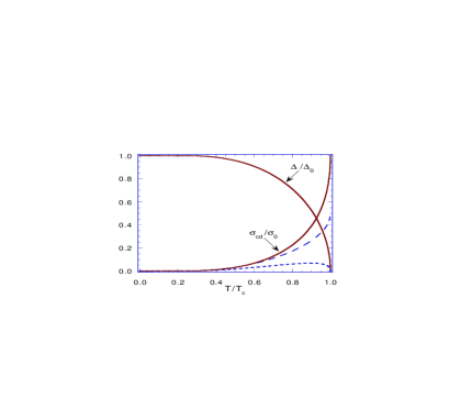
FIG. 1.: Ratio of the BCS model condensate drag conductivity $\sigma_{cd}=\sigma^{qp}_{ee}+\sigma^{qp}_{hh}+2\sigma^{qp}_{eh}=\rho_{cd}^{-1}$ to the normal double layer conductivity $\sigma_{0}$ as a function of $T/T_{c}$ for $m_{e}=m_{h}$ and $\tau_{ne}=\tau_{nh}$. Also plotted: quasiparticle conductivities $\sigma^{qp}_{ee}/\sigma_{0}$ (long-dashed line), and $-\sigma^{qp}_{eh}/\sigma_{0}$ (short dashed line), and BCS gap $\Delta$ in units of its zero temperature value $\Delta_{0}$.

REFERENCES

• [1] S.I. Shevchenko, Fiz. Nizk. Temp. 2, 505 (1976) [Sov. J. Low Temp. Phys. 2, 251 (1976)]; Yu. E. Lozovik and V.I. Yudson, Pis’ma Zh. Eksp. Teor. Fiz. 22 556 (1975) [JETP Lett. 22, 271 (1975)]; ibid, Zh. Eksp. Teor. Fiz. 71, 738 (1976) [Sov. Phys. JETP 44, 389 (1976)].
• [2] T. Fukuzawa, E.E. Mendez, and J.M. Hong, Phys. Rev. Lett. 64, 3066 (1990).
• [3] J.A. Kash, M. Zachau, E. Mendez, J.M. Hong, and T. Fukuzawa, Phys. Rev. Lett. 66, 2247 (1991).
• [4] U. Sivan, P.M. Solomon, and H. Shtrikman, Phys. Rev. Lett. 68, 1196 (1992).
• [5] B.E. Kane, J.P. Eisenstein, W. Wegscheider, L.N. Pfeiffer, and K.W. West, Appl. Phys. Lett. 65, 3266 (1994).
• [6] Y. Kuramoto and C. Horie, Solid State Commun. 25, 713 (1979); I.V. Lerner, and Yu. E. Lozovik, Zh. Eksp. Teor. Fiz. 80, 1488 (1981) [Sov. Phys. JETP 53, 763 (1981)]; Y.A. Bychkov and E.I. Rashba, Solid State Commun. 48, 399 (1983); D. Paquet, T.M. Rice, and K. Ueda, Phys. Rev. B 32, 5208 (1985).
• [7] At strong fields there is an exact mapping between electron-electron and electron-hole double-layer systems: A.H. MacDonald and E.H. Rezayi, Phys. Rev. B 42, 3224 (1990). The excitonic condensate state of the electron-hole system maps to a state with $XY$ pseudospin ferromagnetism in the electron-electron system. The Kosterlitz-Thouless transition temperature for this phase has been estimated to be as large as $\sim 0.5K$: K. Moon et al., Phys. Rev. B 51, 5138 (1995). For a review of broken symmetries of electron-electron double-layer systems in strong magnetic fields see S.M. Girvin and A.H. MacDonald in Novel Quantum Liquids in Low-Dimensional Semiconductor Structures, edited by S. Das Sarma and Aron Pinczuk (Wiley, New York, 1995).
• [8] M.B. Pogrebinskii, Fiz. Tekh. Poluprovodn. 11, 637 (1977) [Sov. Phys. Semicond. 11, 372 (1977)]; Peter J. Price, Physica 117 & 118B, 750 (1983).
• [9] H.C. Tso, P. Vasilopolous, and F.M. Peeters, Phys. Rev. Lett. 68, 1196 (1992); A.-P. Jauho and H. Smith, Phys. Rev. B 47, 4420 (1993); Lian Zheng and A.H. MacDonald, Phys. Rev. B 48, 8203 (1993); Karsten Flensberg and Ben Yu-Kuang, Hu, Phys. Rev. Lett. 73, 3572 (1994); Karsten Flensberg, B. Y. -K Hu, A. -P. Jahuo, and J. M. Kinaret, preprint (cond-mat 950409-2) 1995; Alex Kamenev and Yuval Oreg, Phys. Rev. B 52, 7516 (1995); Martin Bonsager and A.-P. Jauho, preprint (1995); L. Swierkowski, J. Szymanski, and Z. W. Gortel, Phys Rev. Lett 74, 3245 (1995); E. Shimshoni and S. L. Sondhi, Phys. Rev. B 49 11484 (1994).
• [10] T.J. Gramila, J. P. Eisenstein, A.H. MacDonald, L.N. Pfeiffer, and K.W. West, Phys. Rev. Lett. 66, 1216 (1991); T.J. Gramila, J.P. Eisenstein, A.H. MacDonald, L.N. Pfeiffer, and K.W. West, Surface Sci., 263, 446 (1992); T.J. Gramila, J.P. Eisenstein, A.H. MacDonald, L.N. Pfeiffer, and K.W. West, Phys. Rev. B 47, 12957 (1993). See also P.M. Solomon, P.J. Price, D.J. Frank, and D.C. La Tulipe, Phys. Rev. Lett. 63, 2508 (1989).
• [11] S. R. DeGroot and P. Mazur Non-equilibrium thermodynamics, (Dover Publications, Inc. New York 1962); Chapt. 5; I. Prigogine, Introduction to Thermodynamics of Irreversible Processes (Wiley, New York, 1961).
• [12] See for example Michael Tinkham, Introduction to Superconductivity, (McGraw-Hill, New York, 1975); P.G. DeGennes Superconductivity of Metals and Alloys, (Benjamin, New York, 1966).
• [13] In our calculation we assume that BCS theory is approximately valid for electron-hole systems but treat the effective interation which enters the theory, which is difficult to determine reliably, as a phenomenological parameter.
• [14] G. D. Mahan, Many-particle physics, (Plenum Press, New York 1990); Chapter 9.
Refer to caption