Integrability and Applications of the Exactly-Solvable Haldane-Shastry One-Dimensional Quantum Spin Chain

Integrability and Applications of the Exactly-Solvable Haldane-Shastry One-Dimensional Quantum Spin Chain
Johan Cornelis Talstra

A dissertation

presented to the faculty

of Princeton University

in candidacy for the degree

of Doctor of Philosophy

Recommended for acceptance

by the department of Physics

November 1995

© Copyright 1995 by Johan Cornelis Talstra.
All rights reserved.

Abstract

Recently, the one dimensional model of $N$ spins with $S=\frac{1}{2}$ on a circle, interacting with an exchange that falls off with the inverse square of the separation:
$H_{\rm ISE}=\sum_{i\neq j}\frac{1}{[\frac{N}{\pi}\sin(\frac{i-j}{N}\pi)]^{2}}({\bf S}_{i}\cdot{\bf S}_{j}-\frac{1}{4})$, or ISE-model, has received ample attention. This model was introduced by Haldane and Shastry in 1988. Its special features include: relatively simple eigenfunctions, non-interacting elementary excitations that obey semionic statistics (spinons), and a large “quantum group” symmetry algebra called the Yangian. This model is fully integrable, albeit in a slightly different sense than the more traditional nearest neighbor exchange (NNE) Heisenberg chain. The simplicity of the ISE-model warrants its paradigmatic rôle as the semionic analog of the free boson or fermion gas.

This thesis comes in two parts. Part I (chapters 1 and 2) deals with the integrability of the model, and Part II (chapters 3 and 4) discusses some of its applications. Chapter 1 introduces the model and presents the construction of a subset of the eigenfunctions. The other eigenfunctions are shown to be generated by the action of the Yangian symmetry algebra of $H_{\rm ISE}$. The Yangian is derived from a transfer matrix, thus establishing a relation to more common exactly solvable models. Chapter 2 presents a method to construct the set of constants of the motion of the ISE-model. Normally they derive from the trace of transfer matrix, but here they are obtained by considering the deformation of the spin model into a dynamical version.

The ISE-model is tractable enough to obtain its zero-magnetic-field dynamical structure factors. Chapter 3 attempts to extend this to a non-zero magnetic field, where, due to the presence of spinons in the groundstate, more complicated excitations contribute: in low fields just up to two extra spinons, for high fields two oppositely moving magnons. We discuss the relation to the more complicated NNE-model. Finally chapter 4 illustrates how a recently conjectured new form of Off Diagonal Long Range Order in antiferromagnetic spin chains can be reinterpreted as a spinon propagator in the ISE-model, and verified numerically. We briefly comment on its relevance to stabilizing superconductivity in the layered cuprates.

Acknowledgements

It is a great pleasure to thank my advisor, Duncan Haldane, for sharing his enthusiasm, his many ideas and his insights with me, and for making available the means to follow up on these. I want to thank Steve Strong for the great time we had collaborating, of which Chapter 4 of this thesis is hopefully a testimony.

I also benefited greatly from the interaction with the other graduate students and faculty at Princeton. I acknowledge very useful comments from a non-condensed matter perspective from Prof. Curt Callen. I want to thank Zach Ha and Chetan Nayak for discussions, and I mention Eddy van de Wetering, since it is partially his example that brought me to Princeton. I especially thank Per Kraus, for making our office a place to learn and to relax, scientifically and otherwise.

Finally, for many months of hospitality throughout the last 5 years as well as constant parental encouragement and support, I am deeply indebted to my family.

While at Princeton, I was supported by teaching assistantships from the University, an IBM Graduate Fellowship, and lastly by NSF grant # DMR 9224077.

To my parents

Preface

The work in this thesis is all based on previously published work. Chapter 1 is an extension of work started in Phys. Rev. Lett. 69, 2021 (1992), by F.D.M. Haldane, Zach Ha, J.C. Talstra, Denis Bernard and Vincent Pasquier. Chapter 2 was done in collaboration with Duncan Haldane and is reported in J. Phys. A. Math. Gen. 28, 2369 (1995). Chapter 3 on structure functions, also in collaboration with Duncan Haldane, appeared in Phys. Rev. B 50, 6889 (1994). Chapter 4 grew out of work with Steve Strong and Phil Anderson. It has appeared in Phys. Rev. Lett. 74, 5256 (1995).

Chapter Introduction

In this thesis, we will confine ourselves almost exclusively to one space dimension, and mostly one specific model that hasn’t been realized experimentally yet. The experimental side of other models that we will discuss is going to receive little attention either. Given these serious restrictions, one may wonder to what extent this work should belong to the field of Condensed Matter Physics. We will try to address this concern in three steps.

Why one dimensional physics? The fabulous thing about one dimensional Quantum Mechanics (or equivalently two dimensional statistical mechanics) is that there exist interacting many-particle models that are exactly solvable. Unlike in higher dimensions, particles cannot evade each other and have to scatter. For special choices of the interaction potential, particles can be made to propagate in plane waves between scattering events. During a collision they exchange their plane wave momenta. The coefficients of both sets of plane waves (before and after) are related to each other by the phase shift, picked up by the two particles that scattered. This heuristic attempt at formulating a wavefunction is called the Bethe Ansatz [Suth85, B31]. The Bose gas with delta-function interactions is an example where the Ansatz works.

We use the word solvability in the sense that the corresponding Schrödinger differential/difference equation can be reduced to a system of algebraic equations that can be solved, at least numerically . For most models the latter is indeed all one can do analytically. This brings us to the second point: why we discuss one specific model, viz. the model with $N$ spin-$\frac{1}{2}$ particles distributed equidistantly on a circle, coupled with an exchange interaction that decays proportional to the inverse squared distance between the spins:

$$H_{\rm ISE}=\sum_{i\neq j}^{N}\frac{1}{\left[(\frac{N}{\pi})^{2}\sin(\frac{i-j}{N}\pi)\right]^{2}}{\bf S}_{i}\cdot{\bf S}_{j}.$$

It is also called the Inverse Square Exchange or ISE-model. In this model solvability means a great deal more: not only are a lot of the physically relevant eigenstates known analytically (and the others can be generated via the action of ladder operators), they are also of a relatively simple form, so one can actually calculate things like structure factors in closed form. These are averages of local operators in a certain state. To date this is still impossible in the Bethe Ansatz style models.

The benefits don’t stop here; the elementary excitations of this model, so-called spinons, are spin-$\frac{1}{2}$ particles that obey semion statistics, that is to say, for every two spinons we create, there is one less orbital available for the next spinon. For fermions this would be 2 and for bosons this would be 0. This is an example of the exclusion statistics interpretation of fractional statistics [H91b], as opposed to the usual exchange statistics of the two dimensional fractional quantum hall effect (in which case both formulations can be shown to be consistent). The long range spin model is not the only place where one finds fractional excitations, but contrary to spin models such as the traditional Nearest Neighbor Exchange (NNE) Heisenberg model, the ISE-model describes a free gas of these spinons.

In the continuum limit there exists another solvable interacting model, the Sutherland model [Suth71], of $M$ bosonic particles on a circle of circumference $N$, repelling each other via a $\frac{1}{r^{2}}$ interaction, which has fractional excitations.

$$H_{\rm Suth}=-\sum_{i}^{M}\partial^{2}_{x_{i}}+\lambda(\lambda-1)\sum_{i\neq j}^{M}\frac{1}{\left[(\frac{N}{\pi}\sin(\frac{x_{i}-x_{j}}{N}\pi)\right]^{2}}$$

As a matter of fact, one can select their statistics, by varying the coupling constant in the potential energy. For a particular value of that coupling $\lambda=2$, (corresponding to exactly semion statistics) we can set up a mapping to the ISE spin model. The mapping identifies a number of low lying states in the continuum with a number of maximal $S^{z}$ states in the spin model. The correspondence is not trivial in that all other (missing) spin states are obtained by the action of some simple symmetry like $SU(2)$ or $SU(2)\times SU(2)$ (as in the NNE and 1D Hubbard models respectively). Recently it was found that the “missing” states are generated by acting on the “continuum” wavefunctions with the much larger symmetry algebra called the Yangian, $Y(sl_{2})$, a quantum deformation of the $SU(2)$ Lie group. Unlike the case of the Quantum Affine Algebra extension of $SU(2)$: $U_{q}(\widehat{sl}_{2})$, the Yangian is not obtained by deforming the Lie group commutation relations, but rather by adding new generators. The Yangian algebra is well studied in the mathematics literature and was first introduced into physics in quantum field theory [B91]. The spin model is the first finite system which serves as a representation of this algebra. It can be studied in a hands-on manner, for instance on a computer, and one can construct the ladder operators explicitly, just as for SU(2) spins.

At this point we comment on the third issue: the relation to experiments. The utility of the ISE-model and its Yangian doesn’t lie so much in the fact that it clarifies experiments, waiting for an explanation, but rather, it presents a new paradigm, a language. We mean this in the same sense that free boson and fermion models are paradigms that do not occur in nature, but a class of more realistic models only differ from them by the addition of irrelevant perturbations; these models reside in the same universality class, and have essentially the the same long distance physics as the free fixed points. Similarly, the nearest neighbor Heisenberg model is in the same universality class as the ISE model, but its semions are weakly interacting, as we will see in chapter 3.

The remainder of this thesis is organized as follows. The first part, chapters 1 and 2, will be concerned with the “exactly solvable” qualifier of the ISE-model, illustrating the richness of the underlying integrability structure. Chapters 3 and 4 are more applied and stress the paradigmatic aspects of the model. Chapter 1 will review the relevant facts about the solutions of the ISE spin-model, and show how its Yangian symmetry emerges. In other words, we will try to construct the transfer matrix of this model. Chapter 2 is a bit more technical in nature. In general, all exactly solvable models will possess a set of commuting operators of which the Hamiltonian is one: the constants of the motion (in classical physics, the conserved quantities). The usual derivation of these quantities does not work for the ISE model, for the precise reason that the Yangian is an exact symmetry of the ISE Hamiltonian. By deforming the model through allowing the particles to leave their lattice sites, via a kinetic energy term, and taking the limit where the spin potential energy dominates the kinetic energy we can recover these constants of the motion.

Chapter 3 describes the dynamical correlation functions of the ISE-model in a non-zero magnetic field, where some knowledge of the underlying Yangian structure—the division of the Hilbert space into Yangian multiplets—is actually required. It builds on recent work based on various methods, such as supersymmetric matrix functional integrals [als93, hz93] and Jack polynomial techniques [Ha94] from mathematics, which obtained these structure functions (or Greens functions in the corresponding quantum field theory), exactly, at at zero external field. We investigate the case $h\neq 0$, in which case the $h$-field tunes the number of fractional quasiparticles in the groundstate.

Finally, chapter 4 show how a new order parameter for antiferromagnetic spin models [RVB] can be analyzed in the free spinon ISE-model. The order parameter involves inserting two sites into a spin chain and putting two spins in a singlet configuration on them. Whereas only numerical and circumstantial evidence exists for the Long Range Order (LRO) of this order parameter in the NNE-model, it can be approached analytically in the ISE-model, once we interpret the order parameter as a spinon propagator. Some analogies to the $\nu=\mbox{$\frac{1}{2}$}$ bosonic FQHE are drawn, and we suggest some implications for stabilizing superconductivity in layered cuprates via singlet pair hopping.

Part I Integrability Structure of the $\frac{1}{r^{2}}$-Spin model.

Chapter 1 The Inverse Square Exchange Spin Model and its Yangian.

1.1 Introduction

Solvable models play an interesting rôle in many-body physics and not just because of the mathematical satisfaction of being able to obtain the exact solution to a particular problem. In a world of uncontrolled approximations, they can be the touchstone and foundation of theories that describe “real” systems more realistically than the mathematical toy models themselves. The 1-D Hubbard model of spin-1/2 fermions on a circle illustrates this eminently [RVBbook].

Although nowadays scores of models have been solved exactly, many of them still await practical application. This is not surprising considering the mathematical tour de force that is often required. A consequence is that solving a model (i.e., knowing the eigenfunctions of that particular Hamiltonian) does not mean that we can actually compute physical properties if those wavefunctions are of a complicated nature. Such is the case for the Nearest Neighbor Exchange $S=1/2$ Heisenberg-chain, for example. Its Hamiltonian is given by [bethe31]:

$$H_{\rm NNE}=J\sum_{i=1}^{N}{\bf S}_{i}\cdot{\bf S}_{i+1},$$ (1.1)

where ${\bf S}_{N+1}={\bf S}_{1}$.

A system that doesn’t suffer from this problem is the model of spin-$\frac{1}{2}$ particles on a one-dimensional ring, interacting antiferromagnetically through an Inverse Square Exchange interaction (ISE-model for short). It was introduced in 1988 by Haldane and Shastry [H88, S88]. The Hamiltonian is as follows:

$$H_{\rm ISE} = \frac{J}{4}\sum_{i\neq j=1}^{N}d(i-j)^{-2}(P_{ij}-1)$$ (1.2)

$$= \frac{v_{s}}{\pi}\sum_{i\neq j=1}^{N}d(i-j)^{-2}({\bf S}_{i}\cdot{\bf S}_{j}-\frac{1}{4}),$$

where $P_{ij}$ permutes the spins on sites $i,j$ and $d(i-j)$ represents the chord distance between two points $i,j$ on a circle that has been subdivided into equidistant sites: $d(n)=|\frac{N}{\pi}\sin^{2}(\frac{n\pi}{N})|^{2}$. Periodic boundary conditions are assumed.

Despite the long range of the force between the spins, this model is solvable to a much larger extent than its short-ranged cousins. The key feature is the non-transcendental structure of the eigenfunctions of (1.2), and the simplicity of the spectrum. It may seem that the particular exchange integral in eq. (1.2) makes $H_{\rm ISE}$ less suited as a paradigm for a family of physically applicable models (but see [Vacek93] for exceptions). However, the fact that the model’s solution is simple, in combinations with the fractional statistics nature of the elementary excitations in its spectrum, make it an appropriate candidate for an ideal gas of anyons.

We will start with a short introduction to the ISE-model and its integrability structure; precise details can be found in [H94, BL95]. Section 1.2 will explain how $H_{\rm ISE}$ was solved originally. Section 1.3 will analyze the symmetries of the Hamiltonian and provide an explanation for the exact degeneracies of its spectrum. The methods on which section 1.3 are based, are familiar from quantum inverse scattering and the Yang-Baxter equation literature—thereby elucidating the relation to more conventional solvable models.

1.2 The ISE-Hamiltonian and its Spectrum

To solve the Schrödinger equation for $H_{\rm ISE}$ let us first transcribe it into a language of hard-core bosons on a lattice, where down-spins are considered particles and up spins represent the absence of these particles. The hard-core constraint refers to projecting out the states in the Hilbert space with more than one particle per site. With $M$ particles present, $S^{z}=\mbox{$\frac{1}{2}$}N-M$. The usual separation of the ${\bf S}_{i}\cdot{\bf S}_{j}$ term into a kinetic energy part ($S^{+}_{i}S^{-}_{j}+S^{-}_{i}S^{+}_{j}$) and a potential energy part $S^{z}_{i}S^{z}_{j}$, reduces eq. (1.2) to [Fradkin91]:

$$\sum_{k=1}^{N}\epsilon_{0}(k)\hat{\rho}_{k}+\frac{v_{s}}{\pi}\sum_{i\neq j=1}^{N}d(i-j)^{-2}n_{i}n_{j},$$ (1.3)

where the discrete Fourier transform of the exchange is $\epsilon_{0}(k)=\frac{v_{s}}{2\pi}k(k-2\pi)$, $k=\frac{2\pi}{N}m,\>m=0\ldots N-1$. $S^{-}_{j}=c^{\dagger}_{j}$, $n_{j}=c^{\dagger}_{j}c_{j}=\mbox{$\frac{1}{2}$}-S^{z}_{j}$, and $\hat{\rho}_{k}=\hat{c}^{\dagger}_{k}\hat{c}_{k}$ is the usual number operator for the extended orbital with momentum $k$. From now on we will measure energy in units of $(\frac{2\pi}{N})^{2}\frac{v_{s}}{\pi}$. Notice that the kinetic energy is strictly quadratic (albeit periodically repeated in successive Brillouin zones), despite the fact that the particles hop on a lattice. This peculiar connection with the kinetic energy in the continuum is a special property of the $1/\sin^{2}$ potential that people have attempted to employ before in the context of fermion lattice gauge theory [Drell76]. This phenomenon raises the suspicion that the relation between the lattice model and some continuum model of particles on a ring may be exploited. Haldane and Shastry [H88, S88, H91] found indeed that the set of eigenfunctions of the continuum Hamiltonian of the so-called Sutherland model [suth70]:

$$H=-\sum_{i}^{M}(\partial_{i})^{2}+\sum_{i<j}^{M}\frac{2\lambda(\lambda-1)}{(\frac{N}{\pi})^{2}\sin^{2}(\frac{x_{i}-x_{j}}{N}\pi)},$$ (1.4)

of $M$ particles on a circle of circumference $N$ are also eigenfunctions of $H_{\rm ISE}$ via the particle/down-spin analogy. Let us repeat this derivation since it involves a few transformations that we will run into frequently.

Sutherland found the (unnormalized) groundstate for his continuum model to be of the simple Jastrow form:

$$\Psi_{0}(n_{1},\ldots,n_{M})=\prod_{i<j}\left|\sin(\frac{x_{i}-x_{j}}{N}\pi)\right|^{\lambda}.$$ (1.5)

This is the case of bosons; for fermions we adopt (1.5) for $x_{1}<x_{2}\ldots<x_{M}$ and multiply with the appropriate sign for other orderings of the particles.

As a notational aside, in the spin model on the circle—with a lattice spacing that we have chosen to be 1—let us parametrize the sites with the complex numbers $\left\{z_{j}=e^{\frac{2\pi i}{N}j}\right\}_{j=0}^{N-1}$. The locations of the particles (down-spins) $\{n_{i}\}_{i=1}^{M}$ in a given spin-configuration denoted by the ket $|n_{1},n_{2},\ldots,n_{M}\rangle$, are given by ${z_{n_{j}},\>j=1,\ldots,M}$ and $0\leq n_{j}<N$. As an example, in this complex notation the “interaction potential” between down-spins becomes: $(\frac{2\pi}{N})^{2}\cdot\frac{-z_{n_{i}}z_{n_{j}}}{(z_{n_{i}}-z_{n_{j}})^{2}}$. Haldane and Shastry showed that (1.5) is an eigenstate of spin Hamiltonian (1.2) as well if we restrict the $x_{i}$ to the lattice, i.e. to be integers $\{n_{i}\}$, and pick $\lambda=2$. In other words, the spin groundstate is a member of the family of wavefunctions (in complex notation):

$$\psi_{0}(z_{n_{1}},\ldots,z_{n_{M}})=\prod_{i<j}^{M}(z_{n_{i}}-z_{n_{j}})^{2}\prod_{i=1}^{M}z_{n_{i}}^{J}=\prod_{i<j}\sin^{2}(\frac{n_{i}-n_{j}}{N}\pi)\prod_{i}e^{\frac{2\pi i}{N}(J+2(M-1))n_{i}}.$$ (1.6)

In the spin model, the absolute groundstate as function of $M$ occurs when $J=1,\,M=N/2$, and $S^{z}=0$, (at least for $N$ even, which is what we will assume in the rest of this chapter). In the sector $M\neq\frac{N}{2}$ we have to choose $J=1+\frac{N}{2}-M$ to find the state with lowest energy for that value of $S^{z}$. For what follows we choose $J=1$. Here, and in the following we adhere to the convention that uppercase greek letters refer to wavefunction of the $\{n_{i}\}$ and lowercase greek letters to functions of the $\{z_{n_{i}}\}$. That is: $\Psi_{0}$ is related to $\psi_{0}$ as follows:

$$\Psi_{0}(n_{1},\ldots,n_{M})\equiv\psi_{0}(z_{n_{1}},\ldots,z_{n_{M}}).$$ (1.7)

As we shall see in section 1.2.2, the excited states in the continuum are obtained by multiplying the groundstate wavefunction by a symmetric set of plane-wavefunctions—$\Psi=\Psi_{0}(x_{1}\ldots x_{M})\Phi(x_{1}\dots x_{M})$, with momenta that satisfy simple Bethe-Ansatz type equations. The rationale is that the strong correlations are described well by the “groundstate” wavefunction and small fluctuations are added by the multiplying factor. In the spin case we can try the same: we write a spin wavefunction as the product of the wavefunction (1.6) and some symmetric polynomial $\phi$ in the ${z_{n_{i}}}$:  $\Psi(n_{1},\ldots,n_{M})=\Psi_{0}(n_{1},\ldots,n_{M})\Phi(n_{1},\ldots,n_{M})$. The crux the mapping of $H_{\rm ISE}$ onto the continuum Sutherland Hamiltonian is the following: the spin Schrödinger equation for $\Psi_{0}\Phi$ which is really a difference equation for $\Phi$, can be rewritten as a differential equation in $\Phi$, if the latter is of a polynomial (i.e. plane wave) form. This differential equation is identical to the continuum Schrödinger equation that $\Phi(x_{1}\ldots x_{M})=\frac{\Psi^{\rm cont}(x_{1}\ldots x_{M})}{\Psi^{\rm cont}_{0}(x_{1}\ldots x_{M})}$ satisfies (the superscript “cont” indicates that the $x_{i}$ are considered continuum variables). This equation has been solved in [suth70]. Let us first illustrate the difference-to-differential transformation.

1.2.1 From the Lattice to the Continuum

In complex notation:

$$H_{\rm ISE}=H_{1}+H_{2}=\sum_{i\neq j}\frac{-z_{i}z_{j}}{(z_{i}-z_{j})^{2}}S^{z}_{i}S^{z}_{j}+\sum_{i\neq j}\frac{-z_{i}z_{j}}{(z_{i}-z_{j})^{2}}\mbox{$\frac{1}{2}$}(S^{+}_{i}S^{-}_{j}+S^{-}_{i}S^{+}_{j})$$ (1.8)

We have dropped the additive constant part in $H_{\rm ISE}$ for now, and we will put it back in at the end, by requiring that the fully polarized state $|\uparrow\cdots\uparrow\rangle$ has zero energy. Now $\langle n_{1},\ldots,n_{M}|H_{1}|\Phi\Psi_{0}\rangle=\Phi(n_{1},\ldots,n_{M})\langle n_{1},\ldots,n_{M}|H_{1}|\Psi_{0}\rangle$ since $H_{1}$ is diagonal in the particle number occupation basis. Furthermore

$$\langle n_{1},\ldots,n_{M}| H_{2} |\Phi\Psi_{0}\rangle=\sum_{j=1}^{M}\sum_{i\neq n_{j}}^{N}-\frac{z_{i}z_{n_{j}}}{(z_{i}-z_{n_{j}})^{2}}\times$$ (1.9)

$$\Psi_{0}(n_{1},\ldots,n_{j-1},i,n_{j+1},\ldots)\Phi(n_{1},\ldots,n_{j-1},i,n_{j+1},\ldots).$$

We can write this as a “continuum” expression with the help of the fact that the Fourier transform of $1/\sin^{2}$ is quadratic:

$$\sum_{n(\neq m)}^{N}\frac{z_{n}z_{m}}{(z_{n}-z_{m})^{2}}P(z_{n})=\left\{-\mbox{$\frac{1}{2}$}(z_{m}\partial_{z_{m}})^{2}+\frac{N}{2}z_{m}\partial_{z_{m}}-\frac{1}{12}(N^{2}-1)\right\}P(z_{m})$$ (1.10)

if $P(z)$ is a polynomial of degree $<N$ in every variable. Since $\psi_{0}$ is of has powers of $z_{n_{i}}$ in the range $0,\ldots,2(M-1)+1$, this means that we can only apply eq. (1.10) if $\phi$ has a degree in the range $0,\ldots,N-2M$ in all its entries. This somewhat arbitrary constraint from the point of view of the spin model will become clearer later on. Then, with the Leibnitz rule for differentiation: the $H_{2}$ matrix elements (1.9) become,

$$-\Phi(n_{1},\ldots,n_{M})\left(\sum_{j=1}^{M}\left[-\frac{1}{12}(N^{2}-1)+\frac{N}{2}(z_{n_{j}}\partial_{n_{j}})-\mbox{$\frac{1}{2}$}(z_{n_{j}}\partial_{n_{j}})^{2}\right]\psi_{0}\right)$$

$$+-\sum_{j=1}^{M}\left(-\mbox{$\frac{1}{2}$}\cdot 2\cdot\left[(z_{n_{j}}\partial_{n_{j}})\psi_{0}\right]+\frac{N}{2}\psi_{0}-\mbox{$\frac{1}{2}$}\psi_{0}(z_{n_{j}}\partial_{n_{j}})\right)(z_{n_{j}}\partial_{n_{j}})\phi$$

$$\equiv\Phi(n_{1},\ldots,n_{M})\langle n_{1},\ldots,n_{M}|H_{2}|\Psi_{0}\rangle+\Psi_{0}(n_{1},\ldots,n_{M})\langle n_{1},\ldots,n_{M}|H_{2}^{\prime}|\Phi\rangle$$

where $H_{2}^{\prime}=\sum_{j=1}^{M}\mbox{$\frac{1}{2}$}(z_{n_{j}}\partial_{n_{j}})^{2}+\sum_{j\neq k}^{M}w_{n_{j}n_{k}}z_{n_{j}}\partial_{n_{j}}-{\rm deg}(\Phi)(\frac{N}{2}-M)$. $w_{ij}=\frac{z_{i}+z_{j}}{z_{i}-z_{j}}=-i\cot(\frac{i-j}{N}\pi)$. Remember that $\phi$ is a symmetric polynomial and therefore homogeneous of degree ${\rm deg}(\phi)$ and satisfies Euler’s theorem. Now using the Schrödinger equation: $H(\Psi_{0}\Phi)=E\cdot(\Phi\Psi_{0})$ and $H\Psi_{0}=E_{0}(M)\Psi_{0}$, we have $H_{2}^{\prime}\Phi=(E-E_{0}(M))\Phi$. This reduced Schrödinger equation for $\Phi$ is identical to the equation obtained when $\Psi_{0}\cdot\Phi$ would have been considered a continuum expression and be plugged into the continuum limit Schrödinger equation (1.4), provided $\lambda=2$ [suth70]. For good measure: $E_{0}(M)=\frac{1}{6}M(4M^{2}-1)-\mbox{$\frac{1}{2}$}M^{2}N$. The case $\lambda\neq 2$ would correspond to an XXZ generalization of the isotropic spin model. We follow the solution of Sutherland for diagonalizing $H_{2}^{\prime}$ in the next section.

1.2.2 Eigenstates of the Sutherland Hamiltonian

The (non-hermitean) Schrödinger equation for $\Phi$ can be solved by choosing a basis in the space of the symmetric polynomials, such that $H_{2}^{\prime}$ becomes triangular. The eigenvalues can then be read off from the diagonal. The obvious basis for symmetric polynomials are the functions $\phi^{|m|}=\sum_{P\in S_{M}}\prod_{i=1}^{M}z_{n_{i}}^{m_{P(i)}}$, where $0\leq m_{1}\leq\ldots\leq m_{M}\leq N-2M$. Notice: ${\rm deg}(\phi^{|m|})=\sum_{i}m_{i}$. The only degree of freedom left to make $H_{2}^{\prime}$ triangular is to order the different partitions $|m|$. The off-diagonal action of $H_{2}^{\prime}$ on a basis state $\phi^{|m|}$ is to produce a linear combination of other basis states that are labeled by partitions obtained from repeatedly “squeezing” partition $|m|$ [suth70]. We say that $|n|$ is produced by squeezing $|m|$ if $m_{k}=n_{k},k\neq i,j$ and if for some $i<j$: $n_{i}=m_{i}+1$, $n_{j}=m_{j}-1$. This is illustrated in the next figure:

$$\begin{array}[]{ccccc}m_{1}&m_{2}&m_{3}&m_{4}&m_{5}\\ 1&3&4&6&9\\ &\rule{8.00003pt}{0.0pt}\uparrow_{+1}&&\rule{8.00003pt}{0.0pt}\uparrow_{-1}&\\ \end{array}\rule{20.00003pt}{0.0pt}\Longrightarrow\rule{20.00003pt}{0.0pt}\begin{array}[]{ccccc}n_{1}&n_{2}&n_{3}&n_{4}&n_{5}\\ 1&4&4&5&9\\ &&&&\end{array}$$

Thus, if we order the states according to whether they can or cannot obtained from each other by repeatedly squeezing, $H_{2}^{\prime}$ is by definition diagonal. This is possible since this partial ordering is transitive. The eigenfunctions of $H_{2}^{\prime}$ are then labeled by a unique partition $|m|$ and consist of a linear combination of the corresponding basis state plus all its squeezed descendants. They are known in the mathematics literature as Jack polynomials [forrester93, stanley90, zncha94]. The energy of such a state is then [suth70]:

$$E_{0}(M)+\mbox{$\frac{1}{2}$}\{\sum_{j}(n_{j}^{2}-2(M+1-2j)n_{j}\}-(\frac{N}{2}-M)\sum_{j}n_{j}=\mbox{$\frac{1}{2}$}\sum_{j=1}^{M}m_{j}(m_{j}-N),$$ (1.12)

where the $m_{j}=n_{j}+2j-1$ are a more convenient set of variables in the range $0<m_{j}<N$. These variables, which are distinct and cannot be consecutive either, are called pseudomomenta. The ${m_{j}}$ satisfy an equation that makes contact with Asymptotic Bethe Ansatz methods:

$$e^{\frac{2\pi i}{N}m_{i}\cdot N}=\prod_{i<j}e^{\Theta(m_{i}-m_{j})}$$ (1.13)

and $\Theta(m_{i}-m_{j})=\pi{\rm sgn}(m_{i}-m_{j})$. $\Theta(m)$ is the quantum mechanical phase shift for a scattering process of two particles, with relative momentum $\frac{2\pi m}{N}$, that interact via a $\lambda(\lambda-1)/\sin^{2}(x)$ potential, at $\lambda=2$.

1.2.3 Missing States and their Origin

The states we have found thus far are all at the top of their spin multiplets: $S=S^{z}$, which can be seen easily from the fact that $\psi_{0}$ is a polynomial which vanishes at $z_{i}=0$ (see Appendix A). By acting with $S^{-}$ we can recover the rest. This gives us a total of (for $N$ even) $\left(\rule{0.0pt}{8.00003pt}^{N-M}_{\rule{4.20004pt}{0.0pt}N}\right)$ spin-multiplets with $S=\frac{N-2M}{2}$ (we have to choose $M$ $n_{k}$’s in the range ${0,\ldots,N-2M}$). We know that there ought to be $\left(\rule{0.0pt}{8.00003pt}^{N}_{M}\right)-\left(\rule{0.0pt}{8.00003pt}^{\rule{4.20004pt}{0.0pt}N}_{M-1}\right)>\left(\rule{0.0pt}{8.00003pt}^{N-M}_{\rule{4.20004pt}{0.0pt}N}\right)$ [bloch29], and the missing multiplets must be of non-polynomial form, that is, they correspond to continuum eigenfunctions with support beyond the first Brillouin zône [suth88], which gets mapped back to $[-\pi,\pi]$ because of Umklapp processes in the lattice case. Thus the trick (1.10) ceases to be valid.

However, by diagonalizing small systems numerically, Haldane [H88] finds that all these “missing” states have energies already contained in the set of energies of polynomial-type states. I.e., the energy levels have enormous degeneracies beyond the regular $SU(2)$ symmetry of the model (see table 1.1 later on). This hints at the fact that there exists some hidden symmetry generated by operators commuting with the Hamiltonian (but not amongst each other). Since the introduction of the model various operators that commute with $H_{\rm ISE}$ were suggested by Inozemtsev [Inoz90], but not with the intention of reproducing the degeneracies—all these operators commuted amongst themselves. Such an algebra should not commute with the $SU(2)$ Casimir ${\bf S}^{2}$. The two Inozemtsev invariants of the third order can be linearly combined into an operator that commutes with ${\bf S}^{2}$:

$$H_{3}=\sum_{ijk}\rule{0.0pt}{5.59721pt}^{{}^{\prime}}\frac{z_{i}z_{j}z_{k}}{z_{ij}z_{jk}z_{ki}}{\bf S}_{i}\cdot{\bf S}_{j}\times{\bf S}_{k}$$ (1.14)

where $z_{ij}=z_{i}-z_{j}$ and the sum $\sum\rule{0.0pt}{5.59721pt}^{{}^{\prime}}$ excludes terms where any of the dummy indices coincide. We will revisit this operator in chapter 2. The other linear combination:

$$I_{3}^{\prime} = \sum_{ijk}\rule{0.0pt}{5.59721pt}^{{}^{\prime}}(w_{ij}+w_{jk}+w_{ki}){\bf S}_{i}\cdot{\bf S}_{j}\times{\bf S}_{k}$$ (1.15)

$$\propto {\bf S}\cdot\left(\sum_{i\neq j}w_{ij}{\bf S}_{i}\times{\bf S}_{j}\right)\equiv{\bf S}\cdot{\bf\Lambda}$$

also commutes with ${\bf S}$ and with $H_{\rm ISE}$, but ${\bf\Lambda}$ only commutes with $H_{\rm ISE}$ and doesn’t commute with ${\bf S}^{2}$! ${\bf\Lambda}$ is called the rapidity operator, since $\Lambda^{z}$ measures the total rapidity of one of the polynomial type eigenstates, i.e., $\sum_{j}m_{j}$ (not to be confused with the translation/momentum operator which determines $\prod_{j}e^{\frac{2\pi i}{N}m_{j}}$ or $\sum_{j}m_{j}\,\,{\rm mod}\,N$). Now in Bethe’s traditional model with nearest neighbor exchange (NNE) interaction this operator has an analogue: ${\bf\Lambda}_{\rm NNE}=\sum_{i\neq j}\theta(i-j){\bf S}_{i}\times{\bf S}_{j}$, where $\theta(n)$ is the Heavyside step function = $\lim_{\kappa\rightarrow\infty}\coth(\kappa(i-j))$. So the NNE rapidity operator is seen to be a particular limit of the analytic (hyperbolic) continuation of the one in the trigonometric model with ISE, i.e., $z_{j}=e^{\frac{2\pi i}{N}j}\rightarrow e^{\kappa j}$.

The algebra generated by ${\bf S}_{\rm Tot}$ and ${\bf\Lambda}_{\rm NNE}$ has been studied in the mathematics literature and is known as a representation of the Yangian algebra $Y(sl_{2})$ ($sl_{2}$ is isomorphic to $su_{2}$). The Yangian, a Hopf algebra, was introduced in 1985 by Drinfel’d [drinfeld85] in the context of the Yang-Baxter equation (YBE), and its representation theory has been worked out subsequently by Tarasov, Kulish et al. [tarasov85] and Chari and Pressley [CP1990]. The set of Yangian operators does not commute with the Hamiltonian in the NNE model, except when $N\rightarrow\infty$. However in the long-range spin model ${\bf S}$ and ${\bf\Lambda}_{\rm ISE}$ do commute with $H_{\rm ISE}$ for any finite $N$. The entire representation of the Yangian that they generate in this case must also commute with $H$, i.e., for the ISE case $Y(sl_{2})$ is a genuine symmetry, giving rise to additional degeneracies. In other words: this particular spin model is a reducible representation of the Yangian! From the Yangian representation theory we can also understand the special rôle of the polynomial wavefunctions: they are the Yangian Highest Weight States (YHWS) of different irreducible Yangian representations. Every one of them generates an irreducible representation space by letting ${\bf S}$ and ${\bf\Lambda}$ act on them repeatedly. All the resulting states will have the same energy as their parent state, but won’t in general be polynomials.

Every irreducible $SU(2)$ representation is parametrized by one integer, since there is only one element in the Cartan algebra—for $SU(N)$ there are $N-1$ integers. For $Y(sl_{2})$ we characterize each irrep with a polynomial, the so-called Drinfel’d polynomial (a polynomial is determined by the prefactor of the highest power and the positions of its roots; here we only care about the relative positions of the roots). In the spin-chain case the degree of this polynomial is $N-2M$ for a YHWS with $M$ down-spins. The locations of its roots, which are spaced by integer multiples of some unit called $h$, are determined by the pseudomomenta $\{m_{i}\}_{i=1}^{M}$ and vice versa.

One of the things the representation theory of the Yangian algebra can teach us is the degeneracy of the multiplets: i.e., exactly which spin-multiplets occur in a given irrep, belonging to a particular energy level. Haldane [H91] has identified a rule that gives the spin-content of a particular energy level, but in the next section, we will go through the “Yangian derivation” [BGHP93, BPS93]. We will do this by constructing another irreducible representation in a Hilbert space of which we know the $SU(2)$ spin content in section 1.5.1. This representation is equivalent to one based on one of the polynomial states, as they are made to have the same Drinfel’d polynomial.

In order to understand the representation theory we should first discuss the abstract algebraic structure underlying the Yangian, the transfer matrix and the Yang-Baxter equation, in 1.4. In the case of the NNE-model the NNE representation of the transfer matrix (which contains ${\bf S}_{\rm Tot}$, ${\bf\Lambda}_{\rm NNE}$ and all other elements of the Yangian as coefficients in a power series) emerges naturally if one calculates its partition function ${\rm Tr}(e^{-\beta H})$. We construct it specifically in 1.5, as well as for the ISE-model. The transfer matrix for the latter, unfortunately doesn’t have such a nice physical interpretation, but its representation is reducible, explaining the multiplet structure of $H_{\rm ISE}$.

1.3 The Transfer Matrix, its Yangian, and the Algebraic Bethe Ansatz

Historically the Yangian emerged from a study of the algebra of the transfer matrix. Almost all exactly solvable 1D models owe their integrability to the existence of a transfer matrix which encodes the consistency rules on scattering processes that lead to the Bethe Ansatz equations [suth85]. The transfer matrix ${\bf T}(u)$ is an operator-valued matrix function of a spectral parameter $u$. $u\in\mbox{\double C}$ and ${\bf T}$ is a $2\times 2$ matrix in our $SU(2)$ case (for $SU(N):\;N\times N$). Its $n$th Taylor-expansion coefficients in $\frac{1}{u}$ contains essentially the operators generated by commuting $n$ ${\bf S}$’s and ${\bf\Lambda}$’s with each other. Specific to $SU(2)$ the transfer matrix is defined by

$$T^{ab}(u) = \sum_{\mu=0}^{3}\sigma^{ab}_{\mu}T^{\mu}(u)$$ (1.16)

$$= \delta^{ab}+\sum_{n=0}^{\infty}\frac{1}{u^{n+1}}\sum_{\mu=0}^{3}\sigma^{ab}_{\mu}J_{n}^{\mu},\,\,\,\,a,b=1,2$$

$\{\sigma_{1},\sigma_{2},\sigma_{3}\}$, the three Pauli matrices, and $\sigma_{0}=\mbox{1l}$, satisfy ${\rm Tr}(\sigma_{\alpha}\sigma_{\beta})=2\delta_{\alpha\beta}$. These Pauli matrices do not act on the local spins, but are just a convenient way to label different linear combinations of the four components of ${\bf T}$. The $J^{\mu}_{n}$ are abstract operators, but in the spin-chain representation they are combinations of the local ${\bf S}_{i}$. To follow the upcoming discussion it may be helpful to take the following into account:

$${\bf J}_{0}={\bf S}_{\rm Tot}$$

$${\bf J}_{1}\propto{\bf\Lambda}$$ (1.17)

The Yangian defining commutation relations—the algebra of ${\bf S}_{\rm Tot}$ and ${\bf\Lambda}$ and the operators generated by commuting these with each other—are encoded in the Fundamental Commutation Relations (FCR) for ${\bf T}$:

$$R(u-v)(\mbox{1l}\otimes{\bf T}(u))({\bf T}(v)\otimes\mbox{1l})=({\bf T}(v)\otimes\mbox{1l})(\mbox{1l}\otimes{\bf T}(u))R(u-v)$$ (1.18)

where $R$ is a 4x4 matrix acting on the $a,b$ indices of both ${\bf T}$’s but not in the space in which their matrix elements act, ie $R$ commutes with the $J^{\mu}_{n}$. Here $R$ is Yang’s “rational” solution (whence the name Yangian) of the Yang-Baxter equation:

$$R=u\mbox{1l}+hP_{12}.$$ (1.19)

$P_{12}$ is the operator that permutes vectors in the tensor product $\mbox{\double C}^{2}\otimes\mbox{\double C}^{2}$: $P_{12}(x\otimes y)=y\otimes x$. $h$ is some complex number, called the quantum parameter, which is fixed for a particular model. For the ISE-model, the Drinfel’d polynomial will turn out to have real roots, and we can normalize $h$ to 1. For the NNE-model, complex roots occur in a pattern symmetric around the imaginary axis, and it is customary to choose $h=i$. From now on we will use the summation convention with a sum over Greek indices running from $0\ldots 3$ and Latin indices running from $1\ldots 3$. The FCR (1.18) can be written out more transparently in components:

$$(u-v)[T^{ab}(u),T^{cd}(v)]=h(T^{cb}(v)T^{ad}(u)-T^{cb}(u)T^{ad}(v))$$ (1.20)

This holds in general for a chain based on for $sl_{n}$ spins as well. Notice that for $h\rightarrow 0$ the transfer matrix commutes with itself; this is referred to as the classical limit. For the particular case of a spin-$\frac{1}{2}$ model we rewrite (1.20) in basis of $\sigma$-matrices:

$$\begin{array}[]{rclr}(u-v)[T^{0}(u),T^{i}(v)]&=&\frac{h}{2}i\epsilon_{ijk}T^{j}(v),T^{k}(u)\},&(a)\\ (u-v)[T^{i}(u),T^{j}(v)]&=&\frac{h}{2}i\epsilon_{ijk}(T^{k}(v)T^{0}(u)-T^{k}(u)T^{0}(v))&(b)\\ &=&\frac{h}{2}i\epsilon_{ijk}(\{T^{0}(u)T^{k}(v)-T^{0}(v)T^{k}(u))&\end{array}$$ (1.21)

$\{,\}$ denotes the anticommutator. Expanded in modes this becomes:

$$\begin{array}[]{rclr}\left[J^{0}_{m+1},J^{i}_{n}\right]-\left[J^{0}_{m},J^{i}_{n+1}\right]&=&\frac{h}{2}i\epsilon_{ijk}\{J^{j}_{n},J^{k}_{m}\}&(a)\\ \left[J^{i}_{m+1},J^{j}_{n}\right]-\left[J^{i}_{m},J^{j}_{n+1}\right]&=&\frac{h}{1}i\epsilon_{ijk}(J^{k}_{n}J^{0}_{m}-J^{k}_{m}J^{0}_{n})&(b)\\ &=&\frac{h}{2}i\epsilon_{ijk}(J^{0}_{m}J^{k}_{n}-J^{0}_{n}J^{k}_{m})&\end{array}$$ (1.22)

This is to be supplied with the “boundary condition” $J^{0}_{-1}=\mbox{1l}$; ${\bf J}_{-1}=0$. In deriving (1.21, 1.22) we have used the fact that $[T^{\mu}(u),T^{\nu}(v)]=[T^{\mu}(v),T^{\nu}(u)]$, which follows from adding the FCR and the one with $u$ and $v$ interchanged. An important consequence of this last relation with $\mu=\nu$ is that the components of the transfer matrix commute with themselves for different values of the spectral parameter. In particular, if $\mu=\nu=0$ we have $[{\rm Tr}({\bf T}(u)),{\rm Tr}({\bf T}(v))]=0$. If we expand this result in powers of $u,v$ we find $[J^{0}_{m},J^{0}_{n}]=0$ $\forall_{m,n}$, i.e., we have a set of commuting operators. For the NNE model, the Hamiltonian is a member of this family, and thus we obtain a set of constants of motion. However $[{\rm Tr}({\bf T}),T^{ab}]\equiv 0$ only for $N\rightarrow\infty$, so the Yangian doesn’t provide any extra degeneracies. Unfortunately, for the ISE model $H_{\rm ISE}$ cannot be a member of that family since $H_{\rm ISE}$ commutes with ${\bf T}$. We will return to this issue in chapter 2.

Let us look at eq. (1.22) for a few particular cases. When we choose $m=-1$ in (1.22^a) we find: $[J^{0}_{0},{\bf J}_{n}]=0$ so $J^{0}_{0}$ commutes with the algebra and is scalar. Setting $m=-1$ in (1.22^b): $[J^{i}_{0},J^{j}_{n}]=hi\epsilon_{ijk}J^{k}_{n}$, i.e., the ${\bf J}$ are $SU(2)$ vector operators. Similarly with $m=0$ in (1.22^a) we find that the $J^{0}_{n}$ are scalars. With $m=0$ in (1.22^b) we have:

$$i\epsilon_{ijk}[J^{j}_{1},J^{k}_{n}]=-2J^{i}_{n+1}-2h(J^{0}_{0}+1)J^{i}_{n}-2hJ^{i}_{0}(J^{0}_{n}).$$ (1.23)

This last equation tells us that we can generate all the vectors ${\bf J}_{n},n>1$ once we specify ${\bf J}_{0}$ and ${\bf J}_{1}$, plus the trace operators $J^{0}_{m},\>m<n$. We will get back to the latter shortly.

In order for the ensuing $\{{\bf J}_{n}\}$ to satisfy the FCR, ${\bf J}_{0}$ and ${\bf J}_{1}$ have to obey a set of consistency relations, known as the deformed Serre relations. Our candidates for ${\bf J}_{0}$ and ${\bf J}_{1}$ viz. ${\bf S}$ and ${\bf\Lambda}$ turn out to satisfy these relations (for both ISE and NNE model) [HHTBP92], but since we will explicitly construct a transfer matrix that satisfies (1.18) and has ${\bf S}$ and ${\bf\Lambda}$ as its first moments we do not have worry about these constraints.

To fix the set $\{J^{0}_{n}\}$ we require some additional information beyond the FCR. We need to specify the so-called Quantum Determinant:

$${\rm Det}_{q}=T^{11}(u)T^{22}(u-h)-T^{12}(u)T^{21}(u-h)$$ (1.24)

It can be shown with the FCR that $[T^{ab}(u),{\rm Det}_{q}{\bf T}(v)]=0$ (see [korepin81]). The quantum determinant commutes with the Yangian algebra. In the particular representations of $Y(sl_{2})$ in the NNE and ISE spin chains, it is actually a c-number function times the identity operator (but in general it doesn’t need to be, see chapter 2). From eq. (1.24) we see that ${\rm Det}_{q}\left(\phi(u){\bf T}(u)\right)=\phi(u)\phi(u-h){\rm Det}_{q}{\bf T}(u)$ so by multiplying the transfer matrix by a scalar function we can choose the normalization of the quantum determinant. After an expansion in powers of $\frac{1}{u}$ this normalization fixes the constant (non-operator) part of the $J^{0}_{n}$. We should also note that ${\rm Det}_{q}({\bf T}_{1}{\bf T}_{2})={\rm Det}_{q}({\bf T}_{1}){\rm Det}_{q}({\bf T}_{2})$.

1.4 Representations of the Yangian

Like in the case of Lie algebras, finite dimensional irreducible representations of the Yangian are built on a Highest Weight State which is annihilated by a set of raising operators: $\{J^{+}_{n}\equiv J^{x}_{n}+iJ^{y}_{n}\}$. Furthermore the YHWS are eigenvectors of $J^{z}_{n}$ and $J^{0}_{n}$. The action of the lowering operators $\{J^{-}_{n}\equiv J^{x}_{n}-iJ^{y}_{n}\}$ generates the other states that span the representation space. This information can be encoded in the following equation:

$${\bf T}(u)|{\rm YHWS}\rangle=\left(\begin{array}[]{cc}t^{11}(u)&0\\ T^{21}(u)&t^{22}(u)\end{array}\right)|{\rm YHWS}\rangle.$$ (1.25)

$t^{11}(u)$ and $t^{22}(u)$ are complex functions of $u$ that label the representation. Just like $S^{z}$ acting on a maximal $S^{z}$ HWS determines the spin of an $SU(2)$ irrep, the diagonal elements of ${\bf T}$, $t^{11}$ and $t^{22}$, determine the particular $Y(sl_{2})$ irrep that we are dealing with. Actually, only their ratio does, since the quantum determinant constraints their product. If the representation is finite dimensional and irreducible, this ratio can be written as follows: $\frac{t^{11}(u)}{t^{22}(u)}=\frac{P(u+h)}{P(u)}$, where $P$ is a polynomial. $P(u)$ is the Drinfel’d polynomial.

The other states in the Hilbert space are generated by the repeated action of $T^{-}(u)=T^{21}(u)$:

$$|\lambda_{1},\ldots,\lambda_{r}\rangle=\prod_{i=1}^{r}T^{-}(\lambda_{i})|{\rm YHWS}\rangle$$ (1.26)

The $\{\lambda_{i}\}$ aren’t arbitrary numbers: we want to choose them such that the states that they generate are an orthonormal basis for the representation. It turns out that choosing them to be eigenvectors of the trace of the transfer matrix $T^{0}(u)$ does just that, since $T^{0}$ is hermitean and consequently, its eigenvectors are orthogonal (just like $(S^{-})^{n}|S^{z}=S_{\rm Tot}\rangle$ must be an $S^{z}$ eigenstate). With the FCR (1.21) this translates to the following set of Bethe Ansatz equations for the $\{\lambda_{j}\}$ [FaddeevTakt81]:

$$\frac{t^{11}(\lambda_{n})}{t^{22}(\lambda_{n})}\cdot\prod_{j(\neq n)}^{r}\frac{\lambda_{n}-\lambda_{j}+h}{\lambda_{n}-\lambda_{j}-h}=1,\;\,n=1,\ldots,r$$ (1.27)

In the spin models this procedure yields maximal $S^{z}$ states; the remaining states follow by acting with $S^{-}=J^{-}_{0}$. Those states in the same multiplet have the same $T^{0}(u)$-eigenvalue since $S^{-}$ commutes with the trace of the transfer matrix. This procedure of constructing a representation space of the Yangian is called the Algebraic Bethe Ansatz [FaddeevTakt81].

1.5 Specific examples: NNE and ISE chains

An important property of the solution of the FCR eq. (1.18) is that if ${\bf T}_{1}(u)$ and ${\bf T}_{2}(u)$ satisfy it (and matrix elements of ${\bf T}_{1}$ commute with those of ${\bf T}_{2}$) then so will ${\bf T}_{1}\otimes{\bf T}_{2}$. The simplest solution to the FCR with R-matrix (1.19) is:

$${\bf T}(u)=(1+\frac{h}{2u})\sigma_{0}+\frac{h}{u}\mbox{\boldmath$\sigma$}\cdot{\bf S}=\mbox{1l}+\frac{h}{u}P_{01}$$ (1.28)

It acts in the Hilbertspace of one spin $S$. The second step is only valid for $S=\mbox{$\frac{1}{2}$}$. $P_{01}$ is the operator that permutes the “real” spin with the “auxiliary” spin defined by the matrix indices of ${\bf T}$ i.e., $P_{01}=\mbox{$\frac{1}{2}$}+\mbox{\boldmath$\sigma$}\cdot{\bf S}$. This representation of ${\bf T}$ is called the Fundamental Representation, but is referred to in the mathematics literature as the “evaluation homomorphism”. The Hilbert space in which it acts is just that of a single spin $S$. One can simply verify that its quantum determinant is given by $\frac{u+h}{h}$, for $S=\mbox{$\frac{1}{2}$}$ and $\frac{u^{2}-(h/2)^{2}-h^{2}S(S+1)}{u(u-h)}$ for general $S$. Furthermore: $t^{11}(u)=1+\frac{h}{2u}+\frac{h}{u}S;\;t^{22}(u)=1+\frac{h}{2u}-\frac{h}{u}S$ and $\frac{P(u+h)}{P(u)}=\frac{u+\frac{h}{2}+hS}{u+\frac{h}{2}-hS}$ which has the unique solution:

$$P(u)=\prod_{j=1}^{2S}\left(u+\frac{h}{2}+hS-hj\right)$$ (1.29)

We see that Drinfel’d polynomial $P(u)$ has a string of $2S$ zeroes, equally spaced, and centered around 0.

From it we can construct a transfer matrix for $N$ spins by tensoring it $N$ times, for $N$ different spins:

$${\bf T}_{\rm NNE}(u)=\prod_{i=1}^{N}\left[\mbox{1l}+\frac{h}{u}\left(\mbox{$\frac{1}{2}$}+\mbox{\boldmath$\sigma$}\cdot{\bf S}_{i}\right)\right]=\prod_{i=1}^{N}\left(\mbox{1l}+\frac{h}{u}P_{0i}\right).$$ (1.30)

Again, the second equality only holds for $S_{i}=\mbox{$\frac{1}{2}$}$. This is exactly the transfer matrix of the NNE model. Since it doesn’t commute with $H_{\rm NNE}$, it suggests that this Yangian representation is irreducible, which, as we shall see later, it is in fact. Its YHWS is just the completely ferromagnetic state. We can expand it in powers of $\frac{1}{u}$ to make contact with the Yangian operators. We specialize to $sl_{2}$.

$${\bf T}_{\rm NNE}(u)=\mbox{1l}+h\sum_{n=0}^{\infty}\frac{1}{u^{n+1}}\left(\sum_{i,j=1}^{N}(\mbox{$\frac{1}{2}$}+\mbox{\boldmath$\sigma$}\cdot{\bf S}_{i})(L^{n})_{ij}\right)$$

$$L_{ij}=h(1-\delta_{ij})\theta(i-j)P_{ij}$$ (1.31)

where $\theta(n)$ is the step function, that has been introduced to keep the dummy indices in the expansion of (1.30) in powers of $\frac{1}{u}$ ordered. $P_{ij}$ permutes spins on sites $i$ and $j$. This result follows from the fact that

$$P_{0i_{1}}\cdots P_{0i_{m}}=(\mbox{$\frac{1}{2}$}+\mbox{\boldmath$\sigma$}\cdot{\bf S}_{i_{m}})P_{i_{m}i_{m-1}}P_{i_{m-1}i_{m-2}}\cdots P_{i_{2}i_{1}}$$ (1.32)

From eq. (1.31) we find by explicit calculation: ${\bf J}_{0}=h\sum_{i}{\bf S}_{i}=h{\bf S}_{\rm Tot}$ and ${\bf J}_{1}=h^{2}\frac{N-1}{2}{\bf S}-\frac{ih^{2}}{2}\sum_{j<i}{\bf S}_{i}\times{\bf S}_{j}$, as expected.

For the ISE model there isn’t such an obvious candidate for a transfer matrix. However, if we compare the form of the ${\bf J}_{1}$ Yangian generator for the NNE model with what we want in the ISE case: ${\bf J}_{1}\propto\sum_{i<j}\frac{z_{i}}{z_{i}-z_{j}}{\bf S}_{i}\times{\bf S}_{j}$ (where we have slightly rewritten the expression for ${\bf\Lambda}_{\rm ISE}$ (1.15)), we see they only differ in that $\theta(i-j)\rightarrow\theta_{ij}\equiv\frac{z_{i}}{z_{i}-z_{j}}$. Using this replacement as an Ansatz in eq. (1.30), we find that the resulting ${\bf T}$ with $L$ matrix

$${\bf T} = \mbox{1l}+\sum_{ij}\left(\mbox{$\frac{1}{2}$}+\mbox{\boldmath$\sigma$}\cdot{\bf S}_{i}\right)\left(\frac{1}{u-L}\right)_{ij}$$

$$L_{ij} = (1-\delta_{ij})\theta_{ij}$$ (1.33)

still satisfies the FCR—for arbitrary $\{z_{i}\}$ as a matter of fact [BGHP93]. The corresponding product form (1.30) isn’t so simple to find, but was eventually traced after the introduction of the so-called Dunkl operators (see chapter 2 for a more general discussion):

$$\hat{\gamma}_{i} = h\sum_{j(\neq i)}\left[\theta_{ij}\theta(j-i)-\theta_{ji}\theta(i-j)\right]K_{ij}$$ (1.34)

$$= \frac{h}{2}\sum_{j(\neq i)}(w_{ij}-{\rm sgn}(i-j))K_{ij}$$

where $K_{ij}$ permutes $z$-labels $K_{ij}z_{j}=z_{i}K_{ij}$, but not the spins! These Dunkl operators commute with one another: $[\hat{\gamma}_{i},\hat{\gamma}_{j}]=0$. Therefore, ${\bf T}=\mbox{1l}+\frac{h}{u-\hat{\gamma}_{i}}P_{0i}$ and thus also

$$\tilde{{\bf T}}=\prod_{i=1}^{N}\left(\mbox{1l}+\frac{h}{u-\hat{\gamma}_{i}}P_{0i}\right)$$ (1.35)

still satisfy the FCR (remember: $\hat{\gamma}_{i}$ only acts on $z_{i}$’s, not on spins). We turn $\tilde{{\bf T}}$ into a spin operator by replacing $K_{i,i+1}$ by $P_{i,i+1}$, once ordered to the right of an expression (imagine the particles having dynamical $z$ co-ordinates, as well as spins, then the projection is equivalent to just acting on states that are symmetric in simultaneous permutations of spin and $z$ co-ordinate). Ref. [BGHP93] shows that the projected version of $\tilde{{\bf T}}$ preserves integrability and reproduces the asymptotic series (1.33). Again it is trivial to compute ${\bf J}_{0}=h\sum_{i}{\bf S}_{i}$ and ${\bf J}_{1}=-\frac{ih^{2}}{2}\sum_{i\neq j}w_{ij}{\bf S}_{i}\times{\bf S}_{j}+h^{2}\frac{N-1}{2}\sum_{i}{\bf S}_{i}$. At this point the $z_{i}$ are still arbitrary complex number, but the requirement that ${\bf J}_{0,1}$ commute with $H_{\rm ISE}$, and thus generate its symmetry algebra, restricts them to be equidistant on a circle.

Representations of this version of $Y(sl_{2})$ are in fact reducible: we know that $H_{\rm ISE}$ commutes with ${\bf T}$, and we will find that there is more than one YHWS! We will now elucidate the decomposition. It was mentioned earlier that all the polynomial states translated from the Sutherland model are YHWS in the spin model. We can check this via eq. (1.25): those states should be annihilated by $J^{+}_{0}$ and $J^{+}_{1}$ and therefore also by $T^{+}(u)$. This is verified in Appendix A. They should also be eigenvectors of $T^{11}(u)$ and $T^{22}(u)$ and we will compute their eigenvalues. Potentially there could be non-polynomial YHWS, but since we will find that the polynomial ones and their descendants exhaust the Hilbert space, we can rule this option out.

Because of the special polynomial character of the YHWSs we can write the action of $T^{11}(u)$ and $T^{22}(u)$ on them as differential operators, just as we did in diagonalizing $H_{\rm ISE}$ eq. (LABEL:H2reduce). It suffices to find $t^{11}(u)$, as $t^{22}(u)$ will follow from ${\rm Det}_{q}{\bf T}(u)|{\rm YHWS}\rangle=t^{11}(u)t^{22}(u-h)|{\rm YHWS}\rangle$. In general the allowed set of rational functions $t^{11}(u),t^{22}(u)$ can be obtained from just knowing the quantum determinant and the fact that $\frac{t^{11}}{t^{22}}$ is of the restrictive form $\frac{P(u+h)}{P(u)}$, with polynomial $P$. But to identify specific Yangian multiplets with particular eigenvalues of $H_{\rm ISE}$ we will consider the action of ${\bf T}(u)$ explicitly in Appendix B.

There we find:

$$T^{22}(u)|{\rm YHWS}\rangle=\prod_{i=1}^{M}\left(1+\frac{h}{u-h(\hat{D}_{i}-\frac{N+1}{2})}\right)|{\rm YHWS}\rangle$$ (1.36)

where $M=\frac{N}{2}-S^{z}$ is the number of down-spins in the YHWS. The $\hat{D}_{i}$ are the dynamical Dunkl operators: $\hat{D}_{p}=z_{p}\partial_{p}+\frac{1}{h}\hat{\gamma}_{p}$, obeying the same algebra as the $\hat{\gamma}_{i}$. We will revisit these operators in chapter 2. We can solve the eigenvalues problem of the $\hat{D}_{i}$ very much along the same lines as the way $H_{\rm ISE}$ was (partially) diagonalized. This is done in Appendix C. What we find there is that the eigenfunctions of the dynamical Dunkl eigenfunctions are most easily described in a space spanned by polynomials of the form $\prod_{i<j}(z_{i}-z_{j})\prod_{i}z_{i}^{n_{i}}$. The eigenvalues are organized in blocks of partitions $|n|={n_{1}\geq n_{2}\ldots\geq n_{M}}$ and are labeled within the blocks by permutations of that partition $\{P_{1},\ldots,P_{r}|P_{i}\in S_{M}\},\;r\leq M!$. I.e., for every $P$ there is an eigenfunction $\psi^{|n|}_{P}$ such that its eigenvalues with respect to the $\{\hat{D}_{i}\}$ are: $d_{i}=n_{P(i)}-P(i)+M$. Any symmetric function of the $\hat{D}_{i}$—such as $T^{22}(u)$—will be insensitive to the particular $P$ and must have an $r!$-fold degeneracy in that block of states. Now we have to impose two “physical” constraints: 1) that the eigenfunctions are symmetric—down-spins are hard-core bosons—, and 2) they have degree in every one of the $z_{i}$ less than $N$—the hard-core constraint 3) that they vanish when two co-ordinates coincide is taken care of by the antisymmetric prefactor. 1) implies that of $r!$ degenerate eigenfunctions we retain only one: their antisymmetric combination (to cancel the antisymmetry of the Jastrow prefactor). A consequence is that two $n_{i}$ can never coincide and (because of the $M-i$ factor) two $d_{i}$ cannot be adjacent. 2) restricts the $n_{i}$ to be in the range $0,\ldots,N-M$. Actually, since the eigenfunctions have to be annihilated by $T^{+}(u)$, which contains $S^{+}$, they have to vanish if one of the $z_{i}=0$ (see Appendix A), so we have rather: $1\leq n_{i}\leq N-M$ and thus $1\leq d_{i}\leq N-1$.

With these additional constraints the eigenfunctions are effectively in a smaller subspace spanned by $\prod_{i<j}(z_{i}-z_{j})^{2}\prod_{i}z_{i}\cdot\Phi(z_{1},\ldots,z_{M})$, with $\Phi$ a symmetric polynomial of order $\leq N-2M$. We recognize this form from solving eq. (LABEL:H2reduce). The second factor $\prod(z_{i}-z_{j})$ comes from the fact that we only retained the antisymmetric combination, which contains such a factor.

We finally find that

$$t^{22}(u) = \prod_{i=1}^{M}\left(1+\frac{h}{u-h(d_{i}-\frac{N+1}{2})}\right)$$ (1.37)

$$= \frac{f_{2}(u+h)}{f_{2}(u)};\,\,\,f_{2}(u)=\prod_{i=1}^{M}\left(u-h(d_{i}-\frac{N+1}{2})\right)$$

To obtain $t^{11}(u)$, whose ratio to $t^{22}(u)$ determines the Drinfel’d polynomial and thus the particular representation, we need the quantum determinant. Since it is a scalar, we can obtain it by having it act on any vector, for instance on the YHWS $|\uparrow\uparrow\ldots\uparrow\rangle$, corresponding to $M=0,\psi=1$. In that case $t^{22}(u)=1$, so ${\rm Det}_{q}{\bf T}(u)=1\cdot t^{11}(u)=1+\sum_{i,j}\left(\frac{1}{u-h\theta}\right)_{ij}=1+\langle 1|\frac{1}{u-h\theta}|1\rangle$, where $|1\rangle$ is the vector of length $M$: $(1,1,\ldots,1)$ and $\theta$ the matrix with elements $\theta_{ij},j\neq i$ and 0 otherwise. In the case $z_{j}=e^{\frac{2\pi i}{N}j}$, $|1\rangle$ happens to be an eigenvector of $\theta$ with eigenvalue $\frac{N-1}{2}$. Then

$${\rm Det}_{q}{\bf T}(u)=\frac{u+h\frac{N+1}{2}}{u-h\frac{N-1}{2}}=\frac{\Delta(u+h)}{\Delta(u)}.$$ (1.38)

$\Delta(u)=\prod_{i=1}^{N}\left(u+h(\frac{N+1}{2}-j)\right)$ is the ratio of two strings (a set zeroes of a polynomial, spaced by $h$) of length $N$. With $t^{11}(u)t^{22}(u-h)=\frac{\Delta(u+h)}{\Delta(u)}$, $t^{22}(u)=\frac{f_{2}(u+h)}{f_{2}(u)}$, and the definition of the Drinfel’d polynomial $P(u)$ we have:

$$\frac{\Delta(u+h)}{\Delta(u)}=\frac{P(u+h)f_{2}(u+h)f_{2}(u)}{P(u)f_{2}(u)f_{2}(u-h)}\equiv\frac{g(u+h)}{g(u)}.$$ (1.39)

Since $\Delta(u)$ has an $N$-string of zeroes, it is easy to see that the only way to satisfy eq. (1.39) for a polynomial $g(u)$ is $\Delta(u)=g(u)=f_{2}(u)P(u)f_{2}(u-h)$. Note that this only admits solutions for $P(u)$ if the zeroes of $f_{2}$ are not adjacent, which we know from the explicit calculation of the $\{d_{i}\}$ they are not. The order of the Drinfel’d polynomial is thus $N-2M$. A graphical example of eq. (1.39) is shown in fig. (1.1). We have absorbed the factor of $\frac{N+1}{2}$ into $u$ for now.

Figure 1.1: A graphical solution of eq. (1.39), with $d_{1}\!\!=\!\!1,\,d_{2}\!\!=\!\!3,\,d_{3}\!\!=\!\!7,\,d_{4}\!\!=\!\!12\,$ & $d_{5}\!\!=\!\!15$

A picture like this figure is called a motif and, as we shall see shortly, the spin multiplets present in the Yangian action on the corresponding YHWS can be read off quite easily.

The rule is as follows: A sequence of $Q$ consecutive roots in the Drinfel’d polynomial is to be identified with an $SU(2)$ spin $S=\frac{Q}{2}$. In the example motif we have therefore: ${\scriptstyle(S=1)\otimes(S=\frac{3}{2})\otimes(S=\mbox{$\frac{1}{2}$})=(S=3)\oplus(S=2^{2})\oplus(S=1^{2})\oplus(S=0)}$; thus a $7+2\cdot 5+2\cdot 3+1=24$-dimensional representation, a 24-fold degeracy of this energy level.

Haldane [H91] had already identified this state counting rule based on numerical studies. He introduced a nice physical description in terms of spinons, the elementary excitations, where their number is $N_{sp}=N-2M$. Once we identify the $d_{i}$ with the pseudomomenta $m_{i}$ later on, we will see that the absolute groundstate of the model, which occurs for $M=\mbox{$\frac{1}{2}$}N,S^{z}=0$, has 0 spinons. The lowest excited states have $S^{z}=1$ and thus contain 2 spinons: spinons are created in pairs! In the motif picture, a sequence of $Q$ consecutive Drinfel’d zeroes is to be identified with $Q$ spinons “in the same orbital”. To have the total spin come out right, the spinons have to have spin-$\frac{1}{2}$, and be in a totally symmetric state. This would make them bosons, except that the number of “states”, $M+1$, varies with $N_{sp}$ (which allows the identification as semions by the generalized exclusion principle, see section 1.5.2).

So every degenerate energy level has a YHWS (with say $M$ down-spins), that corresponds to a sequence of $N-2M$ integers in the range $0\ldots N$. There is a spinon for every integer, and $Q$ consecutive integers refer to $Q$ spinons in a maximal $S^{z}$ state. We will now prove this statement.

1.5.1 The Spin Content of the Yangian Irreducible Representations.

We will go back to the simple fundamental transfer matrix of the NNE : ${\bf T}_{i}(u-hp_{i})=(u-hp_{i}+\frac{h}{2})+h\mbox{\boldmath$\sigma$}\cdot{\bf S}_{i}$ where the spectral parameter has been shifted by an amount $hp_{i}$. We will take the tensor product of $N-2M$ copies of this transfer matrix, one for every spinon, each copy with a different shift $p_{i}$. We pick the $p_{i}$ as the roots of the Drinfel’d polynomial corresponding to a particular YHWS in the ISE-model (so here the $p_{i}$ do not correspond to the crosses in fig. (1.1) but rather the circles). All ${\bf S}_{i}$ are chosen to be spin-$\frac{1}{2}$.

$${\bf T}(u)=\bigotimes_{i=1}^{N-2M}\left[u-hp_{i}+\frac{h}{2}+h\mbox{\boldmath$\sigma$}\cdot{\bf S}_{i}\right]$$ (1.40)

By having ${\bf T}$ act on the state $|\uparrow\uparrow\ldots\uparrow\rangle$ (this is not a state in the spin model, but represents all $N-2M$ spinons pointing up, the YHWS). This is obviously the—or at least one of the—highest weight state(s) of this representation) we see that it has the form of eq. (1.25)—just add an auxiliary spin and read off the action of ${\bf T}$. $t^{11}(u)=\prod_{i}(u-hp_{i}),\,t^{22}(u)=\prod_{i}(u-hp_{i}+h)$, so that the Drinfel’d polynomial reads: $\frac{P(u+h)}{P(u)}=\prod_{i}\frac{u-hp_{i}+h}{u-hp_{i}}$ i.e., $P(u)=\prod_{i}(u-hp_{i})$ which is the same Drinfel’d polynomial as in the ISE model for the YHWS characterized by the same $p_{i}$. The two representations must be isomorphic, provided that they are irreducible [CP1990]. We will assume the latter is true and concern ourselves with obtaining the $SU(2)$ content of eq. (1.40) and thus (1.36).

Now we need to show that consecutive shifts, or spinons in the same orbital, only occur in their symmetric, maximal spin, combination. To that end we need to show the following fact about the tensor product:
${\bf T}(u)\equiv(u-hp_{1}+\frac{h}{2}+h\mbox{\boldmath$\sigma$}\cdot{\bf S}_{1})\otimes(u-hp_{2}+\frac{h}{2}+h\mbox{\boldmath$\sigma$}\cdot{\bf S}_{2})$ with arbitrary values of spins $S_{1},S_{2}$ is reducible, such that the subrepresentation contains the highest spin $S_{1}+S_{2}$ multiplet, only if $p_{2}-p_{1}=S_{1}+S_{2}$. (For $p_{1}-p_{2}=S_{1}+S_{2}$ we get only the lowest spin $|S_{1}-S_{2}|$-multiplet, which we don’t care about now). A new feature of Yangian representations is that reducibility doesn’t imply full reducibility, that is: in matrix form the representations might look like:

The span of vectors in block $A$ is invariant under the action of the representation, but it’s ortho-complement might not be. If $p_{2}-p_{1}=S_{1}+S_{2}$, $A$ corresponds to just the “highest component” of $S_{1}\otimes S_{2}$, that is the $S_{\rm Tot}=S_{1}+S_{2}$ states. Let us show this by letting ${\bf T}$ act in this highest spin sector:

$${\bf T}(u)=T_{0}+\mbox{\boldmath$\sigma$}\cdot\vec{T}=\left[(u-hp_{1}+\frac{h}{2})(u-hp_{2}+\frac{h}{2})+h^{2}{\bf S}_{1}\cdot{\bf S}_{2}\right]$$

$$+\mbox{\boldmath$\sigma$}\cdot\left[(\mbox{$\frac{1}{2}$}(u-hp_{1})+\mbox{$\frac{1}{2}$}(u-hp_{2})+1){\bf S}+(\mbox{$\frac{1}{2}$}(u-hp_{2})-\mbox{$\frac{1}{2}$}(u-hp_{1})){\bf\Delta}+i{\bf S}_{1}\times{\bf S}_{2}\right]$$

(1.41)

where ${\bf\Delta}\equiv{\bf S}_{1}-{\bf S}_{2}$. Using the fact that ${\bf S}_{1}\cdot{\bf S}_{2}=S_{1}S_{2}$ on a highest $S_{\rm Tot}$ state, and the identity: $i{\bf S}_{1}\times{\bf S}_{2}=-\frac{1}{2}[{\bf S}_{1}\cdot{\bf S}_{2},{\bf\Delta}]$, the vector part of ${\bf T}$ becomes:

$$\vec{T}=\mbox{$\frac{1}{2}$}(1+u-hp_{1}+u-hp_{2}){\bf S}+\mbox{$\frac{1}{2}$}(S_{1}S_{2}+u-hp_{2}-(u-hp_{1})-{\bf S}_{1}\cdot{\bf S}_{2}){\bf\Delta}$$ (1.42)

(${\bf S}\equiv{\bf S}_{\rm Tot}$). Since ${\bf\Delta}$ is a vector operator, it acting on an maximal $S_{\rm Tot}$ state produces only $S_{\rm Tot}=S_{1}+S_{2}$ or $S_{1}+S_{2}-1$ states. To eliminate the latter and make ${\bf T}$ reducible, we arrange the prefactor of ${\bf\Delta}$ to annihilate non-highest spin states. Those states have ${\bf S}_{1}\cdot{\bf S}_{2}=S_{1}S_{2}-(S_{1}+S_{2})$, so we must choose: $p_{2}-p_{1}=S_{1}+S_{2}$.

The resulting transfer matrix is again of the fundamental type, but now with $S=S_{1}+S_{2}$. We will need its shift as well. To find it we must evaluate (1.42) for the special choice of $p_{2}-p_{1}$. The only non-trivial step is that:

$$P_{S=S_{1}+S_{2}}{\bf\Delta}P_{S=S_{1}+S_{2}}=\left(\frac{S_{1}-S_{2}}{S_{1}+S_{2}}{\bf S}\right)P_{S=S_{1}+S_{2}},$$ (1.43)

where $P_{S=S_{1}+S_{2}}$ is the projector onto the highest component. This is easily proved by evaluating it on states of the type $(S^{-})^{n}|S^{z}_{1}=S_{1},S^{z}_{2}=S_{2}\rangle$ and using that for $n=0$ $\Delta^{z}=\frac{S_{1}-S_{2}}{S_{1}+S_{2}}$ and the fact that ${\bf\Delta}$ is a vector operator. Substituting this back into the expression for the combined transfer matrix we have

$${\bf T}_{S_{1}+S_{2}}=(u-hp_{1}-hS_{1}+\frac{h}{2})\left[(u-hp_{1}-hS_{2})+h(\frac{1}{2}+\mbox{\boldmath$\sigma$}\cdot{\bf S})\right].$$ (1.44)

The prefactor just changes the normalization. The new shift is $p_{1}+S_{2}$. Note that this is not symmetric in $(p_{1},p_{2})$, a fundamental property of the Yangian, where $A\otimes B\,\mbox{$\simeq/$}\,B\otimes A$ in general. For our specific case $S_{1}=\mbox{$\frac{1}{2}$}$, $S_{2}=\mbox{$\frac{1}{2}$}$, $p_{2}-p_{1}=1$, we thus build a representation containing just $S=1$ states, without any $S=0$ states connected to them. The new shift resides between $p_{1}$ and $p_{2}$. We can add a third spin-$\frac{1}{2}$ by multiplying ${\bf T}_{1}{\bf T}_{2}$ form the left by ${\bf T}_{3}$, to create a $S=\frac{3}{2}$ fundamental representation, provided $(p_{1}+S_{2})-p_{3}=(S_{1}+S_{2})+S_{3}$, i.e., $p_{3}=p_{1}-1=p_{2}-2$: a string of 3 points. We can repeat this $Q$ times to create a $S=\frac{Q}{2}$ fundamental transfer matrix if the $p_{1}\ldots p_{Q}$ are all equally spaced, and increase from the left to the right in the tensor product. In other words, ${\bf T}$ acts in the space of $Q$ spins-$\frac{1}{2}$, but leaves the subspace with $S_{\rm Tot}=\frac{Q}{2}$ invariant, and in that subspace it is isomorphic to a single spin $S=\frac{Q}{2}$ fundamental transfer matrix (1.40). The shift of the total spin $\frac{Q}{2}$ is in the center of mass of this string of $\{p_{i}\}$. All of this is in accord with what we would expect from the spin $S$ fundamental representation, in eq. (1.29).

Going back to (1.40), we can thus conclude that any string of $Q$ consecutive Drinfel’d zeroes indeed represents a $S=\frac{Q}{2}$ multiplet. The total spin content of the multiplet is just the tensor product of these “string-spins”. The only remaining potential obstacle is that the transfer matrix (1.40) can be reduced further. However, Yangian representation theory tells us that for it to be reducible the strings of $p$’s have to be in special positions [CP1990]. Two strings are in such a special position if their union is again a string (they are collinear and “touch”) or if one string is a proper subset of the other. This is obviously not the case since all strings are separated by at least two zeroes of the polynomials $f_{2}(u)$ and $f_{2}(u-h)$—the crosses in fig. (1.1).

Similarly, we see that the NNE Yangian representation (1.30) is irreducible since all its $2S$ strings have the same shifts, coincide, and are therefore not proper subsets of each other.

1.5.2 The Yangian, the Hamiltonian and Completeness.

With the knowledge that the spinon description is correct we can now show that it is also complete [H91]. For a given $M$ (number of down-spins), we have $N_{orb}\equiv M+1$ orbitals available for the $(N-2M)$ bosonic spinons (see fig. (1.1)), which can have spin up or down, resulting in $\left(\rule{0.0pt}{8.00003pt}^{N-2M+2(M+1)-1}_{\rule{13.29997pt}{0.0pt}N-2M}\right)$ states. Summing over $M=0,\ldots,\frac{N}{2}$ ($N$ even) we recover indeed $2^{N}$ states. The fact that the number of orbitals available to the spinons changes with $M$ and therefore with the number of spinons $N_{sp}$ itself, gives rise to the interesting issue of one dimensional fractional statistics. Since the number of orbitals available to the spinons goes down by one if we add two spinons ($\Delta N_{sp}=-2\Delta(M+1)$) we see that by this token, spinons interpolate halfway between bosons and fermions and are therefore called semions [H91b]. This form of statistics, which is based on state-counting rather than exchanging particles (as is customary in the two dimensional quantum Hall effect), can be applied in any number of dimensions. The fact that the Yangian algebra is the raising/lowering algebra of the semionic spinons, means that with it we have at our disposal a well-developed mathematical tool for probing fractional statistics [schoutens92].

To connect every Yangian representation with a degenerate eigenvalue of $H_{\rm ISE}$ we need to rewrite the Hamiltonian’s action on YHWS in terms of the Dunkl operators $\hat{D}_{i}$. Using the trick (1.10) to convert a convolution with $1/\sin^{2}$ into derivatives we have (in units of $\frac{v_{s}}{\pi})$:

$$H_{\rm ISE} = \mbox{$\frac{1}{2}$}\sum_{i\neq j}\frac{-4z_{i}z_{j}}{(z_{i}-z_{j})^{2}}(P_{ij}-1)=\sum_{i}\mbox{$\frac{1}{2}$}\hat{D}_{i}(\hat{D}_{i}-N)$$ (1.45)

$$= \sum_{i}\mbox{$\frac{1}{2}$}d_{i}(d_{i}-N)\hskip 20.00003ptd_{i}\in\{1,\ldots,N-1\},\hskip 10.00002pti=1,\ldots,M$$

which reproduces the result from the Sutherland model diagonalization if we identify the $d_{i}$ with the pseudomomenta $m_{i}$. Knowing the spectrum of $H_{\rm ISE}$ as well as the degeneracies of the energy levels, one can obtain the thermodynamics [H91]. In table 1.1 we have listed the entire spectrum and its degeneracies for $N=6$ spins.

Table 1.1: The spectrum of $H_{\rm ISE}$ for 6 spins. The notation for the motifs in the first column is identical to that in fig. 1.1. The $d_{i}$ in column 2 are the same as the $m_{i}$ of eq. (1.12), which is also used to compute the energy in the last column.

1.6 Conclusion

We have found that in the ISE model we can separate the Hilbertspace of $2^{N}$ states into groups labeled by a sequence of M integers $\{d_{i}\}$ in the range $1,\ldots,N-1$ and $M=0,\ldots,\frac{N}{2}$. For every sequence or set of pseudomomenta there is one spin state which is of a special polynomial character, called a YHWS. The energy of such a state is (in units of $(\frac{2\pi}{N})\frac{v_{s}}{\pi}$) $\mbox{$\frac{1}{2}$}\sum_{i}d_{i}(d_{i}-N)$. The rest of the states in that group are generated by the repeated action of the Yangian lowering operator $T^{-}(u)$ on it. Those states are all degenerate with their YHWS. The motif picture of the pseudomomenta interprets the Yangian multiplet as $N-2M$ bosonic spin-$\frac{1}{2}$ spinons in $M+1$ orbitals. In the YHWS, these spinons are all fully polarized (maximal spin), and the subsequent action of the Yangian rotates these spins and lowers the polarization.

For the NNE Heisenberg model, there is only one YHWS for finite $N$: $|\uparrow\uparrow\ldots\uparrow\rangle$ and the spinons picture is only approximately correct (see chapter 3).

1.7 Appendix

1.7.1 Appendix A: Sutherland wavefunctions are YHWS.

In this Appendix we will show that the subset of eigenstates of $H_{\rm ISE}$ that derive from the continuum wavefunctions of the Sutherland model are indeed YHWS. That is to say: they have to be annihilated by both $S^{+}=J^{+}_{0}$ and $J^{+}_{1}$ or equivalently $\Lambda^{+}_{\rm ISE}$. The Sutherland states are of the form $\Psi(n_{1},\ldots,n_{M})\equiv\psi(z_{n_{1}},\ldots,z_{n_{M}})=\prod_{i<j}^{M}(z_{n_{i}}-z_{n_{j}})^{2}\prod_{i=1}^{M}z_{n_{i}}\cdot\phi(z_{n_{1}},\ldots,z_{n_{M}})$, where $\phi$ is a symmetric polynomial, such that $\psi$ is of degree less than $N$ in every one of the $z_{n_{i}}$. Then the action of $S^{+}$ (which reduces $M$ by one) is, using the symmetry of the wavefunction:

$$(S^{+}\Psi)(n_{1},\ldots,n_{M-1})=\sum_{j=1}^{N}\Psi(n_{1},\ldots,n_{M-1},j)=\sum_{j=1}^{N}\psi(z_{n_{1}},\ldots,z_{n_{M-1}},e^{\frac{2\pi ij}{N}})$$

$$=\psi(z_{n_{1}},\ldots,z_{n_{M-1}},0)\equiv 0.$$ (1.46)

The last step holds because the sum over $j$ is just a Fourier transform at momentum 0 on the last entry of $\psi$, which picks out the (vanishing) constant part in $\psi$.

The second Yangian raising operator is $\Lambda^{+}\propto\sum_{i\neq j}w_{ij}S^{+}_{i}S^{z}_{j}$. In a basis of down-spins $S^{z}_{i}$ is given by: $\mbox{$\frac{1}{2}$}-\sum_{j=1}^{M}\delta_{i,n_{j}}$. Then:

$$(\Lambda^{+}\Psi)(n_{1},\ldots,n_{M-1}) = \mbox{$\frac{1}{2}$}\sum_{i\neq\{n_{p}\}}^{N}\left(\sum_{j(\neq i)}^{N}w_{ij}\right)\Psi(n_{1},\ldots,n_{M-1},i)$$ (1.47)

$$-\sum_{k=1}^{M}\sum_{i\neq\{n_{p}\}}^{N}w_{in_{k}}\psi(z_{n_{1}},\ldots,z_{n_{M-1}},z_{i})$$

The first term vanishes because the the sum over the odd function $w_{ij}$ is zero. We can simplify the second term, involving the convolution with $w_{ij}$, with the following identity, inspired by eq. (1.10):

$$\sum_{i=1}^{N}w_{ij}P(z_{i})=NP(z_{j})-2z_{j}P^{\prime}(z_{j})-NP(0)$$ (1.48)

($P^{\prime}$ is the derivative of $P$) if $P$ is a polynomial of degree less than $N$. The $z=0$ term vanishes as with $S^{+}\Psi$, and the other two are zero as well since $\Psi$ has a double zero when two of its arguments coincide.

1.7.2 Appendix B: $T^{22}(u)$ Acting on a YHWS.

We will follow the derivation in [BPS93]. In a basis of states $\{|n_{1},\ldots,n_{M}\rangle\}$ where the $n_{i}$ label the positions of the down-spins, we consider the action of $T^{22}(u)$ (we set $h=1$ during the calculation):

$$T^{22}(u)=\mbox{1l}+\sum_{n=0}^{\infty}\frac{1}{u^{n+1}}\sum_{i,j=1}^{N}\left(L^{n}\right)_{ij}X^{22}_{j}$$ (1.49)

with $L_{kl}=h(1-\delta_{kl})\theta_{kl}P_{kl}$; $\theta_{kl}=\frac{z_{k}}{z_{k}-z_{l}}$, and the $z$’s lie on equidistant points on a circle. $X^{22}_{j}$ is the operator that projects out the states with a down-spin on site $j$. We let $T^{22}(u)$ act on a polynomial type state $\psi(z_{n_{1}},\ldots,z_{n_{M}})$ of which the only constraint is that it is symmetric and vanishes when one of the $z_{i}$ become identical or equal to one of the other $z_{j}$. Thus the powers of the $z_{i}$ in every term are at least one. This corresponds to $\psi$ being a maximal $S^{z}$ state (see Appendix 1.7.1). Under these circumstances we have (eq. 1.48): $\sum_{k(\neq n)}\theta_{kn}P(z_{k})=z_{k}P^{\prime}(z_{k})-\frac{N+1}{2}P(z_{k})$, if $P$ is of degree $\leq N-1$. Evaluating the $n=0$ term in (1.49) is trivial. The $n=1$ term for fixed $i$ $\sum_{j}^{\prime}\theta_{ij}P_{ij}X^{22}_{j}$ gives:

$$\Psi^{(1)}(i|n_{2},\ldots,n_{M}) = \langle i,n_{2},\ldots,n_{M}|\sum_{j}\rule{0.0pt}{5.59721pt}^{{}^{\prime}}\theta_{ij}P_{ij}X^{22}_{j}|\psi\rangle$$

$$= \sum_{j=1}^{N}\rule{0.0pt}{5.59721pt}^{{}^{\prime}}\theta_{ij}\Psi(j,n_{2},\ldots,n_{M})+\sum_{j}\theta_{in_{j}}\Psi(i,n_{2},\ldots,n_{M})$$

$$= (z_{i}\partial_{i}-\frac{N+1}{2})\psi(z_{i}|z_{n_{2}},\ldots,z_{n_{M}})+\sum_{j}\rule{0.0pt}{5.59721pt}^{{}^{\prime}}\theta_{in_{j}}\Psi(i,n_{2},\ldots,n_{M})$$

We have used the fact that $\psi$ is symmetric in its entries. The prime on the summation symbols indicates that the terms with diagonal elements of $\theta$ are absent. The second term comes from the exchange from two down-spins and the first is the result of an up- and a down-spin trading places. Notice that the wavefunction $\Psi^{1}$ is only symmetric in entries 2 through $M$, and has one down-spin fixed at the (parametric) site $i$.

For the $n=2$ term we have to convolve this set of functions with $L$ resulting in :

$$\Psi^{(2)}(i|n_{2},\ldots,n_{M}) = \langle i,n_{2},\ldots,n_{M}|\sum_{jk}\rule{0.0pt}{5.59721pt}^{{}^{\prime}}L_{ij}L_{jk}X^{22}_{k}|\psi\rangle$$ (1.51)

$$= h\sum_{j}\rule{0.0pt}{5.59721pt}^{{}^{\prime}}\theta_{ij}\Psi^{(1)}(j|n_{2},\ldots,n_{M})+h\sum_{l=2}^{M}\theta_{in_{l}}\Psi^{(1)}(n_{l}|n_{2},..i..,n_{M})$$

$$\equiv h\left((D_{1}-\frac{N+1}{2})\Psi^{(1)}\right)(i|n_{2},\ldots,n_{M}).$$

$D_{j}=z_{j}\partial_{i}+\sum_{k(\neq j)}K_{jk}$. The $\{K_{ij}\}$ are the same operators that are used in the definition of the Dunkl operators (1.34). $\Psi^{(2)}$ is obviously symmetric in entries $2,\ldots,M$ as well and we can now do all orders inductively. Finally, we have to do the sum over all locations of the spin “$i$” in (1.49). Since the down-spins are indistinguishable and now unrestricted, we are allowed to symmetrize $\Psi^{(n)}(n_{1},\ldots,n_{M})$ (calling final summation index $i$ now $n_{1}$). This is done by applying $\sum_{j=1}^{M}K_{1j}$ where $K_{11}=\mbox{1l}$. It is easy to verify that $K_{ij}D_{j}=D_{i}K_{ij}$ so with $K_{ij}\Psi^{(0)}=\Psi^{(0)}$:

$$T^{22}(u)=1+\sum_{n=0}^{N}\frac{h^{n}}{u^{n+1}}\sum_{j=1}^{M}D_{j}^{n}=1+\sum_{j=1}^{M}\frac{1}{u-hD_{j}}$$ (1.52)

It can be shown that the summation (1.52) can be brought into one fraction by exploiting a special case of the Calogero-Sutherland model with spin (see chapter 2, eq. (2.7)) by acting on a state in which all particles have their spin up.

$$T^{22}(u)=\prod_{j=1}^{M}\left(1+\frac{1}{u-h(\hat{D}_{j}-\frac{N+1}{2})}\right)$$ (1.53)

with

$$\hat{D}_{j} = z_{j}\partial_{j}+\sum_{k}\rule{0.0pt}{5.59721pt}^{{}^{\prime}}\theta_{jk}K_{jk}-\sum_{k(<j)}K_{jk}$$ (1.54)

$$= z_{j}\partial_{j}+\mbox{$\frac{1}{2}$}\sum_{k}\left(w_{jk}-{\rm sgn}(j-k)\right)K_{jk}$$

1.7.3 Appendix C: Dunkl Operators and their Eigenfunctions.

The Dunkl operators from eqs. (1.36, 1.54) are given for arbitrary odd $\lambda$ by $\hat{D}_{i}=z_{i}\partial_{i}+\frac{\lambda}{2}\sum_{j(\neq i)}\left(w_{ij}-{\rm sgn}(i-j)\right)K_{ij}$. We have introduced the free parameter $\lambda$ so that we can accommodate $\lambda=1$ in chapter 1.1, and $\lambda\rightarrow\infty$ in chapter 2. Even with arbitrary $\lambda$ the $\hat{D}_{i}$ still satisfy the Hecke algebra relations (see chapter 2). We will follow the derivation of [BGHP93].

We expect the eigenstates to be polynomials, but we have to select some subset of polynomials in order for the $\frac{z_{i}+z_{j}}{z_{i}-z_{j}}$ term in $\hat{D}_{i}$ to still produce a polynomial. Therefore we choose the form $\psi(z_{1},\ldots,z_{M})=\psi_{0}(z_{1},\ldots,z_{M})\phi(z_{1},\ldots,z_{M})$ where $\psi_{0}=\prod_{i<j}(z_{i}-z_{j})^{\lambda}$ to cancel the pole when two $z$’s come together, and $\phi(z_{1},\ldots,z_{M})=\prod_{i=1}^{M}(z_{i})^{n_{i}}$. The action of $\hat{D}_{i}$ on $\phi$ is then

$$\psi^{-1}_{0}\cdot\hat{D}_{i}(\psi_{0}\phi) = \left(z_{i}\partial_{i}-\frac{\lambda}{2}\sum_{j(\neq i)}w_{ij}(K_{ij}-1)\right.$$ (1.55)

$$+\left.\frac{\lambda}{2}\sum_{j(\neq i)}{\rm sgn}(i-j)(K_{ij}-1)+\frac{M-1}{2}+i-\frac{M+1}{2}\right)\phi$$

$$\equiv \hat{D}_{i}^{\prime}\phi$$

since $\mbox{$\frac{1}{2}$}\sum_{j}\rule{0.0pt}{5.59721pt}^{{}^{\prime}}{\rm sgn}(i-j)=i-\frac{M+1}{2}$. Now, for $n_{i}\neq n_{j}$ (if $n_{i}=n_{j}$ the result is obviously 0):

$$\left(\sum_{j(\neq i)}w_{ij}(K_{ij}-1)\right)z_{i}^{n_{i}}z_{j}^{n_{j}}=$$

$${\rm sgn}(i-j)\left(z_{i}^{n_{i}}z_{j}^{n_{j}}+z_{i}^{n_{j}}z_{j}^{n_{i}}+2\left\{\begin{array}[]{l}\sum_{k=1}^{n_{i}-n_{j}-1}z_{i}^{n_{i}-k}z_{j}^{n_{j}+k};\,\,n_{i}>n_{j}\\ \sum_{k=1}^{n_{j}-n_{i}-1}z_{i}^{n_{i}+k}z_{j}^{n_{j}-k};\,\,n_{i}<n_{j}\end{array}\right.\right),$$ (1.58)

we see that the action of one of the non-diagonal terms is to produce a series of squeezed polynomials, in the sense that the degree remains the same, but the powers get closer (the high ones decrease, and the low ones increase). Inspired by the solution of the Sutherland model we can attempt to define a hierarchy on the partitions $|n|=\{n_{1}\geq n_{2}\ldots\geq n_{M}\}$ such that $\hat{D}_{i}$ becomes triangular, and we can read off its eigenvalues from the diagonal. In anticipation of what is to come, we group the polynomials into blocks which have the same set of powers $\{n_{i}\}$ but differ in their ordering. For two partitions $|n|$ and $|m|$ we say that $|n|>|m|$ if, counting from the left, for the first unequal pair $(n_{i},m_{i})$ holds $n_{i}>m_{i}$, e.g. $\{7,4,3,2\}>\{6,5,5,5\}$.

“Squeezing” obviously only produces states in lower partitions. The ${\rm sgn}(i-j)(K_{ij}-1)$ term just connects states in the same partition. So $\hat{D}_{i}$ is block-triangular in this basis, and we only need to make the blocks on the diagonal, which contain only matrix elements of states of the same partition, triangular. In such a block, states are all labeled by permutations $P\in S_{M}$. Using (1.55) and (1.58) and forgetting terms with the wrong partition, we have

$$\hat{D}_{i}^{\prime}z_{i}^{n_{P(i)}}z_{j}^{n_{P(j)}} = z_{i}^{n_{P(i)}}z_{j}^{n_{P(j)}}\left(n_{P(i)}+{\scriptstyle\frac{M+1}{2}+i-\frac{M+1}{2}}\right)$$ (1.59)

$$+z_{i}^{n_{P(i)}}z_{j}^{n_{P(j)}}[{\rm sgn}(n_{P(i)}-n_{P(j)})-{\rm sgn}(i-j)]$$

$$+z_{i}^{n_{P(j)}}z_{j}^{n_{P(i)}}[{\rm sgn}(n_{P(i)}-n_{P(j)})+{\rm sgn}(i-j)]$$

The third, non-diagonal, term is non-zero only when $i>j$ and $n_{P(i)}<n_{P(j)}$ or $i<j$ and $n_{P(i)}>n_{P(j)}$; in either case, when ordered by $i,j$ the power on the right is always goes down in the application of $\hat{D}_{i}^{\prime}$. So if the permutations are ordered by looking at the last non-identical pair $n_{Q(i)}>n_{P(i)}$, implying that $|n_{Q}|>|n_{P}|$, $D_{i}^{\prime}$ is also triangular inside the blocks. The eigenvalues on the diagonal read:

$$d_{i}^{|n|,P} = n_{P(i)}-\frac{\lambda}{2}\sum_{j(\neq i)}{\rm sgn}(n_{P(i)}-n_{P(j)})-\frac{\lambda}{2}\sum_{j(\neq i)}{\rm sgn}(i-j)+\lambda{\scriptstyle\left(\frac{M+1}{2}+i-\frac{M-1}{2}\right)}$$ (1.60)

$$= n_{P(i)}+\lambda(M-P(i)).$$

To evaluate the sum over $n_{P(i)}$ we first pick $P=\mbox{1l}$ and then apply the permutation $P$, which is trivial since $\sum_{j}\rule{0.0pt}{5.59721pt}^{{}^{\prime}}$ is invariant under permutations. Notice that the set of eigenvalues $\{d_{i}^{|n|,P}\}_{i=1}^{M}$ for fixed $M,P\in S_{M}$ is the same for all $\hat{D}_{i}$.

If two of the powers in the expression for $\phi$ are identical (1.60) is no longer valid, but in our case $\phi$ will be taken to be antisymmetric so this will not cause problems. Note that the highest power occurring in the actual eigenstate labeled by partition $|n|$ is max$\{n_{i}\}+M-1$.

Chapter 2 Integrals of motion of the ISE Model

2.1 Introduction

In the previous chapter we presented two different spin-model representations of the Yangian Algebra, ${\bf T}_{\rm NNE}(u)$ , eq. (1.30), and ${\bf T}_{\rm ISE}(u)$, eqs. (1.33), (1.35). Via the algebraic Bethe Ansatz eq. (1.26) we can construct a $2^{N}$-dimensional basis of the Hilbert space. For ${\bf T}_{\rm NNE}$ we need only one HWS: $|\uparrow\uparrow\cdots\uparrow\rangle$, but for ${\bf T}_{\rm ISE}$, being reducible, we needed several YHWS, viz. the set of polynomial type states (1.25), (1.36) (which are are also, miraculously, eigenstates of $H_{\rm ISE}$).

In general, in choosing a different basis for the Hilbert space we haven’t said anything about the action of a particular Hamiltonian in that space. This is where the power of the transfer matrix method comes in: the specific way in which the ABA basis states were constructed was by forcing them to be of the form (1.26), with $\lambda_{i}$’s such that they were eigenstates of $T^{0}(u)$ $\forall_{u}$. This automatically leads to Bethe Ansatz eqs. (1.27). This somewhat unintuitive constraint becomes imperative once we realize that $H_{\rm NNE}$ is “contained” in $T^{0}(u)$ in the following sense: as elucidated in the previous chapter $[T^{0}(u),T^{0}(v)]=0\Leftrightarrow[J^{0}_{m},J^{0}_{n}]=0\>\forall_{m,n}$. The (hermitean) $J^{0}_{n}$ form a set of commuting operators. One particular combination of them: $\left.\frac{d}{du}\left\{\ln(T^{0}(u))\right\}\right|_{u=0}\propto H_{\rm NNE}$. The ABA basis is thus a set of eigenvectors that simultaneously diagonalize $H_{\rm NNE}$ and the other (combinations of the) $J^{0}_{n}$. Since all $J^{0}_{n}$ commute with $H_{\rm NNE}$ they are conserved and therefore called constants of motion or invariants. For ${\bf T}_{\rm NNE}$ total spin, ${\bf S}^{2}$, is in that set, as is is $P_{123\cdots N}$, the momentum/translation operator, as expected. In short, diagonalizing the NNE Hamiltonian is taken care of by eq. (1.27) with the added bonus of obtaining the constants of the motion and their eigenvalues.

For the ISE model we can still construct the ABA basis states, which are also orthogonal, but from the point of view of diagonalizing $H_{\rm ISE}$ this achieves little since $[H_{\rm ISE},{\bf T}_{\rm ISE}(u)]=0$. Since it commutes with ${\bf T}_{\rm ISE}$, $H_{\rm ISE}$ cannot be obtained from ${\rm Tr}(T_{\rm ISE}(u))$ since $[{\rm Tr}({\bf T}(u)),{\bf T}(v)]$ $\neq 0$! $H_{\rm ISE}$ must have a different origin. Also the question of additional constants of motion in the ISE model isn’t resolved. We already mentioned one invariant: $H_{3}$ in eq. (1.14), conjectured in [Ino90], which, as it turns out, also commutes with $H_{\rm ISE}$. Based on the same work, an additional invariant $H_{4}$ was conjectured [HHTBP92], but this was not the result of a systematic algorithm.

Minahan and Fowler [MF93] and Sutherland and Shastry [SuthSh93] introduced sets of invariants that commute with the Hamiltonian, based on operators introduced by Polychronakos [Poly92]. However, the generating functions for these sets are essentially the trace of the transfer matrix and thus contain only elements of the Yangian algebra.

In this chapter we will construct the rest of the set $\{H_{n}\}$ of extensive operators that commute among themselves and with the Yangian. In order to do this we have to consider a more general dynamical model in which the particles are allowed to move along the ring: the Calogero Sutherland model (CSM) with an internal degree of freedom. This model, which has been studied in [Poly92, HH92] has the following Hamiltonian:

$$H_{\rm CSM}=\sum_{j=1}^{N}\hbar^{2}\left(z_{j}\frac{\partial}{\partial z_{j}}\right)^{2}-\sum_{i\neq j}h(h+P_{ij})\frac{z_{i}z_{j}}{(z_{i}-z_{j})^{2}}.$$ (2.1)

$P_{ij}$ permutes the spin of particles rather than sites $i$ and $j$. When $h\rightarrow\infty$ or equivalently $\hbar\rightarrow 0$, the particles ‘freeze’ into their classical equilibrium positions, and barring some subtleties we recover the spin Hamiltonian $H_{2}$.

The reason for this diversion through the dynamical model to obtain the constants of motion is the following: the so-called quantum determinant of the transfer matrix, which commutes with the Yangian algebra and therefore a natural candidate for the generating function of the constants of motion, happens to be c-number in the spin model (i.e. when $\hbar\rightarrow 0$), as we will verify again below. But in the general dynamical model, this is not the case, and by carefully taking the limit $h\rightarrow\infty$ we can isolate a generating function for the $\{H_{n}\}$.

We will first review briefly the integrability structure of the CSM which bears great resemblance to that of the ISE model. Then in section 2.3 we will construct the constants of motion. Finally section 2.4 will show us how to obtain the eigenvalues of all the constants of motion. Unless noted otherwise, we will use general $SU(p)$, $p\geq 2$ spins (i.e. spins that can have $p$ values rather than 2), since most results in this chapter generalize away form the $SU(2)$ case quite easily.

2.2 Integrability in the Calogero Sutherland Model

Let us first review the rôle of the Yangian algebra in the dynamical model. A more extensive treatment can be found in [H94, BGHP93]. The integrability of the CSM is also based on the existence of a transfer matrix $T^{ab}(u)$ that commutes with the CSM-Hamiltonian:

$$T^{ab}(u) = \delta^{ab}+\sum_{n=0}^{\infty}\frac{h}{u^{n+1}}T^{ab}_{n}$$

$$T^{ab}_{n} = \sum_{i,j=1}^{N}X^{ab}_{i}(L^{n})_{ij}$$

$$L_{ij} = \delta_{ij}z_{j}\partial_{z_{j}}+(1-\delta_{ij})h\theta_{ij}P_{ij},$$ (2.2)

where $X^{ab}_{j}$, $a,b=1,\ldots,p$ acts as $|a\rangle\langle b|$ on the spin of particle $i$, and $\theta_{ij}=\frac{z_{i}}{z_{i}-z_{j}}$, as usual. This transfer matrix satisfies the Yang-Baxter equation as well:

$$R_{00^{\prime}}(u-v){\bf T}^{0}(u){\bf T}^{0^{\prime}}(v)={\bf T}^{0^{\prime}}(v){\bf T}^{0}(u)R_{00^{\prime}}(u-v),$$ (2.3)

with $R_{00^{\prime}}(u)=u+hP_{00^{\prime}}$ and $T^{0}(u)=T(u)\otimes 1$ and $T^{0^{\prime}}(u)=1\otimes T(u)$. For the purposes of this chapter we will deal with another form of the same transfer matrix. We reiterate the representation of the so-called Dunkl-operators of eq. (1.36):

$$\hat{D}_{i} \equiv \hbar z_{i}\partial_{z_{i}}+\hat{\gamma}_{i}=\hbar z_{i}\partial_{z_{i}}+\frac{h}{2}\sum_{j(\neq i)}(w_{ij}-{\rm sgn}(i-j))K_{ij}$$

$$w_{ij} = \frac{z_{i}+z_{j}}{z_{i}-z_{j}}$$ (2.4)

We have made the scale of $\hat{D}_{i}$ explicit by putting a factor $\hbar\neq 0$ in front of $z_{p}\partial_{p}$. The idea is that eventually $\hbar\rightarrow 0$. $K_{ij}$ is the operator that permutes the spatial co-ordinates of particles $i$ and $j$. These Dunkl-operators commute:

$$[\hat{D}_{i},\hat{D}_{j}]=0,$$ (2.5)

but are not covariant under permutations:

$$[K_{i,i+1},\hat{D}_{k}]=0\;\;\;{\rm if}\;k\neq i,i+1$$

$$K_{i,i+1}\hat{D}_{i}-\hat{D}_{i+1}K_{i,i+1}=h,$$ (2.6)

defining a so-called degenerate affine Hecke Algebra. In terms of these Dunkl operators we can define a transfer matrix that also obeys the Yang-Baxter equation:

$$\hat{{\bf T}}^{0}(u)=\left(1+\frac{hP_{01}}{u-\hat{D}_{1}}\right)\cdots\left(1+\frac{hP_{0N}}{u-\hat{D}_{N}}\right).$$ (2.7)

It satisfies eq. (2.3) trivially since the $\{\hat{D}_{i}\}$ commute amongst themselves and commute with the $P_{0j}$, since the latter only act on spin degrees of freedom; furthermore $\left(1+\frac{hP_{0i}}{u-\hat{D}_{i}}\right)$ is the elementary transfer matrix with spectral parameter $u-\hat{D}_{i}$. To retrieve ${\bf T}^{0}(u)$ from $\hat{{\bf T}}^{0}(u)$ we have to apply a projection $\Pi$, familiar from chapter 1 to $\hat{{\bf T}}^{0}$. It replaces every occurrence of $K_{i,i+1}$ by $P_{i,i+1}$ once ordered to the right of an expression (this is equivalent to having the unprojected operator act on wavefunctions that are symmetric under simultaneous permutations of spin- and spatial co-ordinates) [BGHP93]. It is now possible to validate eq. (1.53) in Appendix B of chapter 1: it follows from (2.7) and (2.2) by having it act on a state where all dynamical particles have the same spin (say up). We will drop the “0” superscript on $\hat{{\bf T}}(u)$ from here on.

2.3 Construction of the Constants of Motion

It was shown in [BGHP93], that this dynamical transfer matrix commutes with the CSM Hamiltonian. As does the transfer matrix, the quantum determinant must commute with $H_{\rm ISE}$. It is given in its full $SU(p)$ glory by:

$${\rm Det}_{q}({\bf T}(u))=\sum_{\sigma\in S_{p}}\epsilon(\sigma)T_{1\sigma_{1}}(u)T_{2\sigma_{2}}(u-h)\cdots T_{p\sigma_{p}}(u-h(p-1)).$$ (2.8)

It satisfies $[{\bf T}(u),{\rm Det}_{q}({\bf T}(u))]=0$ and has been computed in [BGHP93] as:

$${\rm Det}_{q}(T(u))=\Pi\>{\rm Det}_{q}(\hat{T}(u))\Pi=\Pi\>\left(\frac{\hat{\Delta}(u+h,\hbar)}{\hat{\Delta}(u,\hbar)}\right)\Pi.$$ (2.9)

where (making the dependence on $\hbar$ explicit):

$$\hat{\Delta}(u,\hbar)=\prod_{i}(u-\hat{D}_{i}(\hbar)).$$ (2.10)

Now obviously:

$$[\hat{\Delta}(u,\hbar),\hat{T}(v,\hbar)]=0.$$ (2.11)

This holds since the $\hat{D}_{i}$’s commute with each other and the $P_{0j}$’s . The projector doesn’t get in the way since a product of projections is the projection of the product—both $\hat{T}(v)$ and $\hat{\Delta}(u)$ are symmetric under simultaneous permutation of spin- and spatial co-ordinates [BGHP93]. Since we know the eigenvalues of the commuting set $\hat{D}_{i}$ form Appendix C of chapter 1, the eigenvalues of $\hat{\Delta}(u)$ are also known: for every partition $|n|$ there is an eigenvalue:

$$\delta^{|n|}(u)=\prod_{j=1}^{N}(u-\hbar n_{j}-h(j-\frac{N+1}{2}))$$ (2.12)

We notice that as $\hbar\rightarrow 0$, i.e. in the limit of the ISE model, all eigenvalues become identical and $\hat{\Delta}(u,0)$ is a multiple of the identity operator (compare eq. (1.38). Thus no non-trivial constants of motion are contained in $\hat{\Delta}(u,0)$. Nevertheless let us study (2.11) for small $\hbar$. Writing $\hat{{\bf T}}(v,\hbar)=\sum_{n}\hbar^{n}\hat{{\bf T}}_{n}(v)$; $\hat{\Delta}(u,\hbar)=\sum_{n}\hbar^{n}\hat{\Delta}_{n}(u)$:

$$0 = [\hat{{\bf T}}(v,\hbar),\hat{\Delta}(u,\hbar)]$$ (2.13)

$$= [\hat{{\bf T}}_{0}(v),\hat{\Delta}_{0}(u)]+\hbar\left([\hat{{\bf T}}_{0}(v),\hat{\Delta}_{1}(u)]+[\hat{{\bf T}}_{1}(v),\hat{\Delta}_{0}(u)]\right)+{\cal O}(\hbar^{2}).$$

The ${\cal O}(\hbar^{0})$ term is trivially 0. The rest of this letter will focus on the vanishing of the ${\cal O}(\hbar)$ term. As we shall show below: $[\hat{{\bf T}}_{1}(v),\hat{\Delta}_{0}(u)]=0$. Therefore we have the important result: $[\hat{{\bf T}}_{0}(v),\hat{\Delta}_{1}(u)]=0$, i.e. the ${\cal O}(\hbar)$ term in $\hat{\Delta}(u,\hbar)$ commutes with the transfer matrix (and therefore the Yangian) of the ISE spin model. Furthermore it will also become apparent that

$$[\hat{\Delta}_{1}(u),\hat{\Delta}_{1}(u^{\prime})]=0.$$ (2.14)

So we can take $\hat{\Delta}_{1}(u)$ to be the generating function of the constants of motion of the ISE model! In order to establish these results we first need to prove the following corollary: $z_{i}\partial_{z_{i}}\hat{\Delta}_{0}(u)=0$ when evaluated with the particles at their equilibrium positions, i.e. $z_{j}=\exp\left(\frac{2\pi i}{N}j\right)$.

From eq. (2.10) we have $\hat{\Delta}_{0}(u)=\prod_{i}(u-\hat{\gamma}_{i})$. Since we know that $\hat{\Delta}_{0}(u)$ is scalar we can evaluate it by having it act on any convenient state, e.g. the one where all particles have identical values for their internal degree of freedom (for $p=2$ we would say: all spins pointing up). I.e. the permutations reduce to 1. This has been done in [BGHP93]:

$$\hat{\Delta}_{0}(u) = {\rm det}(u-\Theta)$$

$$\Theta_{ij} = \frac{hz_{i}}{z_{i}-z_{j}}(1-\delta_{ij}).$$ (2.15)

Then using $\partial_{x}{\rm det}A(x)={\rm Tr}[A^{-1}\partial_{x}A(x)]{\rm det}[A(x)]$ we have:

$$-\partial_{z_{i}}\hat{\Delta}_{0}(u) = {\rm Tr}\left[\frac{1}{u-\Theta}\partial_{z_{i}}\Theta\right]{\rm det}[u-\Theta]$$ (2.16)

$$= \sum_{n=0}^{\infty}u^{-(n+1)}{\rm Tr}\left[\Theta^{n}\partial_{z_{i}}\Theta\right]{\rm det}[u-\Theta].$$

Now evaluate the trace in a basis where $\Theta$ is diagonal. This can clearly be done for $\hbar\rightarrow 0$ and $z_{j}=\exp\left(\frac{2\pi i}{N}j\right)$. $\Theta$ has eigenvectors $\psi_{n}$ , where $(\psi_{n})_{j}=\frac{1}{\sqrt{N}}\exp\left(\frac{2\pi i}{N}jn\right)$, with eigenvalue $h\left(\frac{N+1}{2}-n\right)$. Then

$${\rm Tr}[\Theta^{m}\partial_{z_{i}}\Theta]=\sum_{n=1}^{N}\langle\psi_{n}|\partial_{z_{i}}\Theta|\psi_{n}\rangle h^{m}\left(\frac{N+1}{2}-n\right)^{m}.$$ (2.17)

Using that

$$(\partial_{z_{i}}\Theta)_{jk}=\left\{\begin{array}[]{ll}\frac{h}{(z_{i}-z_{j})^{2}}(z_{j}\delta_{ki}-z_{k}\delta_{ij})&j\neq k\\ 0&\mbox{otherwise}\end{array}\right.$$ (2.18)

we find:

$$\langle\psi_{n}|\partial_{z_{i}}\Theta|\psi_{n}\rangle = \sum_{p(\neq i)}\frac{h}{N}\frac{e^{\frac{2\pi i}{N}(i-p)n}-e^{\frac{2\pi i}{N}(p-i)n}}{\left(e^{\frac{2\pi i}{N}p}-e^{\frac{2\pi i}{N}i}\right)^{2}}e^{\frac{2\pi i}{N}p}$$ (2.19)

$$= \frac{ih}{2N}\sum_{p=1}^{N-1}\frac{\sin\left(\frac{2\pi pn}{N}\right)}{\sin^{2}\left(\frac{\pi p}{N}\right)}\equiv 0.$$

Therefore $\partial_{z_{i}}\hat{\Delta}_{0}(u)=0$ at $z_{j}=\exp\left(\frac{2\pi i}{N}j\right)$.

From expanding $\hat{\Delta}(u,\hbar)$ to ${\cal O}(\hbar)$ in (2.10) we have

$$\hat{\Delta}_{1}(u)=\sum_{i=1}^{N}\left(\prod_{j=1}^{i-1}(u-\hat{\gamma}_{j})\right)\>z_{i}\partial_{z_{i}}\>\left(\prod_{j=i+1}^{N}(u-\hat{\gamma}_{j})\right).$$ (2.20)

Then, with the corollary and the fact that $[\hat{\gamma}_{i},\hat{\gamma}_{j}]=0$ for all $i,j$ (the Dunkl algebra (2.6) is satisfied for $\hbar=0$ as well):

$$[\hat{\Delta}_{1}(u),\hat{\Delta}_{0}(u)] = \sum_{i=1}^{N}\left(\prod_{j=1}^{i-1}(u-\hat{\gamma}_{j})\right)[z_{i}\partial_{z_{i}},\hat{\Delta}_{0}(u)]\left(\prod_{j=i+1}^{N}(u-\hat{\gamma}_{j})\right)$$ (2.21)

$$= \sum_{i=1}^{N}\left(\prod_{j=1}^{i-1}(u-\hat{\gamma}_{j})\right)\left\{z_{i}\partial_{z_{i}}\hat{\Delta}_{0}(u)\right\}\left(\prod_{j=i+1}^{N}(u-\hat{\gamma}_{i})\right)=0$$

With this result we find:

$$\frac{1}{\hat{\Delta}(u,\hbar)} = \frac{1}{\hat{\Delta}_{0}(u)}-\hbar\frac{1}{\hat{\Delta}_{0}(u)}\hat{\Delta}_{1}(u)\frac{1}{\hat{\Delta}_{0}(u)}+{\cal O}(\hbar^{2})$$ (2.22)

$$= \frac{1}{\hat{\Delta}_{0}(u)}-\hbar\frac{1}{\left(\hat{\Delta}_{0}(u)\right)^{2}}\hat{\Delta}_{1}(u)+{\cal O}(\hbar^{2}).$$

This can be checked by multiplying the LHS and RHS by $\hat{\Delta}(u,\hbar)$. Now let us expand $\hat{{\bf T}}(v,\hbar)$ to ${\cal O}(\hbar)$:

$$\hat{{\bf T}}(v,\hbar) = \prod_{i=1}^{N}\left(1+\frac{hP_{0i}}{v-\hat{D}_{i}}\right)=\frac{1}{\hat{\Delta}(v,\hbar)}\prod_{i=1}^{N}(v-\hat{D}_{i}+hP_{0i})$$ (2.23)

$$= \frac{1}{\hat{\Delta}_{0}(v)}\prod_{i=1}^{N}(u-\hat{\gamma}_{i}+hP_{0i})+$$

$$+\hbar\left\{-\left(\frac{1}{\hat{\Delta}_{0}(v)}\right)^{2}\hat{\Delta}_{1}(v)\prod_{i=1}^{N}\left(v-\hat{\gamma}_{i}+hP_{0i}\right)\right.$$

$$\left.-\frac{1}{\hat{\Delta}_{0}(v)}\sum_{i=1}^{N}\left(\prod_{j=1}^{i-1}(v-\hat{\gamma}_{j}+hP_{0j})\right)z_{i}\partial_{z_{i}}\left(\prod_{j=i+1}^{N}(v-\hat{\gamma}_{j}+hP_{0j})\right)\right\}+{\cal O}(\hbar^{2})$$

$$\equiv \hat{{\bf T}}_{0}(v)+\hbar\hat{{\bf T}}_{1}(v)+{\cal O}(\hbar^{2})$$

It is now obvious how $[\hat{{\bf T}}_{1}(v),\hat{\Delta}_{0}(u)]=0$. The contribution from the first term in curly brackets in (2.23) vanishes by virtue of eq. (2.21). As far as the second term is concerned: the $\hat{\gamma}_{i}$ commute amongst each other and with the $P_{0j}$, and $[z_{i}\partial_{z_{i}},\hat{\Delta}_{0}(u)]=0$ as we showed before.

So far we have established that $\hat{\Delta}_{1}(u)$ respects the Yangian symmetry, but we also need to show that it is a good generator of constants of motion in that it commutes with itself at a different value of the parameter $u$: $[\hat{\Delta}_{1}(u),\hat{\Delta}_{1}(u^{\prime})]=0$. It will be enough to prove this on the space spanned by the Yangian Highest Weight states, the highest weight states of a representation of the Yangian algebra. All other states in the model are generated by acting on these YHWS with the elements of the Yangian algebra, i.e. the transfer matrix. Since $\hat{\Delta}_{1}(u)$ commutes with $\hat{T}_{0}(v)$ for any $u$, $[\hat{\Delta}_{1}(u),\hat{\Delta}_{1}(u^{\prime})]=0$ will therefore also hold on the non-highest weight states. First of all we should note that $\hat{\Delta}_{1}(u)$ and $\hat{\Delta}_{1}(u^{\prime})$ leave the space of YHWS invariant. This follows from the fact that all such states $|\Gamma\rangle$ are annihilated by $\hat{T}_{0}^{ab}(v)$ with $a<b$ (see ref. [BGHP93]). But since $\hat{T}_{0}^{ab}(v)$ commutes with $\hat{\Delta}_{1}(u)$, $\hat{T}_{0}^{ab}\left(\hat{\Delta}_{1}(u)|\Gamma\rangle\right)$ will also be 0 for $a<b$.

The proof that $\hat{\Delta}_{1}(u)$and $\hat{\Delta}_{1}(u^{\prime})$ commute hinges on the existence of an operator in the $SU(p)$ ISE model that commutes with both these $\hat{\Delta}_{1}$’s and is non-degenerate in the space of YHWS. To find such an operator we need to review quickly how the action of the transfer matrix on a YHWS generalizes from $SU(2)$, eq. (1.25) to $SU(p)$. In that case [CP91, BGHP93]:

$$\hat{T}(u)|{\rm YHWS}\rangle=\left(\begin{array}[]{ccc}t^{11}(u)&&\rule{0.0pt}{15.00002pt}_{\mbox{\huge 0}}\\ &\ddots&\\ \mbox{\huge*}&&t^{pp}(u)\end{array}\right)|{\rm YHWS}\rangle,$$ (2.24)

where $*$ is the set of lowering operators in the lower triangle of $\hat{{\bf T}}$ $\{\hat{T}^{ij}(u)\}_{i>j}$, and $t^{aa}(u),\>a=1,\ldots,p$ are scalar functions. Rather than one Drinfel’d polynomial, the $p>2$ case has $p-1$ polynomials $P_{k}(u)$ describing the HWS, for the $p-1$ elements of the Cartan algebra. They are defined through:

$$\prod_{k=j}^{p-1}\frac{P_{k}(u+h)}{P_{k}(u)}=\frac{t^{jj}(u)}{t^{pp}(u)}l;\;k=1,\ldots,p-1,$$ (2.25)

and $t^{pp}(u)$ is again of the form $\frac{f_{p}(u+h)}{f_{p}(u)}$ as in eq. (1.37). The fact that the eigenvalues of $\hat{{\bf T}}$ on a YHWS have to be of the form (2.25) severely restrict where the roots of the polynomials can lie. E.g. given that the eigenvalue of the quantum determinant belonging to this YHWS is given by $\frac{\Delta(u+h)}{\Delta(u)}$ (1.38), with:

$$\Delta(u) = \prod_{j=1}^{p}t^{jj}(u-h(j-1))$$ (2.26)

$$\equiv \prod_{k=1}^{N}\left(u+h({\scriptstyle\frac{N+1}{2}}-k)\right)$$

we find that the set of integers from 1 to $N$ (modulo the factor $\frac{N+1}{2}$)—the zeroes of $\Delta(u)$—must be subdivided into strings of length no greater than $p$. Every root of the Drinfel’d polynomial $P_{k}(u)$ labels the leftmost point in a string of $k$ zeroes of $\Delta(u)$. These zeroes come from $P_{k}(u),\,P_{k}(u-h),\ldots$ and $P_{k}(u-h(k-1))$ respectively. This is most easily explained in a figure (see fig. 2.1).

Figure 2.1: Example of a string motif for $SU(3)$, for $N=16$ spins.

It is clear from knowledge of the action of $\hat{{\bf T}}$ on a particular YHWS, i.e. the set $\{t^{kk}(u)\}_{k=1}^{p-1}$, we can uniquely determine the appropriate set of Drinfel’d polynomials, since the solution of an equation of the type $\frac{f(x)}{g(x)}=\frac{P(x+h)}{P(x)}$, for polynomials $f,g$ and $P$ is unique (up to a constant). As a matter of fact, just knowing $\frac{t^{11}(u)}{t^{pp}(u)}=\frac{P_{1}(u+h)\cdots P_{p-1}(u+h)}{P_{1}(u)\cdots P_{p-1}(u)}$ we can reconstruct all $P_{i}(u)$ since every root of $f_{p}(u)$ has to cause $p$ consecutive zeroes in $\Delta(u)$. So if $\frac{t^{11}(u)}{t^{pp}(u)}$ uniquely determines the YHWS, $T^{11}$ is the nondegenerate operator that we are looking for.

We can now prove that $[\hat{\Delta}(u),\hat{\Delta}(u^{\prime})]=0$. If $|\Gamma\rangle$ is a YHWS with motif $\Gamma$ then $\hat{\Delta}_{1}(u)|\Gamma\rangle$ and $\hat{\Delta}_{1}(u^{\prime})|\Gamma\rangle$ both are scalar multiples of $|\Gamma\rangle$ since they have the same $T^{11}_{0}(v)$-eigenvalue ($[T^{11}_{0}(v),\hat{\Delta}_{1}(u)]=[T^{11}_{0}(v),\hat{\Delta}_{1}(u^{\prime})]=0$). So in this YHWS-space both $\hat{\Delta}_{1}(u)$ and $\hat{\Delta}_{1}(u^{\prime})$ are diagonal and thus commute.

In the remaining part we will reproduce the integrals of motion that have already been found [Ino90, HHTBP92], and point out some subtleties in their construction. As is customary for the Heisenberg model with nearest neighbor exchange we take $\Gamma_{1}(u)=\frac{d}{du}\ln(\hat{\Delta}_{1}(u))$ rather than $\hat{\Delta}_{1}(u)$ to be the generating function for the integrals of motion. In the NNE model this need arises, in order for $H_{\rm NNE}$ to be the local, i.e. to just couple nearest neighbors. An added advantage is that the spectrum of these operators will be additive (in both NNE and ISE models), reaffirming that the parameters that characterize the eigenstates—be it the pseudomomenta in the ISE model or the rapidities in the NNE case—describe single quasiparticle excitations.

When expanded in powers of $u$, $\Gamma_{1}(u)$ reads:

$$\Gamma_{1}(u) = \Pi\sum_{i=1}^{N}\frac{1}{u-\hbar z_{i}\partial_{z_{i}}-\hat{\gamma}_{i}}\Pi\;\;{\rm to}\;{\cal O}(\hbar)$$ (2.27)

$$= \sum_{n=0}^{\infty}u^{-(n+1)}\left\{\Pi\sum_{i=1}^{N}\sum_{p=0}^{n-1}(\hat{\gamma}_{i})^{p}z_{i}\partial_{z_{i}}(\hat{\gamma}_{i})^{n-p-1}\Pi\right\}$$

$$\equiv \sum_{n=0}^{\infty}u^{-(n+1)}H_{n},$$

where we have reinserted the projection operator that turns $K_{ij}\rightarrow P_{ij}$, when ordered to the right of an expression. We have worked out the first few $H$’s. With $z_{ij}=z_{i}-z_{j}$ we have:

$$H_{1} = \sum_{i=1}^{N}z_{i}\partial_{z_{i}}\equiv P$$

$$H_{2} = -\sum_{i,j}\rule{0.0pt}{5.59721pt}^{{}^{\prime}}\,\frac{z_{i}z_{j}}{z_{ij}^{2}}(P_{ij}-1)$$

$$H_{3} = \sum_{ijk}\rule{0.0pt}{5.59721pt}^{{}^{\prime}}\,\frac{z_{i}z_{j}z_{k}}{z_{ij}z_{jk}z_{ki}}P_{ijk}+\frac{3}{4}\sum_{ij}\rule{0.0pt}{5.59721pt}^{{}^{\prime}}\,(1-(w_{ij})^{2})z_{i}\partial_{z_{i}}=$$

$$= \sum_{ijk}\rule{0.0pt}{5.59721pt}^{{}^{\prime}}\,\frac{z_{i}z_{j}z_{k}}{z_{ij}z_{jk}z_{ki}}P_{ijk}+{\scriptstyle\frac{N^{2}-1}{4}}P$$

$$H_{4} = \sum_{ijkl}\rule{0.0pt}{5.59721pt}^{{}^{\prime}}\,\frac{z_{i}z_{j}z_{k}z_{l}}{z_{ij}z_{jk}z_{kl}z_{li}}(P_{ijkl}-1)-2\sum_{ij}\rule{0.0pt}{5.59721pt}^{{}^{\prime}}\,\left(\frac{z_{i}z_{j}}{z_{ij}z_{ji}}\right)^{2}(P_{ij}-1)+{\scriptstyle\frac{N^{2}-1}{3}}H_{2}$$ (2.28)

A prime on the summation symbol indicates that the sum should be restricted to distinct summation-indices. To compute the previous expressions, we normal ordered the $z_{i}\partial_{z_{i}}$ to the right in eq. (2.27) and then put $z_{j}=\exp\left(\frac{2\pi i}{N}j\right)$. The identity $w_{ij}w_{jk}+w_{jk}w_{ki}+w_{ki}w_{ij}=-1$ which lies at the heart of the integrability of these $\frac{1}{r^{2}}$-models is very useful in the reduction of these expressions. $P$ indicates the total momentum, or degree of the polynomial YHWS, and we will discuss its interpretation later on. Notice that fortunately $H_{\rm ISE}$ is a member of this set, as $H_{2}$. Notice the absence of Yangian operators, as well as terms containing both permutations and derivatives. Although one would expect this, based on the fact that, physically, the dynamical degrees of freedom freeze out when $h\rightarrow 0$, it still seems somewhat accidental that they cancel in an explicit computation. The expressions in eq. (2.28) can be seen to coincide with those reported previously [HHTBP92], lending credibility to this way of deriving the integrals of motion. Unfortunately for large $n$ it becomes prohibitively complicated to compute $H_{n}$.

2.4 The Spectrum of the Invariants.

We have an alternative way to verify the validity of these constants of motion as well. We will proceed to compute the eigenvalues of the operators $H_{n}$ and compare these to the ‘rapidity’ description of the eigenvalues in [HHTBP92]. We will constrain ourselves to the $SU(2)$ case to simplify the algebra. The method that we have in mind is to produce the eigenvalues of $\hat{\Delta}(u,\hbar)$ of the dynamical model and take the appropriate limit $\hbar\rightarrow 0$. This method, called the Asymptotic Bethe Ansatz is designed to work in the low density limit. In that case, between collisions, the particles are in free plane wave states. Then, by taking one particle and bringing it all the way around the circle and scattering it through the other $N-1$ particles, we can constrain their allowed “free” momenta via the phase shifts picked up in every collision process. The spectrum of the model then follows from adding the free kinetic energies. For most integrable models it has been shown that, remarkably, this procedure is actually exact, or at least can be made exact with small modifications [suth85]. From eq. (1.13) we know that the ISE model is in this category, as are the NNE model and the continuum Sutherland model (1.4). For the CSM, integrability has been confirmed [BGHP93], so one might expect that in that case the asymptotic Bethe Ansatz should be exact too (see [Kaw93] for evidence thereof). We will assume that it is true.

As is well known [KR86] the roots of $\hat{\Delta}(u,\hbar)$—i.e. the poles of the transfer matrix $\hat{T}(u,\hbar)$, see eq. (2.23)—are given by the solutions of the Asymptotic Bethe Ansatz equations, which only depend on the two-particle phase-shift. In the case of the CSM it is $h\pi{\rm sgn}(k_{1}-k_{2})$. Notice that this phase-shift only depends on the ordering of the momenta $k_{1}$ and $k_{2}$. This is why these models are interpreted to describe an ideal gas of particles with statistics that interpolates between bosons ($h=0$) and fermions ($h=1$). In the dynamical model (2.1) the particles have charge and spin. Therefore we get two coupled sets of ‘Nested’ Bethe Ansatz equations—for the general case $p\neq 2$ there are $p$ equations. They have been presented in [Kaw93]:

$$k_{i}L = h\left\{\sum_{j(\neq i)}\pi{\rm sgn}(k_{i}-k_{j})+\frac{1}{h}\left[2\pi I_{i}-\pi\sum_{\alpha=1}^{M}{\rm sgn}(k_{i}-\Lambda_{\alpha})\right]\right\}$$ (2.30)

$$\equiv \left(k_{i}^{0}+\frac{1}{h}\delta k_{i}\right)L$$

$$\pi\sum_{\beta(\neq\alpha)}{\rm sgn}(\Lambda_{\alpha}-\Lambda_{\beta})+2\pi J_{\alpha}=\pi\sum_{i=1}^{N}{\rm sgn}(\Lambda_{\alpha}-k_{i}).$$

We have reinstated $L$, the circumference of the circle to get the dimensions correctly. Notice how $\hbar$ drops out of these equations due to the fact that the full Hamiltonian is scale invariant (a peculiarity of the $\frac{1}{r^{2}}$-type potentials). So rather than sending $\hbar\rightarrow 0$ we should let $h\rightarrow\infty$. There are $N$ equations defining the $\{k_{i}\}$ (one for every particle) with charge quantum numbers $\{I_{i}\}$. Furthermore we have $M$ equations defining the auxiliary momenta $\{\Lambda_{\alpha}\}$. $M$ is the number of particles with a spin $\downarrow$. The $\{J_{\alpha}\}$ are their spin quantum numbers. The $I$’s and $J$’s are distinct integers or half-odd integers depending on the parity of $N$ and $M-N$.

Furthermore we should restrict the Hilbert space to states that only carry spin excitations, and no charge excitations (these elastic modes unfortunately don’t acquire a gap as $\hbar\rightarrow 0$). As in for instance the 1D-Hubbard model we accomplish this by leaving the charge quantum numbers in their groundstate configuration and only exciting the $\{J_{\alpha}\}$. Let us therefore first analyze the absolute groundstate which has $M=\frac{N}{2}$ (for $N$ even), so there are twice as many $k$’s as $\Lambda$’s. The $I$’s and $J$’s are consecutive and spaced by one unit. Then eq. (2.30) tells us that between every two neighboring $\Lambda$’s there must be two $k$’s. In a spin excited state we have $M<\frac{N}{2}$ and by leaving openings in the $J$-distribution, we can have more than two $k$’s sit between every pair of $\Lambda$’s. Notice that this equation doesn’t fix the value of the $\Lambda$’s, just their positions with respect to the $k_{i}$’s. From eq. (2.30) we learn that when we order the $\{k_{i}\}$ such that $k_{i}<k_{j}$ for $i<j$: $k_{i}\approx h\left(i-\frac{N+1}{2}\right)\equiv k_{i}^{0}$. There is however an ${\cal O}(\frac{1}{h})={\cal O}(\hbar)$ correction through the $\Lambda$’s. Whenever a $\Lambda$ sits between two $k$’s they will be drawn together by $\frac{1}{h}$. This information is contained in $\delta k_{i}$. Now, in the same way that the constants of motion are contained in the ${\cal O}(\hbar)$-term in $\hat{\Delta}(u,\hbar)$, their eigenvalues are determined by the ${\cal O}(\frac{1}{h})$ corrections to the $k$’s. As $\hat{\Delta}(u,\hbar)$ has eigenvalues $\prod_{i=1}^{N}(u-k_{i})$, $\Gamma(u,\hbar)=\frac{d}{du}\ln\hat{\Delta}(u)\equiv\Gamma_{0}+\hbar\Gamma_{1}+\ldots$ must have eigenvalues $\sum_{i}\frac{1}{u-k_{i}}=\sum_{i}\frac{1}{u-k_{i}^{o}-\frac{1}{h}\delta k_{i}}$. So for $\Gamma_{1}(u)$ acting on a state characterized by a set $\{\Lambda_{\alpha}\}$ we find its eigenvalue:

$$\Gamma_{1}(u) = \sum_{n=0}^{\infty}\frac{1}{u^{n+1}}n\sum_{i=1}^{N}(k_{i}^{0})^{n-1}\delta k_{i}\{\Lambda_{\alpha}\}$$ (2.31)

$$\equiv \sum_{n=0}^{\infty}\frac{1}{u^{n+1}}h_{n}\{\Lambda_{\alpha}\}.$$

We will now label the $\Lambda_{\alpha}$’s by $m_{\alpha}$, their positions relative to the $k$’s, i.e. if $\Lambda_{\alpha}$ sits between $k_{r}$ and $k_{r+1}$, then $m_{\alpha}=r$. We see that the $m_{\alpha}$ have to be at least two units apart since there are at least two $k$’s between $\Lambda$’s according to eq. (2.30). Now writing $\frac{1}{2}{\rm sgn}(\Lambda_{\alpha}-k_{i})=\theta(\Lambda_{\alpha}-k_{i})-\mbox{$\frac{1}{2}$}$ ($\theta$ is the step function), we have:

$$n\sum_{i=1}^{N}(k_{i}^{0})^{n-1}\delta k_{i}\{\Lambda_{\alpha}\}=n\sum_{i=1}^{N}\left(i-\frac{N+1}{2}\right)^{n-1}\left\{I_{i}-\frac{M}{2}+\sum_{\alpha=1}^{M}\theta(\Lambda_{\alpha}-k_{i})\right\}$$

$$={\rm const}+\sum_{\alpha=1}^{M}\left[n\sum_{i=1}^{m_{\alpha}}\left(i-\frac{N+1}{2}\right)^{n-1}\right]$$

$$={\rm const}+\sum_{\alpha=1}^{M}\epsilon_{n}(m_{\alpha})$$ (2.32)

For small $n$ we can evaluate $\epsilon_{n}(m_{\alpha})$ exactly:

$$\epsilon_{1}(m_{\alpha}) = m_{\alpha}$$

$$\epsilon_{2}(m_{\alpha}) = m_{\alpha}(m_{\alpha}-N)$$

$$\epsilon_{3}(m_{\alpha}) = \mbox{$\frac{1}{2}$}m_{\alpha}(m_{\alpha}-N)(2m_{\alpha}-N)+\frac{N^{2}-1}{4}m_{\alpha}$$

$$\epsilon_{4}(m_{\alpha}) = \epsilon_{2}(m_{\alpha})\left(\epsilon_{2}(m_{\alpha})+\frac{N^{2}-1}{2}\right)$$ (2.33)

These results coincide nicely with the numerical values of [HHTBP92], when we interpret the $m_{\alpha}$ as the rapidities of the ISE model! We notice that it is consistent to interpret the momentum term $P$ in (2.28) in $H_{1}$ and $H_{3}$ as $\sum_{\alpha}m_{\alpha}$, i.e. the degree of a polynomial YHWS wavefunction. Non-YHWS, non polynomial wavefunctions in a Yangian multiplet have the same value of $P$ since $P$ commutes with the Yangian Algebra.

In conclusion we have outlined a method to obtain the constants of motion of the ISE model as a strong coupling limit of the CSM with particles with internal degrees of freedom. Although the task to actually obtain the invariants is quite cumbersome, it can be done in principle. Given the relatively simple structure of the invariants we expect there to be some technique that could simplify the computation considerably. The construction of integrals of motion presented in this letter, provides us with extensive operators that commute with each other and the Yangian symmetry algebra. By computing eigenvalues of the invariants through the Nested Bethe Ansatz, and comparing them with previous numerical results [HHTBP92] we provided evidence for the validity of the approach. It would be interesting to analyze the cause of the miraculous absence of terms containing mixtures of permutations and derivatives. Recently a generalization of this method of obtaining the constants of the motion has been generalized to spin models with a trigonometric rather than a rational $R$-matrix in the FCR eq. (1.18) for their transfer matrix [uglov95]. These trigonometric analogs of $H_{\rm ISE}$ do not have the Yangian $Y(sl_{2})$ but rather the quantum group $U_{q}(\widehat{sl}_{2})$ as their symmetry algebra.

Part II Applications of the $\frac{1}{r^{2}}$-Spin Model.

Chapter 3 Dynamical $T=0$ correlations of the ISE-model in a magnetic field

3.1 Introduction

In this chapter we will devote ourselves to computing an observable in the ISE-model: the dynamical spin-spin correlation function or Dynamical Structure Functions (DSF) in a non-zero external magnetic field. If the ISE-model were to be realized directly in the nature, the DSF would be of foremost interest since it measures effectively the intensity for inelastic neutron scattering off the spin-chain. A more important reason to be concerned with it is that, because of the simplicity of the model, we can actually obtain exact expressions for the DSF. As a matter of fact, the zero field case for this model was the first strongly interacting system for which such correlators could be obtained at all [A93, H93]. The static structure factor had already been obtained in 1988 [H88, S88], based on work by Sutherland from the 70’s [S72]. It turns out that both have all the qualitative features of the complicated NNE mode, but are quantitatively much cleaner. The underlying reason for this cleaner structure is that, where normally a neutron, colliding inelastically with the ring of spins, tends to excite many quasiparticles (although high numbers of them are less likely), in the ISE-model there can be no more than four, and in zero field just two. This among other things, enables the aforementioned exact approach. In this chapter we want to generalize this to non-zero magnetic fields. The rationale is that at $T=0$ and $B=0$ the groundstate contains no elementary excitations, the spinons; by tuning the magnetic field, which acts as a chemical potential for the up-spinons, we can select any non-zero number of them in the groundstate. This allows for a richer set of excitations and also enables us to make contact with the excitations over the ferromagnetic state (in high fields) which should be magnons—with spin $\frac{1}{2}$ rather than 1 [Ino90].

In the next section we will define the dynamical structure function and its properties in the ISE-model. In section 3.3 we will discuss the various contributions to the DSFs. Finally, section 3.4 compares our results to those of Müller et al. [M81]. They obtained approximate analytical expressions and numerical results for dynamical correlators in the NNE chain.

3.2 Dynamical Structure Functions

The DSF for a spin model at zero temperature is defined as:

$$\langle{\rm GS}|S_{m}^{i}(t)S_{n}^{j}(t^{\prime})|{\rm GS}\rangle=S^{ij}(m,n,t-t^{\prime}).$$ (3.1)

$|{\rm GS}\rangle$ represents the groundstate of the system, and ${\bf S}_{m}(t)$ is the local spin operator, acting at site $m$ and time $t$. Its time-dependence is implemented via the Heisenberg representation: ${\bf S}_{m}(t)=e^{iHt}{\bf S}_{m}e^{-iHt}$. The DSF measures the response of the system to flipping/imposing a certain spin on a site $n$ in the groundstate at time $t^{\prime}$ and measuring the effect on a site $m$ at time $t$. Since $H$ conserves $S^{z}$ we cannot create an up-spin somewhere and have it evolve into a down-spin. In other words, there are restrictions on the possible choices of $i$ and $j$ in (3.1). We find that only $S^{-+},S^{+-}$ and $S^{zz}$ are non-zero ($S^{xx}=S^{yy}=\frac{1}{4}\left[S^{+-}+S^{-+}\right]$, $S^{xy}=\frac{1}{4i}\left[S^{-+}-S^{+-}\right]$).

The DSF (3.1) tells us what kinds of excitations a local spin operator can generate in this system. This is obvious, once we insert a complete set of eigenstates $\{|\nu\rangle\}$ between the two operators:

$$S^{ab}(m,n;t-t^{\prime})=\sum_{\nu}\langle{\rm GS}|S^{i}_{m}|\nu\rangle\langle\nu|S^{j}_{n}|{\rm GS}\rangle e^{-\frac{i}{\hbar}(t^{\prime}-t)(E_{\nu}-E_{0})}.$$ (3.2)

This can be simplified further in the case that the model is translationally invariant (such is the case for both NNE and ISE models), i.e. both $|{\rm GS}\rangle$ and $|\nu\rangle$ are momentum eigenstates. In that case $S^{ab}$ will only depend on $m-n$ and we can consider its time and space Fourier transform:

$$S(Q,E) = \sum_{\nu}M^{a}_{\nu}\delta(E-(E_{\nu}-E_{0}))\delta(Q-(p_{\nu}-p_{0}))$$

$$M^{a}_{\nu} = 2\pi\left|\langle\nu|S^{a}(Q)|{\rm GS}\rangle\right|^{2},\;\;a=\pm,z,$$ (3.3)

and ${\bf S}(Q)=\frac{1}{\sqrt{N}}\sum_{n=1}^{N}e^{-inQ}{\bf S}_{n}$, and $(p_{\nu},E_{\nu})$ and $(p_{0},E_{0})$ are the momentum and energy of the state $|\nu\rangle$ and $|{\rm GS}\rangle$ respectively. Notice that the support $S(Q,E)$ is zero except when $(Q,E)$ corresponds to the excitation energy and momentum of a state contained in ${\bf S}(Q)|{\rm GS}\rangle$.

For a general model, this set is constrained by global symmetries, such as momentum conservation, and the Wigner-Eckart theorem—from the vector character of ${\bf S}(Q)$. For the ISE-model, however, the number of excited states contributing to the sum (3.3) is very limited, which is what we alluded to in the the introduction, when we mentioned the simplicity of this model. We will find that the relevant excited states differ from the groundstate only in the following way: in low fields the number of spinons can be the same as that in the groundstate, or it can increase by two; in high magnetic fields, there are two additional excitations: a right or left moving magnon, or the number of spinons can decrease by two.

The reason for the different low and high field behavior is that the character of the groundstate changes with magnetic field. This is caused by the additional Zeeman term in the Hamiltonian:

$$H_{\rm Zeeman}=-h\sum_{i}S^{z}_{i}$$ (3.4)

At $h=0$ the groundstate lies in the $M=\frac{N}{2}$ sector ($M$ is the number of down-spins). As we increase the field, there comes a point where $h$ is equal to the $h=0$ energy difference between the (absolute) groundstate in the $M=\frac{N}{2}$ sector and the one in the $M=\frac{N}{2}-1$ sector, and the energies of these states cross. We find that for any value of $h$ the groundstate is always YHWS.

This is easy to see, if we consider the expression for the energy of a Yangian multiplet in terms of the pseudomomenta (1.45), $E\propto\sum_{i}\epsilon(m_{i})=\mbox{$\frac{1}{2}$}\sum_{i}m_{i}(m_{i}-N)$. We see that adding pseudomomenta lowers the energy.

I.e., the Yangian multiplet with one less pseudomomentum, and $S^{z}$ higher by +1, has higher energy. So in a given sector of $S^{z}$ the groundstate is a member of the subset of YHWS (with that value of $S^{z}$). From the figure it is clear that in the groundstate the pseudomomenta will arrange themselves symmetrically around $m=\frac{N}{2}$. The expression for this state is actually known analytically [H88]:

$$\psi^{M}_{{\rm GS}}(n_{1},\ldots,n_{M})=\prod_{i<j}^{M}\left(z_{n_{i}}-z_{n_{j}}\right)^{2}\prod_{i=1}^{M}z_{n_{i}}^{\frac{N}{2}-M+1}$$ (3.5)

Although the groundstate magnetization $S^{z}=\mbox{$\frac{1}{2}$}(N-2M)$ is a discontinuous function of $h$, it becomes smooth in the thermodynamic limit. With the set of pseudomomenta $\{m_{i}=\frac{N}{2}-M+2i-1\}_{i=1}^{M}$ , the groundstate energy is $E_{0}(M)=({\scriptstyle\frac{2\pi}{N}})^{2}\frac{v_{s}}{\pi}\frac{M(4M^{2}-3N^{2}-4)}{24}-\frac{h}{2}(N-2M)$. Minimizing with respect to $M$ gives:

$$2\frac{S^{z}}{N}=2\sigma=1-\sqrt{1-\frac{h}{h_{c}}}\;\;\;\;\ h_{c}=\frac{\pi v_{s}}{2}.$$ (3.6)

As expected, with the magnetic field, the number of fully polarized spinons $N_{sp}=2S^{z}$ in the groundstate grows. For $h>h_{c}$ the groundstate is completely ferromagnetic.

For the sequel it is useful to have expression of energy and momentum of an eigenstate of $H_{\rm ISE}$ in terms of “spinon momenta” as well [H91]. If we label the $M+1$ orbitals from right to left by spinon momenta $-k_{0}\leq k\leq k_{0}=\frac{2\pi}{N}\frac{M}{2}$ spaced by $\frac{2\pi}{N}$ we get:

$$P = \sum_{k}k\,n_{k\sigma}+Nk_{0}\;{\rm mod}\;2\pi,$$

$$E = \sum_{k\sigma}\overline{\epsilon}(k)n_{k\sigma}+\frac{1}{N}\sum_{kk^{\prime},\sigma\sigma^{\prime}}V(k-k^{\prime})+\;E(M,N),$$ (3.7)

where $\overline{\epsilon}(k)=\frac{v_{s}}{\pi}(k_{0}^{2}-k^{2})$, $V(k)=v_{s}(k_{0}-|k|)$ and $n_{k\sigma}$ is the number of spinons in the orbital with momentum $k$ and spin $\sigma$ [H91]. $E(M,N)$ only depends on the total number of sites and spinons. We also recognize $v_{s}$ as the spinon velocity $\frac{d\overline{\epsilon}(k)}{dk}$ at the zône boundary, $k_{0}$, in the groundstate. Notice from the spinon and magnon dispersion relation, we see that the “mass” of the magnon is (-2) times that of the spinon. The system is gapless, so this mass doesn’t refer to the energy that is required to create a pair of them, but to the curvature in their band.

Before we turn our attention to the precise selection rules that restrict the set of accessible intermediate states, let us first discuss an intuitively more attractive (overcomplete) basis of the Hilbert space: the set of localized spinon wavefunctions [H94]:

$$\Psi(n_{1},\ldots,n_{M}|\alpha_{1},\ldots,\alpha_{N_{sp}})=\prod_{i<j}\left(z_{n_{i}}-z_{n_{j}}\right)^{2}\prod_{i=1}^{M}z_{n_{i}}\prod_{i=1}^{M}\prod_{j=1}^{N_{sp}}\left(z_{n_{i}}-z_{\alpha_{j}}\right).$$ (3.8)

The $\{\alpha_{i}\}$ are the locations of localized spinons that can point up or down; the $\{n_{i}\}$ are the positions of down-spins (other than those of possible localized spinons pointing down). Notice that the wavefunction prevents the $\{n_{i}\}$ from coinciding with the spinon sites. We call the complement of the set of spinon sites the condensate. It is a singlet under the action of total spin. Furthermore for $N_{sp}=0$ eq. (3.8) represents the exact groundstate wavefunction for $h=0$. The usefulness of these states is limited by the fact that they are not mutually orthogonal and worse, overcomplete. However, based on numerical evidence for up to 12 spinons, it is clear that the space spanned by states (3.8) with a fixed number $N_{sp}$ of localized spinons contains only eigenstates of the Hamiltonian belonging to Yangian multiplets with $N_{sp}$ or less spinons.

The subspace of states that have a fixed number of $N_{sp}$ localized spinons, all polarized, has the pleasant property that it only contains eigenstates of $H$ with precisely $N_{sp}$ spinons. This is clear from the fact that these localized spinon wavefunctions—although not eigenstates of the Hamiltonian—are annihilated by both $J^{+}_{0}$ and $J^{+}_{1}$ (see Appendix A). This is consistent with the fact that fully polarized spinon eigenstates are supposed to be of a polynomial form with degree $<N$ in the $\{z_{n_{i}}\}$ [H91], just like wavefunctions (3.8). In that same reference it is also shown that these fully polarized localized spinon states are complete as well and span all YHWS.

3.3 Selection Rules for Spin operators.

We continue discussing the various Yangian multiplets in terms of their pseudomomenta—the zeroes of $f_{2}(u)$—rather than the Drinfel’d zeroes. It is customary to denote the set of pseudomomenta by a sequence of $N-1$ 0’s and 1’s, where a 1 indicates a pseudomomentum (the locations of the big crosses in fig. 1.1), and 0’s (the small crosses and circles) pad the 1’s so that all integers in the range are covered. Such a binary sequence is also called an occupation pattern.

We will now discuss the relevant selection rules for the matrix elements $M^{a}_{n}$ in eq. (3.3). From numerical evidence up to $N=16$ sites it has become clear that there are only an unexpectedly small number of those matrix elements that are non-zero. To resolve parity and other accidental degeneracies between the Yangian multiplets we split these degeneracies by actually diagonalizing $H+\lambda H_{3}$, where $H_{3}$ is the second integral of the motion for this model as presented in eq. (1.14). The eigenvalues of this operator allowed the Yangian occupations sequences to be unambiguously identified. States in the multiplets are partially resolved by fixing $S^{z}$ and $S^{tot}$ (a unique resolution of states would be obtained by adding another term $\mu{\bf J}_{0}\cdot{\bf J}_{1}\propto J_{0}^{2}$ to the Hamiltonian. This would correspond to a basis of states within the Yangian multiplet obtained through the Algebraic Bethe Ansatz [F82]).

Now let us denote the eigenstates of this model as $\left|\Gamma,\mu\right.\rangle$ where $\Gamma$ labels a Yangian multiplet through an occupation sequence and $\mu$ labels the state within the multiplet. Furthermore define $M^{\Gamma\Gamma^{\prime}}(S^{a}_{i})_{\mu\mu^{\prime}}\equiv\langle\left.\Gamma\mu\right|S^{a}_{i}\left|\Gamma\mu^{\prime}\right.\rangle$. Then the observation made above implies that the matrix $\underline{\underline{\bf M}}^{\Gamma\Gamma^{\prime}}(S^{a}_{i})$ vanishes if the occupation sequences $\Gamma$ and $\Gamma^{\prime}$ differ “too much” in a sense made precise below. This situation is analogous to an ideal gas, where if $\hat{O}$ is a one body operator: $\langle\left.\alpha\right|\hat{O}\left|\beta\right.\rangle=0$ if the occupation number configurations of $\left|\alpha\right.\rangle$ and $\left|\beta\right.\rangle$ differ on more than one orbital. E.g. $\hat{O}=\rho(x)=\sum_{kk^{\prime}}e^{i(k-k^{\prime})x}c_{k}^{\dagger}c_{k^{\prime}}$ can add or take out a single particle from an orbital in an ideal gas, but in an interacting gas it could add unlimited numbers of particle/hole pairs.

We have formulated a set of empirical rules, summarizing numerical studies on small systems with $N<16$. We expect that these will be derived when a complete understanding of the model is developed. According to these rules, if two multiplets $\Gamma$ and $\Gamma^{\prime}$ do not differ too much, there will always be a pair of states $\mu$ and $\mu^{\prime}$ in either multiplet for which the spin matrix element is nonzero.

EMPERICAL RULE 1

If $\pi(\Gamma,m,n)$ is the total number of ones in positions $m$ through $n$ in Yangian occupation sequence $\Gamma$ then: $\underline{\underline{\bf M}}^{\Gamma\Gamma^{\prime}}(S^{a}_{i})\neq\underline{\underline{\bf 0}}$ iff. $|\pi(\Gamma,m,n)-\pi(\Gamma^{\prime},m,n)|\leq 1$ for any $1\leq m<n\leq N-1$.

The rule is illustrated in Fig. 3.1.

$$\langle\Gamma=100010010000,\mu| S_{i}^{a} |\Gamma^{\prime}=100010001000,\mu^{\prime}\rangle\neq 0$$

$$\langle\Gamma=100\underbrace{01001}0000,\mu| S_{i}^{a} |\Gamma^{\prime\prime}=001\underbrace{00000}1000,\mu^{\prime\prime}\rangle=0$$

Figure 3.1: According to the selection rule, there will be states $\mu$ in multiplet $\Gamma$ that are connected to others $\mu^{\prime}$ in $\Gamma^{\prime}$ through a local spin operator. In $\Gamma$ and $\Gamma^{\prime\prime}$ there are none, e.g. since $|\pi(\Gamma,4,8)-\pi(\Gamma^{\prime},4,8)|$ $=2-0=$ $2>1$.

A general consequence of this rule is that when we choose $m=1$ and $n=N-1$, it follows that the total number of ones in a sequence can’t change by more than one, i.e. the total number of spinons can only change by +2,0, or -2. It is remarkable that according to the rule this also holds on any corresponding subsequences of the occupation number sequences.

The zero magnetic field DSF has been computed in [H93]. The particular structure function computed happened to be $S^{-+}(Q,E)$ (the others are identical because of rotational invariance). This function is governed by excitations present in $S^{+}_{i}\left|{\rm GS}\right.\rangle$. Since the zero field groundstate contains no spinons the rule tells us that we can only expect excitations with 0 or 2 spinons. As $S^{+}_{i}\left|{\rm GS}\right.\rangle$ has $S^{z}=+1$ the former is ruled out and in the states in the multiplets with 2 spinons, both must be polarized. This was to be expected since we can expand $S^{+}_{i}\left|{\rm GS}\right.\rangle$ in a set of localized spinon wavefunctions (3.8) containing two polarized spinons:

$$\langle\left.n_{1},\ldots,n_{M-1}\right|S^{+}_{i}\left|{\rm GS}\right.\rangle=\sum_{m=1}^{N-1}\frac{2}{N}\frac{1-(-)^{m}}{1-z^{-m}}\Psi(n_{1},\ldots,n_{M-1}|i,i+m).$$ (3.9)

So one of the spinons seems to be sitting on the site on which $S^{+}_{i}$ acted and the other is an even number of sites removed from it.

Since we know the spinon dispersion relation, we can demarcate the support of $S^{-+}(Q,E)$ in the $(Q,E)$-plane in Fig. 3.2.

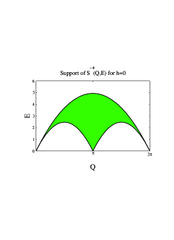
Figure 3.2: The shaded region show where $S^{-+}(Q,E)$ is nonzero for $h=0$. The top boundary corresponds to excitations with two spinons that have identical momentum; on the bottom boundary one of the spinons has fixed momentum $\pm\pi$. $E$ is given in units of $({\scriptstyle\frac{2\pi}{N}})^{2}\frac{v_{s}}{\pi}$.

The main steps of the computation involving the matrix elements $M_{\nu}^{+}$, i.e. the weight of the DSF at a point $(Q,E)$ on the plot, are the following: since $S^{+}_{i}\left|{\rm GS}\right.\rangle$ only contains states with two fully polarized spinons, it must be built out of YHWS. These wavefunctions are functionally identical to eigenfunctions of the Calogero-Sutherland model at coupling $\lambda=2$ of particles moving on a ring. Since both wavefunctions are of a polynomial form with degree $<N$ the computation involving a sum over sites is identical to taking an integral over the ring in the continuum model: $\int_{0}^{N}dn\,e^{ikn}=\sum_{n=0}^{N-1}e^{ikn}$ if $k\in\{-(N-1),\ldots,N-1\}$. The action of $S^{+}_{i}$ in the spin chain is translated into a particle destruction operator $\Psi(x,t)$ ($S^{+}_{i}$ removes a down spin). So the $S^{-+}(Q,E)$ DSF reduces to the Greens function $\langle\left.{\rm GS}\right|\Psi^{\dagger}(x,t)\Psi(0,0)\left|{\rm GS}\right.\rangle$ in the Calogero-Sutherland model. It can be computed in the thermodynamic limit, in which case it can be mapped unto a Gaussian hermitian matrix model correlator. The result is:

$$S^{-+}(Q,E)=\frac{1}{16\pi}\left(\frac{(v_{1}-v_{2})^{2}}{(v_{s}^{2}-v_{1}^{2})(v_{s}^{2}-v_{2}^{2})}\right)^{\frac{1}{2}},$$ (3.10)

with $Q=-\frac{\pi}{2v_{s}}(v_{1}+v_{2})$ and $E=\overline{\epsilon}(v_{1})+\overline{\epsilon}(v_{2})$. The DSF matrix element is parametrized by $v_{1},v_{2}$, which are quickly identified with the velocities of the two spinons in the excited state. The $\langle\Psi^{\dagger}\Psi\rangle$ Greens function has been obtained recently at finite $N$ as well: both the groundstate, the YHWS $|\nu\rangle$ it connects with, and the action of $S^{+}_{i}$ are expressible as symmetric Jack-polynomials, and the matrix element is essentially the Clebsch-Gordan coefficient of the three [Ha94].

For $h\neq 0$ the three different structure functions $S^{-+}(Q,E)$, $S^{zz}(Q,E)$ and $S^{+-}(Q,E)$ will not be equal, since $\left|{\rm GS}\right.\rangle$ is no longer a singlet. In fact it has $S^{z}=S^{tot}=\frac{N_{sp}}{2}\equiv S_{0}$, where $N_{sp}=N_{sp}(h)$ is given by (3.6). This difference between the three correlation function is also expressed in two additional global $SU(2)$ selection rules [M81], which rule out certain matrix elements based on the total spin $S^{tot}$ and $S^{z}$ of the final state $\mu$ inside the Yangian multiplet $\Gamma$.

In the first place there is the Wigner-Eckart theorem for vector operators such as $S^{a}_{i}$, which tells us that in order for $\langle\left.\Gamma,\mu\right|S^{a}_{i}\left|{\rm GS}\right.\rangle$ to be nonzero the total spin $S$ of $\left|\Gamma,\mu\right.\rangle$ must satisfy $S_{0}-1\leq S\leq S_{0}+1$. Secondly, for any state in a multiplet with $N_{sp}$ spinons, we have $\frac{N_{sp}}{2}\geq S\geq S^{z}$—where equality only holds for the YHWS, which has all its spinons up. Now put this together with the fact that $S^{+}_{i}$ raises $S^{z}$ by +1, $S^{-}_{i}$ lowers it by 1, and $S^{z}_{i}$ leaves it the same. Classifying states according to their $S^{z}$ and $S^{tot}$ as types $(i)$ - $(vi)$, following Müller et al. [M81] we find the following contributions:

$S^{+}_{i}\left|{\rm GS}\right.\rangle$

contains states with $S=S_{0}+1$ and $\Delta N_{sp}=+2$ (type $(iii)$ ).

$S^{z}_{i}\left|{\rm GS}\right.\rangle$

contains states with $S=S_{0}+1$ and $\Delta N_{sp}=+2$ (type $(i)$ ) or $S=S_{0}$ and $\Delta N_{sp}=+2,0$ (type $(ii)^{a,b}$ ).

$S^{-}_{i}\left|{\rm GS}\right.\rangle$

contains states with $S=S_{0}+1$ and $\Delta N_{sp}=+2$ (type $(iv)$ ) or $S=S_{0}$ and $\Delta N_{sp}=+2,0$ (type $(v)^{a,b}$ ), or $S=S_{0}-1$ and $\Delta N_{sp}=+2,0,-2$ (type $(vi)^{a,b,c}$ ).

Since we have an additional quantum number to label states: $N_{sp}$, we added Latin superscripts $a,b,c$ to the Roman numerals. All 10 contributions are summarized in table (3.1).

Table 3.1: List of matrix elements contributing to the DSF. The correlation functions in the last column refer to those in the Calogero-Sutherland model as they appear in eqs. (3.10, 3.16, 3.17, 3.23, 3.29, 3.30). The entries marked with a $({\dagger})$ do not survive in the thermodynamic limit. For the example occupation sequences we act on the specific groundstate: $000\rule[-2.5pt]{1.29167pt}{11.00008pt}101010101\rule[-2.5pt]{1.29167pt}{11.00008pt}000$, with the symbols   delimiting the center region. In the column under “Excitation” ${\cal S}$ denotes a spinon and ${\cal M}$ denotes a magnon.

We will now investigate all three structure functions individually following these selection rules.

3.3.1 ${\bf S^{-+}(Q,E)}$

Type $(iii)$: $\Delta N_{sp}=+2$, $\Delta S=+1$.

For the occupation sequence of the groundstate in a given magnetic field (e.g. 
000010101010000) let us label the zeroes in the leftmost orbital as the left spinon condensate and the ones in the rightmost orbital as the right spinon condensate. From table 3.1 we learn that action of $S^{+}_{i}$ on the groundstate only produces states with two more spinons, i.e. one less 1. This 1 has to come out of the center $\cdots 10101\cdots$ region. We can’t take more than a single 1 out of the center region—and place it into the left or right spinon condensate—since this would imply a violation of Rule 1 applied to the center region. Taking out a 1 in the center region is equivalent to inserting 2 spinons there. A typical nonzero matrix element would be $\langle\left.0001001001000,\mu\right|S^{+}_{i}\left|0001010101000\right.\rangle$, with the two spinons residing in orbital two and three.

All this means is that we get a simple two spinon spectrum, as in the zero magnetic field case. The only difference is that now the momenta of the spinons can only vary from $-k_{0}$ to $k_{0}$, where $k_{0}=\frac{\pi}{4N}(N-N_{sp})$ decreases with increasing magnetic field as $N_{sp}=N_{sp}(h)$ according to eq. (3.6). The support of $S^{-+}(Q,E)$ is essentially a squeezed version of Fig. 3.2.

As for the weight associated with 2-spinon excitations: the calculation for the zero magnetic field case (3.10) carries over without problems. The reason for this is twofold. In the first place, the nonzero magnetic field groundstate wavefunction (3.5) is of the same Jastrow-form as the zero field one, with just an extra phase factor $\prod_{i}z_{n_{i}}^{\frac{N}{2}-M}$ appended. When we take the matrix element, the phase factors from ket and bra part cancel each other. Secondly, the excited states are again of the YHWS type $(S=\frac{N_{sp}}{2})$ and have to be polynomials. The mapping onto a Calogero-Sutherland model matrix element remains therefore legitimate.

The contribution of just two-spinon YHWS excitations was to be expected since we can expand any fully polarized localized spinon wavefunction with $N_{sp}$ spinons acted upon with $S^{+}_{i}$ in terms of a set containing $N_{sp}+2$ spinons:

$$(S^{+}_{i}\Psi_{\alpha_{i}})(n_{1},\ldots,n_{M-1})=$$ (3.11)

$$\sum_{p\in V}\prod_{r\in V}\frac{(z_{r}-z_{i})}{(z_{r}-z_{p})}\Psi(n_{1},\ldots,n_{M-1}|\alpha_{1},\ldots,\alpha_{N_{sp}},i,p).$$

Here $V$ is a set of $M$ random sites on the circle excluding the spinon sites $\{\alpha_{i}\}$ (see Appendix B). Eq. (3.9) is a special case of this expansion with $V$ equal to the sites that are an even number of steps removed from the site on which the local spin operator acts. We could also have realized that the number of spinons can’t go up by more than 2 when we consider that $S^{+}$ and $J^{+}_{1}$ annihilate $S^{+}_{i}\left|{\rm GS}\right.\rangle$, indicating that the latter must consist of purely YHWS with $S^{z}=S_{0}+1$!

3.3.2 ${\bf S^{zz}(Q,E)}$

For the DSF $S^{zz}(Q,E)$ we find similar simple excitations that contribute, although at present not all resulting matrix elements can be computed. From the combined selection rules we find three types of excitations: $(i)$, $(ii)^{a}$ and $(ii)^{b}$, in table 3.1. They all have in common that $\Delta N_{sp}=0$ or +2. This isn’t surprising: let us consider the state $J^{+}_{1}\left(S^{z}_{i}\left|{\rm GS}\right.\rangle\right)$. This state is annihilated by $J^{+}_{1}$ and $S^{+}$, so it must be YHWS (see Appendix C). Therefore, since the first action of $J^{+}_{1}$ doesn’t change the number of spinons, $S^{z}_{i}\left|{\rm GS}\right.\rangle$ must be a mixture of states that contain not more than $2S_{0}+2$ spinons, where $2S_{0}$ is the number of spinons in the groundstate.

We will now discuss the individual types and where possible compute the values of the matrix elements.

Type $(i)$: $\Delta N_{sp}=+2$, $\Delta S=+1$.

Having identical selection rules, these states sit in the exact same Yangian- and spin multiplets as the type $(iii)$ states, and therefore they also contain two additional spinons. However their $S^{z}=S^{tot}-1$, so they are no longer YHWS like the type $(iii)$ states. Nevertheless they are related by a simple application of $S^{-}$:

$$|{\scriptstyle\Gamma,\Delta N_{sp}=+2},\!\begin{array}[]{c}{\scriptscriptstyle S^{tot}=S_{0}+1}\\ {\scriptscriptstyle S^{z}=S_{0}}\end{array}\rangle={\scriptstyle\frac{1}{\sqrt{2(S_{0}+1)}}}S^{-}\left|\Gamma\right.\rangle,$$ (3.12)

where $\left|\Gamma\right.\rangle$ denotes the YHWS of the multiplet with occupation sequence $\Gamma$ of type $(iii)$. This allows us to reduce a type $(i)$ matrix element to one that is a multiple of a type $(iii)$ given in eq. (3.10):

$$\left|\langle{\scriptstyle\Gamma,\Delta N_{sp}=+2},\!\begin{array}[]{c}{\scriptscriptstyle S^{tot}=S_{0}+1}\\ {\scriptscriptstyle S^{z}=S_{0}}\end{array}|S^{z}_{i}\left|{\rm GS}\right.\rangle\right|^{2} = {\scriptstyle\frac{1}{2(S_{0}+1)}}\left|\langle\left.\Gamma\right|[S^{+},S^{z}_{i}]\left|{\rm GS}\right.\rangle\right|^{2}$$ (3.15)

$$= {\scriptstyle\frac{1}{2(S_{0}+1)}}\left|\langle\left.\Gamma\right|S^{+}_{i}\left|{\rm GS}\right.\rangle\right|^{2},$$ (3.16)

where we used that $S^{+}$ annihilates the groundstate.

Type $(ii)^{a}$: $\Delta N_{sp}=+2$, $\Delta S=0$.

This type of state is a member of the same kind of Yangian multiplet as type $(iii)$ and $(i)$—i.e. with two extra spinons—but it sits in a spin multiplet that does not contain the YHWS.

Figure 3.3: Graphical illustration of the spin multiplets accessed in $S^{z}_{i}$-excitations of types $(i)$ and $(ii)^{a}$.

States of this kind are supplied by the Algebraic Bethe Ansatz, eq. (1.26): $T^{-}(\lambda_{0})|\Gamma\rangle$. $\lambda_{0}$ is given by eq. (1.27) for $n=1$: $\frac{P(\lambda_{0}+1)}{P(\lambda_{0})}=1$, where $P(u)$ is the Drinfel’d polynomial of occupation sequence $\Gamma$. This equation has a number of trivial solutions, when $\lambda_{0}$ corresponds to two adjacent Drinfel’d roots. These trivial solutions are to be discarded (they correspond to an orbital with more than one spinon in it; these spinons can only be in a symmetric state, and there is a reduction in the naively expected number $2(S_{0}+1)-1$ of $S=S_{0}$ states). The problem is, how to commute the $T^{-}(\lambda_{0})$ through $S^{z}_{i}$ in the matrix element $\langle{\rm GS}|S^{z}_{i}T^{-}(\lambda_{0})|\Gamma\rangle$.

Type $(ii)^{b}$: $\Delta N_{sp}=0$, $\Delta S=0$.

Since this type of state has $\Delta N_{sp}=0$ the number of ones in its occupation sequence must be identical to that in the groundstate. As with the previous three types we can delete just a single 1 from the center, leaving behind two spinons pointing up. This 1 then must go into either the left or the right spinon condensate. Therefore a typical nonzero matrix element would be: $\langle\left.00100\rule[-2.5pt]{1.29167pt}{11.00008pt}1001001\rule[-2.5pt]{1.29167pt}{11.00008pt}00000\right|S^{z}_{i}\left|00000\rule[-2.5pt]{1.29167pt}{11.00008pt}1010101\rule[-2.5pt]{1.29167pt}{11.00008pt}00000\right.\rangle$ where the   just helps to draw attention to the center region. Rule 1 rules out any additional ones leaving the center region. The additional 1 on the left or right can be interpreted as a magnon with $S^{z}=-1$. The limiting case where the magnon “fuses” with two spinons at a boundary between a condensate and the center region gives us the groundstate.

These states must be YHWS since they have $\frac{N_{sp}}{2}=S=S^{z}$, like $\left|{\rm GS}\right.\rangle$. This fact allows us to calculate the corresponding matrix elements. Since both groundstate and excited state are YHWS, a mapping onto the Calogero-Sutherland model is valid. In this case we need a groundstate density-density correlator $\langle\left.{\rm GS}\right|\rho(x,t)\rho(x^{\prime},t^{\prime})\left|{\rm GS}\right.\rangle$ since $S^{z}_{i}$ measures the presence or absence of a down-spin (i.e. a particle in the CS-model). This calculation has been done by Altshuler et al. [A93], in the thermodynamic limit, by studying the repulsion of energy levels in a random matrix model under a varying perturbation. The energy levels are identified with the positions of the particles and the strength of the perturbation corresponds to imaginary time. Their original expression depends on three parameters (called $\lambda,\lambda_{1}$ and $\lambda_{2}$), the latter two of which are compact, and the first one is unbounded. This is precisely what we expect from our selection rule: 2 spinons restricted to the center region with momenta in the range $-k_{0}\ldots+k_{0}$ and a magnon that can go off all the way to the right or left (i.e. $\pm\infty$ in the thermodynamic limit). In terms of the velocity, $v$, of the magnon—with dispersion relation (1.45)—and spinon velocities $v_{1},v_{2}$ their result is as follows:

$$\left|\langle\left.v,v_{1},v_{2}\right|\rho(Q)\left|{\rm GS}\right.\rangle\right|^{2}\propto$$ (3.17)

$$\frac{(v-v_{s})(v+v_{s})|v_{1}-v_{2}|}{\sqrt{(v_{s}^{2}-v_{1}^{2})(v_{s}^{2}-v_{2}^{2})}(v-v_{1})^{2}(v-v_{2})^{2}}\left[(v-v_{1})+(v-v_{2})\right]^{2}.$$

$E=\overline{\epsilon}(v_{1})+\overline{\epsilon}(v_{2})+\epsilon(v)$ and $Q=\frac{\pi}{v_{s}}(v-\mbox{$\frac{1}{2}$}(v_{1}+v_{2}))$. For completeness we give the relation between the $v$’s and the $\lambda$’s :

$$\lambda = v/v_{s}$$

$$\lambda_{1}\lambda_{2} = \frac{(v_{1}+v_{2})}{2v_{s}}$$

$$(1-\lambda_{1}^{2})(1-\lambda_{2}^{2}) = \mbox{$\left(\frac{v_{1}-v_{2}}{2v_{s}}\right)^{2}$}.$$ (3.18)

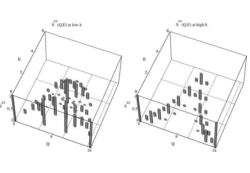
Figure 3.4: $S^{zz}(Q,E)$ for small $h$ $(\sigma=\frac{S_{z}}{N}=.05)$ and large $h$ $(\sigma=.4)$ on $N=14$ sites. $E$ is in units of $({\scriptstyle\frac{2\pi}{N}})^{2}\frac{v_{s}}{\pi}$.

Numerical data for $S^{zz}(Q,E)$ can be found in fig. (3.4) at values of $h$ close to 0 and $h_{c}$. Fig. (3.5) shows the corresponding support of $S^{zz}(Q,E)$ in the $(Q,E)$ plane, as predicted from the selection rule, in the thermodynamic limit. We notice that for finite-size systems some of the features near the lower boundary are absent.

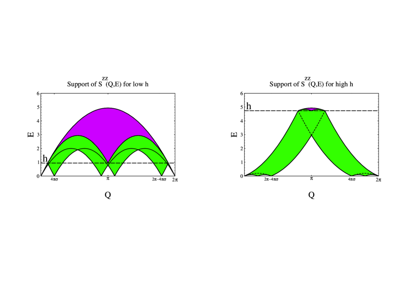
Figure 3.5: The regions where $S^{zz}(Q,E)$ is nonzero for low and high $h$. The area shaded dark contains the contributions from the excitations with $\Delta N_{sp}=+2$ (types ($(i)$ and $(ii)^{a}$). The excitations with $\Delta N_{sp}=0$—type $(ii)^{b}$—can also occupy the lightly shaded area.

3.3.3 ${\bf S^{+-}(Q,E)}$

Finally we discuss the $S^{+-}(Q,E)$ DSF which is governed by the excitations of types $(iv)$ - $(vi)^{c}$ that are present in $S^{-}_{i}\left|{\rm GS}\right.\rangle$.

Type $(iv)$: $\Delta N_{sp}=+2$, $\Delta S=+1$.

This type of state is very similar to types $(iii)$ and $(i)$, as a matter of fact they all reside in identical Yangian- and spin multiplets. Therefore type $(iv)$ states differ from the groundstate only by two extra spinons in the center region. They are related to their YHWS $\left|\Gamma\right.\rangle$ (of type $(iii)$) through:

$$|{\scriptstyle\Gamma,\Delta N_{sp}=+2},\!\begin{array}[]{c}{\scriptscriptstyle S^{tot}=S_{0}+1}\\ {\scriptscriptstyle S^{z}=S_{0}-1}\end{array}\rangle={\scriptstyle\frac{1}{\sqrt{(4S_{0}+2)(2S_{0}+2)}}}(S^{-})^{2}\left|\Gamma\right.\rangle.$$ (3.19)

Analogous to the calculation for type $(i)$ states, a matrix element of type $(iv)$ can now easily be reduced to one involving type $(iii)$:

$$\left|\langle{\scriptstyle\Gamma,\Delta N_{sp}=+2},\!\begin{array}[]{c}{\scriptscriptstyle S^{tot}=S_{0}+1}\\ {\scriptscriptstyle S^{z}=S_{0}-1}\end{array}|S^{z}_{i}\left|{\rm GS}\right.\rangle\right|^{2} = {\scriptstyle\frac{1}{(4S_{0}+2)(2S_{0}+2)}}\left|\langle\left.\Gamma\right|(S^{+})^{2}S^{-}_{i}\left|{\rm GS}\right.\rangle\right|^{2}$$ (3.22)

$$= {\scriptstyle\frac{1}{(2S_{0}+1)(S_{0}+1)}}\left|\langle\left.\Gamma\right|S^{+}_{i}\left|{\rm GS}\right.\rangle\right|^{2}.$$ (3.23)

The last matrix element in this equation has already been computed for the $S^{-+}(Q,E)$ DSF. However the energy of the corresponding excited state here is shifted by $2h$ in comparison, because of the Zeeman term in the Hamiltonian.

Types $(v)^{a}$ and $(vi)^{a}$:$\Delta N_{sp}=+2$, $\Delta S=0,-1$.

States of types $(v)^{a}$ and$(vi)^{a}$ contain a two-spinon excitation as well—like types $(iii)$, $(i)$ and $(iv)$. However, since they don’t reside in the spin multiplet of their YHWS ($\frac{N_{sp}}{2}>S$), the associated matrix elements are unknown. Type $(v)$ can be related to those of type $(ii)^{a}$, though.

$$\left|\langle{\scriptstyle\Gamma,\Delta N_{sp}=0},\!\begin{array}[]{c}{\scriptscriptstyle S^{tot}=S_{0}}\\ {\scriptscriptstyle S^{z}=S_{0}-1}\end{array}|S^{-}_{i}|{\rm GS}\rangle\right|^{2}={\scriptstyle\frac{1}{2S_{0}}}\left|\langle{\scriptstyle\Gamma,\Delta N_{sp}=0},\!\begin{array}[]{c}{\scriptscriptstyle S^{tot}=S_{0}}\\ {\scriptscriptstyle S^{z}=S_{0}}\end{array}|S^{z}_{i}|{\rm GS}\rangle\right|^{2}$$ (3.24)

Type $(vi)^{b}$ is even worse, since it involves the application of two $T^{-}(\lambda)$ operators.

Types $(v)^{b}$: $\Delta N_{sp}=0$, $\Delta S=0$.

Type $(v)^{b}$ states are very similar to those of type $(ii)^{b}$, they only differ in $S^{z}$ by -1. Therefore both contain two excited spinons and a single left- or right moving magnon. They are related to each other by:

$$|{\scriptstyle\Gamma,\Delta N_{sp}=0},\!\begin{array}[]{c}{\scriptscriptstyle S^{tot}=S_{0}}\\ {\scriptscriptstyle S^{z}=S_{0}-1}\end{array}\rangle={\scriptstyle\frac{1}{\sqrt{2S_{0}}}}S^{-}\left|\Gamma\right.\rangle,$$ (3.25)

and $\left|\Gamma\right.\rangle$ is the type $(ii)^{b}$ YHWS of the multiplet with occupation sequence $\Gamma$. We can now trivially relate the matrix elements of type $(ii)^{b}$ and $(v)^{b}$:

$$\left|\langle{\scriptstyle\Gamma,\Delta N_{sp}=0},\!\begin{array}[]{c}{\scriptscriptstyle S^{tot}=S_{0}}\\ {\scriptscriptstyle S^{z}=S_{0}-1}\end{array}|S^{-}_{i}\left|{\rm GS}\right.\rangle\right|^{2} = {\scriptstyle\frac{1}{2S_{0}}}\left|\langle\left.\Gamma\right|[S^{+},S^{-}_{i}]\left|{\rm GS}\right.\rangle\right|^{2}$$ (3.28)

$$= {\scriptstyle\frac{2}{S_{0}}}\left|\langle\left.\Gamma\right|S^{z}_{i}\left|{\rm GS}\right.\rangle\right|^{2}.$$ (3.29)

The last matrix element is listed in eq. (3.17).

Type $(vi)^{b}$: $\Delta N_{sp}=0$, $\Delta S=-1$.

These states reside in the same Yangian multiplets as the previous type however they are not in the spin multiplets of the YHWS: $\frac{N_{sp}}{2}>S=S_{0}-1$. The problem is very similar to that for case $(ii)^{a}$.

Type $(vi)^{c}$: $\Delta N_{sp}=-2$, $\Delta S=-1$.

This last class of states has $\Delta N_{sp}=-2$ and therefore the number of ones in its occupation sequence goes up by one compared to the groundstate. The selection Rule 1 only allows the extra 1 to go into the left or right spinon condensate. As before we are also allowed to take a 1 out of the center region and bring it into the left or right spinon condensate. Notice however that the rule forbids both of the ones to go into the same condensate: one has to be left moving and the other must be right moving. The result is an excited state with two magnons and two spinons. A typical nonzero matrix element would be $\langle\left.0100\rule[-2.5pt]{1.29167pt}{11.00008pt}100101001\rule[-2.5pt]{1.29167pt}{11.00008pt}0001\right|S^{-}_{i}\left|0000\rule[-2.5pt]{1.29167pt}{11.00008pt}101010101\rule[-2.5pt]{1.29167pt}{11.00008pt}0000\right.\rangle$. The   just helps to guide the eye. Also present are YHWS of multiplets from the limiting cases where one of the magnons fuses with the two spinons in the center; this leaves a multiplet with nothing but one magnon; example: $\langle\left.0000\rule[-2.5pt]{1.29167pt}{11.00008pt}101010101\rule[-2.5pt]{1.29167pt}{11.00008pt}0010\right|S^{-}_{i}\left|0000\rule[-2.5pt]{1.29167pt}{11.00008pt}101010101\rule[-2.5pt]{1.29167pt}{11.00008pt}0000\right.\rangle$. This single magnon excitation is familiar from the strong field regime.

Since type $(vi)^{c}$ states are YHWS ($\frac{N_{sp}}{2}=S$), as is the groundstate, we can repeat the calculation of the matrix elements by a mapping onto the Calogero-Sutherland model. Because $S^{-}_{i}$ creates a down spin, it corresponds to a particle creation operator in the CS-model. The relevant correlation function is therefore $\langle\left.{\rm GS}\right|\Psi(x,t)\Psi^{{\dagger}}(x^{\prime},t^{\prime})\left|{\rm GS}\right.\rangle$. As in the $\langle\Psi^{{\dagger}}\Psi\rangle$ case for type $(iii)$ states, a further mapping onto a Gaussian Hermitean matrix model allows one to calculate the Fourier transform of this correlation function [Z93]. The result consists of two parts $G^{(1)}$ and $G^{(2)}$. $G^{(2)}$ is parametrized by four variables, two of which are compact: $|v_{1}|,|v_{2}|<v_{s}$, and two are noncompact:$v<-v_{s},\,v^{\prime}>v_{s}$:

$$\left|\langle\left.v,v^{\prime},v_{1},v_{2}\right|S^{-}(Q)\left|{\rm GS}\right.\rangle\right|^{2}=\hskip 14.45377pt\left\{\frac{(v-v_{1})(v^{\prime}-v_{2})+(v^{\prime}-v_{1})(v-v_{2})}{(v-v^{\prime})}\right\}^{2}$$

$$\hskip 14.45377pt\times\frac{1}{\sqrt{8\pi}}\frac{(v^{2}-v_{s}^{2})(v^{\prime 2}-v_{s}^{2})|v_{1}-v_{2}|}{\sqrt{(v_{s}^{2}-v_{1}^{2})(v_{s}^{2}-v_{2}^{2})}\left[(v-v_{1})(v-v_{2})(v^{\prime}-v_{1})(v^{\prime}-v_{2})\right]^{2}}$$ (3.30)

Energy and momentum in terms of the $v$’s are given by $Q=\frac{\pi}{v_{s}}(v+v^{\prime}-\frac{1}{2}(v_{1}+v_{2}))$ and $E=\frac{\pi}{2v_{s}}(v^{2}+v^{\prime 2}-\frac{1}{2}(v_{1}^{2}+v_{2}^{2})-v_{s}^{2})$. It is obvious that the compact parameters are to be identified with the spinon velocities and the non-compact ones with the magnon velocities. $G^{(1)}$ is parametrized by just one variable $|v|>v_{s}$, which is noncompact

$$\left|\langle\left.v\right|S^{-}(Q)\left|{\rm GS}\right.\rangle\right|^{2}=\frac{1}{2\pi}\frac{v-v_{s}}{v+v_{s}}.$$ (3.31)

This contribution corresponds to the case where one of the magnons has $|v|=v_{s}$, and “fuses” with the two spinons, thus leaving but one magnon.

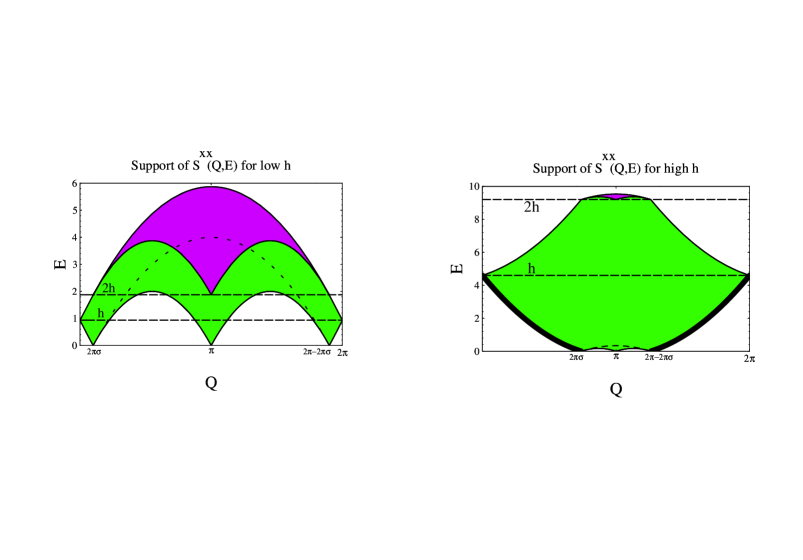
Figure 3.6: Non-zero region of $4S^{xx}(Q,E)=S^{+-}(Q,E)+S^{-+}(Q,E)$ in the $(Q,E)$-plane for low and high $h$. The contributions of $\Delta N_{sp}=+2$ (types $(iv),(v)^{a}$ and $(vi)^{a}$) live in the dark shaded region. These excitations will survive in the limit $h\rightarrow 0$. The $\Delta N_{sp}=0,-2$ can also occupy the area shaded light. For $h\rightarrow h_{c}$ only the 1 magnon contributions survive, as can be seen in Fig. 3.7. These high field magnon excitations are indicated by the thick lines.

Since we now know all possible excitations contributing to $S^{+-}(Q,E)$ we can draw its support in Fig. 3.6 for low and high values of $h$. Fig. 3.7 show numerical data on $S^{+-}(Q,E)$ for those values of $h$. Table 3.1 summarizes the selection rules and available information on matrix elements.

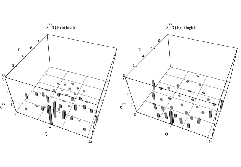
Figure 3.7: $S^{xx}(Q,E)$ for low and high $h$, from numerical diagonalizations on a 10-site chain. $E$ is in units of $({\scriptstyle\frac{2\pi}{N}})^{2}\frac{v_{s}}{\pi}$.

3.4 Comparison to the Bethe Ansatz Model

In 1980 Müller et al. [M81] did a similar calculation of DSFs for the nearest neighbor Heisenberg chain. They identified certain types of states called spin wave continuum states (SWC) as carrying the dominant contribution to the DSFs. These SWC states can be described in a Bethe Ansatz rapidity language by occupation sequences, just like the Yangian multiplets in the ISE model. As it turns out, these SWC states correspond to exactly the same rapidity sequences that are favored by our selection rules in the ISE-model! Although the dispersion relations for the NNE Bethe Ansatz rapidities are different from those in the ISE-model, the authors find the support of the DSFs in the nearest neighbor model to have essentially the same shape as we do in the the inverse exchange case, see fig. 3.8.

However, in the nearest-neighbor Heisenberg chain there are some “anomalous” states, characterized by a change of more than $\pm 2$ spinons, which contribute to a lesser degree to the structure functions and don’t lie within the bounds found by the authors. In the ISE-model these contributions are completely absent and once again we find this model to have a surprisingly clean structure. So in this sense the ISE-model is an ideal spinon gas, whereas in the NNE Heisenberg chain the spinons interact.

Figure 3.8: The $S^{zz}$ structure functions according to Müller et al., Phys. Rev. B 24, 1429 (1981), for $N=10$ in low ($S^{z}_{\rm GS}=2$) and high ($S^{z}_{\rm GS}=4$) magnetic fields. Notice the good match with its ISE counterpart fig. 3.4, except for the low weight NNE states outside the 2-spinon/1-magnon region. The solid lines are boundaries of regions that receive contributions from just 2-spinon excitations. Their dispersion is trigonometric, rather than quadratic, but qualitatively similar.

The characteristic shape of the region in the $Q,E$ plane that carries all (ISE) or most (NNE-model) weight has recently been seen experimentally too [T93]. Tennant et al. scanned along a line in the energy-momentum region with the help of neutrons scattering off ${\rm KCuF}_{3}$ at low (but not too low) temperatures, see fig. 3.9.

Figure 3.9: Neutron scattering data from a quasi one dimensional spin chain ${\rm KCuF}_{3}$ according to Tennant et al.  Phys. Rev. Lett. 70, 4003 (1993). Response is large in regions where the incoming neutrons can excite just two spinons.

The intensity obviously peaks, when traversing the “allowed region”. In the forbidden regions the intensity drops, but not all the way to zero. This might happen because ${\rm KCuF}_{3}$ is better described by a NNE model than by the ISE-model, but the fact that $T\neq 0$ can cause a more smeared distribution too. Finally, there may be non-magnetic scattering centers that contribute to the structure function as well.

Müller et al. also gave general rules, based on comparing Clebsch-Gordon coefficients, determining which matrix elements will survive in the thermodynamic limit. Their conclusion is that the only surviving ones have $S_{\rm Tot}=S^{z}$. This means only excitations $(iii)$ for $S^{-+}(Q,E)$ , $(ii)^{a}$ and $(ii)^{b}$ for $S^{zz}(Q,E)$ and $(vi)^{a}$, $(vi)^{b}$ and $(vi)^{c}$ for $S^{+-}(Q,E)$ remain relevant. (Exceptions are single excitations with $Q=0$, since these correspond to $S^{+}$, $S^{z}$ and $S^{-}$ which give macroscopic contributions, as we can see in the figures). These contributions are trivial to compute.

3.5 Conclusion

We found a remarkably simple selection rule for nonzero matrix elements of local spin operators between eigenstates of the ISE-model, which is reminiscent of the ideal gas single-particle selection rules. One of the consequences of this rule is that the total number of spinons can only change by $0,\pm 2$. Within the occupation sequences this holds locally as well.

In the particular case that one of the states in the matrix element is also the groundstate in a magnetic field (i.e. fully polarized spinons, condensed into the left- and rightmost orbitals in equal amounts), the general selection rule only allows excitations with no more than 2 spinons (the rule applied to the center region) and one left- and one right moving magnon (the rule applied to the condensates on the left and right) . This implies that the structure functions based on the matrix elements involving these states have a finite support in a region dictated by convolving the dispersion relations of these particles (Figs.3.5 and 3.6). These regions have the same shape as those for the nearest neighbor Heisenberg chain. The latter model carries some weight outside these regions as well. Therefore the ISE-model has a much cleaner spinon structure than the NNE-model.

Matrix elements that connect a number of the states in these regions to the groundstate through the local action of a spin operator have been presented. However, information is lacking on those types that involve states not in the spin multiplet of the YHWS. This is particularly bothersome for types $(ii)^{a}$, $(vi)^{a}$ and $(vi)^{b}$ since these will survive in the thermodynamic limit. Their calculation would allow a full reconstruction of the $h\neq 0$ DFS for the ISE-model. A more algebraic treatment involving Yangian operators should provide more insight.

We believe that eventually all dynamical correlation functions of the model will be explicitly found, namely $\langle S(Q,E)\rangle$ at finite magnetic field and temperature. This is a goal that we recommend to future workers on the model. The ability to calculate matrix elements of ${\bf S}_{i}$ between non-YHW states will be a key requirement.

3.6 Appendix.

3.6.1 Appendix A.

We show that localized spinon wavefunctions with $N_{sp}$ spinons all pointing up are necessarily linear combinations of YHWS with exactly $N_{sp}$ spinons. This follows easily from the fact that both $S^{+}$ and $J^{+}_{1}$ annihilate these states. The derivations is very similar to that of Appendix A of chapter 1. If we write $\Psi(n_{1},\ldots,n_{M})=\psi(z_{n_{1}},\ldots,z_{n_{M}})$ where $z_{n}=\exp({\frac{2\pi in}{N}})$ and

$$\psi(w_{1},\ldots,w_{M})=\prod_{i<j}(w_{i}-w_{j})^{2}\prod_{i}w_{i}\prod_{i=1}^{M}\prod_{j=1}^{N_{sp}}(w_{i}-z_{\alpha_{j}}),$$ (3.32)

then

$$(S^{+}\Psi)(n_{1},\ldots,n_{M-1}) = \sum_{j=1}^{N}\Psi(n_{1},\ldots,n_{M-1},j)=\sum_{j=1}^{N}\psi(z_{n_{1}},\ldots,z_{n_{M-1}},e^{\frac{2\pi ij}{N}})$$ (3.33)

$$= \psi(z_{n_{1}},\ldots,z_{n_{M}},0)=0,$$

(where the $\sum_{j}$ was recognized as the zero-mode of a Fourier expansion). And with $w_{jk}=\frac{z_{j}+z_{k}}{z_{j}-z_{k}}$:

$$(J_{1}^{+}\Psi)(n_{1},\ldots,n_{M-1})\sim-\sum_{j=1}^{M}\sum_{i\neq n_{j}}^{N}w_{n_{j},i}\Psi(n_{1},\ldots,n_{M-1},i),$$ (3.34)

where we used the fact that $2S^{z}_{i}=1-2\sum_{j=1}^{M}\delta_{i,n_{j}}$ and that $\Psi$ is a symmetric function which vanishes when two of its arguments coincide. Employing eq. (1.48), we have $J^{+}_{1}\Psi=0$. since $\psi$ has a double zero when two of its arguments coincide and it vanishes at $z=0$.

3.6.2 Appendix B.

In this Appendix we want to prove eq. (3.11). Let us first introduce the following identity which holds for any set of distinct complex numbers $\{\omega_{i}\}$:

$$\prod_{j=1}^{M-1}(Z_{j}-z)=\sum_{k=1}^{M}\prod_{l(\neq k)}^{M}\frac{\omega_{l}-z}{\omega_{l}-\omega_{k}}\prod_{i=1}^{M}(Z_{i}-\omega_{k}).$$ (3.35)

The RHS is just the Lagrange interpolation formula applied to the function in $z$ on the LHS!

Say we want to write $S_{i}^{+}\Psi_{\{\alpha_{i}\}}$ as a linear combination of localized spinon wavefunctions with two more spinons than $\Psi_{\{\alpha_{i}\}}$, and all spinons pointing up. We fix one of the additional two spinons at $i$, the site on which $S^{+}_{i}$ acts, i.e. :

$$(S^{+}_{i}\Psi_{\{\alpha_{i}\}})(n_{1},\ldots,n_{M-1}) \equiv \Psi(n_{1},\ldots,n_{M-1},i|\alpha_{1},\ldots,\alpha_{N_{sp}})$$

$$= \sum_{p(\neq i,\{\alpha_{k}\})}a_{p}\Psi(n_{1},\ldots,n_{M-1}|\alpha_{1},\ldots,\alpha_{N_{sp}},i,p).$$

Using eq. (3.8) we can divide out common factors of $(z_{n_{k}}-z_{n_{l}})$ etc. , and we are left with:

$$z_{i}\prod_{j}(z_{n_{j}}-z_{i})=\sum_{p\neq(i,\{\alpha_{k}\})}a_{p}\prod_{j}(z_{n_{j}}-z_{p}).$$ (3.37)

The result follows when we apply the identity (3.35) to this equation with $z=z_{i}$ and $a_{p}=z_{i}\prod_{k}\frac{z_{k}-z_{i}}{z_{k}-z_{p}}$ where the $z_{k}$ are randomly chosen distinct sites which don’t coincide with the localized spinons.

3.6.3 Appendix C.

We show that $S^{z}_{i}\left|{\rm GS}\right.\rangle$ can only have 0 or 2 more spinons than $\left|{\rm GS}\right.\rangle$ where $\left|{\rm GS}\right.\rangle$ is a YHWS groundstate in a nonzero magnetic field with

$$\langle\left.n_{1},\ldots,n_{M}\right|{\rm GS}\rangle = \Psi_{0}(n_{1},\ldots,n_{M})$$ (3.38)

$$= \prod_{i<j}(z_{n_{i}}-z_{n_{j}})^{2}\prod_{i}z_{n_{i}}^{\frac{N}{2}-M+1}.$$

The proof hinges on the fact that in either of those cases ($\Delta N_{sp}=0$ or $\Delta N_{sp}=+2$) acting on $S^{z}_{i}\left|{\rm GS}\right.\rangle$ twice with $J_{1}^{+}$ will annihilate that state. Potential $\Delta N_{sp}=4,\ldots$ contributions should survive as they are at least 2 levels from the top of their Yangian multiplet. Now

$$(2S^{z}_{i}\Psi_{0})\left({\scriptstyle n_{1},\ldots,n_{M}}\right)=\left(1-2\sum_{j=1}^{M}\delta_{i,n_{j}}\right)\Psi_{0}\left({\scriptstyle n_{1},\ldots,n_{M}}\right),$$ (3.39)

and

$$\left(2J_{1}^{+}S^{z}_{i}\Psi_{0}\right)(n_{1},\ldots,n_{M-1})\sim$$ (3.40)

$$-\sum_{k=1}^{M-1}\sum_{l\neq n_{k}}^{N}w_{n_{k},l}\times\left[\Psi_{0}({\scriptstyle n_{1},\ldots,n_{M-1},l})-2\sum_{j=1}^{M-1}\delta_{i,n_{j}}\Psi_{0}({\scriptstyle n_{1},\ldots,n_{M-1},l})\right]$$

$$-2\sum_{k=1}^{M-1}w_{n_{k},i}\Psi_{0}(n_{1},\ldots,n_{M-1},i)$$

The first two terms vanish when we apply the convolution theorem with $w_{kl}$, as in Appendix 3.6.1; only the last term survives. Notice that the $\{n_{i}\};i=1\ldots,M-1$ cannot be equal to $i$ anymore. This state is trivially annihilated by $S^{+}$ as it vanishes at $z=0$. Furthermore:

$$\left(\left(J_{1}^{+}\right)^{2}S^{z}_{i}\Psi_{0}\right)(n_{1},\ldots,n_{M-2}) = \rule{10.00002pt}{0.0pt}\sum_{p=1}^{M-2}\sum_{q\neq i,n_{p}}^{N}w_{n_{p},q}\sum_{k=1}^{M-2}w_{n_{k},i}\Psi_{0}(n_{1},\ldots,n_{M-2},q,i)$$ (3.41)

$$+\sum_{p=1}^{M-2}\sum_{q\neq i,n_{p}}^{N}w_{n_{p},q}w_{q,i}\Psi_{0}(n_{1},\ldots,n_{M-2},q,i).$$

With the help of the convolution theorem we can set the first term to zero (we can stick in the extra term with $q=i$, which is missing, at no cost since $\Psi_{0}$ vanishes when $q=i$). For the second term we use the identity that lies at the heart of the integrability of the Haldane-Shastry type models: $w_{ij}w_{jk}+w_{jk}w_{ki}+w_{ki}w_{ij}=-1$.

$$\left(\left(J_{1}^{+}\right)^{2}S^{z}_{i}\Psi\right)(n_{1},\ldots,n_{M-2})=$$

$$-\sum_{p=1}^{M-2}\sum_{q\neq i,n_{p}}^{N}(1+w_{i,n_{p}}w_{n_{p},q}+w_{q,i}w_{i,n_{p}})\Psi({\scriptstyle n_{1},\ldots,n_{M-2},q,i}).$$

The first term is zero since $\Psi$ is a polynomial that vanishes at the origin, whereas terms two and three can also be put to zero with the help of the convolution theorem.

Chapter 4 New Types of Off-Diagonal Long Range Order in Quantum Spin-Chains

4.1 Introduction

In this final chapter we attempt to link properties of the ISE-model to some other one and two dimensional correlated systems. We want to show that there exists a new form of Off Diagonal Long Range Order (ODLRO) in 1D spin models; this ODLRO, inspired by electron pair hopping in coupled Hubbard chains or planes, was suggested by Anderson in 1991 [pwaconj]. The corresponding order parameter also has an interesting analogy with the Read-Girvin-MacDonald order parameter in the Fractional Quantum Hall Effect (FQHE) [GM87, Read89]. To be specific, consider the following linear operator $\hat{\Delta}(j)$, acting between the $2^{N-2}$-dimensional $(N-2)$-site spin Hilbert space, and the $2^{N}$ dimensional $N$-site Hilbert space. Acting at site $j$, it consists of slipping in $2$ sites, with two spins in a singlet, between sites $j$ and $j+1$, in the groundstate of a particular model. This operator acquires a non-zero expectation value in the groundstate in the following sense [A66]:

$$\left|\langle 0,N-2|\hat{\Delta}^{\dagger}(j)\hat{\Delta}(0)|0,N-2\rangle\right|^{2} = \left|\sum_{\nu}\langle 0,N-2|\hat{\Delta}^{\dagger}(j)|\nu,N\rangle\langle\nu,N|\hat{\Delta}(0)|0,N-2\rangle\right|$$ (4.1)

$$= \left|\langle 0,N|\hat{\Delta}(0)|0,N-2\rangle\right|^{2}+\ldots$$

$$\rightarrow \;{\rm const}\;\;\;{\rm for}\;N\gg j\gg 1.$$

$|0,N-2\rangle$ is the groundstate on $N-2$ sites, and $\{|\nu,N\rangle\}$ is a complete set of eigenstates of the $N$ site model, where $\nu=0$ labels the groundstate. In the case of translationally invariant models, the first term in the expansion (4.1) guarantees the ODLRO for $\hat{\Delta}(j)$ provided it exceeds $\frac{1}{2}$; in that case the eigenstates have a definite momentum and $\mbox{$\langle 0,N-2|\hat{\Delta}^{\dagger}(j)|\nu,N\rangle$}=e^{i(p_{0}^{N-2}-p_{\nu}^{N})j}\mbox{$\langle 0,N-2|\hat{\Delta}^{\dagger}(0)|\nu,N\rangle$}$. The sum (4.1) is bounded from below by $2\left|\langle 0,N-2|\hat{\Delta}(0)|0,N\rangle\right|^{2}-1$. With the notation:
$a_{\nu}=e^{i(p_{0}^{N-2}-p_{\nu}^{N})j}\cdot$ $\left|\langle\nu,N|\hat{\Delta}(0)|0,N-2\rangle\right|^{2}$, we find this, since $\left|\sum_{\nu}a_{\nu}\right|\geq$ $|a_{0}|-\sum_{\nu>0}|a_{\nu}|$ $=2|a_{0}|-1$ if $|a_{0}|\geq\mbox{$\frac{1}{2}$}$ and $\sum_{\nu}|a_{\nu}|=1$. The last equation is a consequence of the fact that $\hat{\Delta}(0)|0,N-2\rangle$ has norm 1.

We tested for this form of ODLRO for three different 1D models: the short ranged NNE and XY models, and the long ranged ISE-model. In all three cases we find the ODLRO for $\hat{\Delta}$, and (even more remarkably) the constant in eq. (4.1) is almost insensitive to the specific model that we test for: $\sim(0.81)^{2}\approx 0.65$. $\hat{\Delta}(j)$ is mentioned implicitly in [PS], but the context is that of a 1D Hubbard model. We will turn our attention to that in section 4.3.

One might argue that in one dimension only quasi-long range order with algebraic decay of the order parameter correlation function should occur—true LRO being ruled out by the Mermin-Wagner theorem. The way out is that true LRO is allowed if the order parameter either commutes with the Hamiltonian, or if it breaks a discrete symmetry. The latter is the case here, we will find that the singlet insertion breaks the $Z_{2}$ symmetry of shifting by one lattice site.

In the next section we will discuss numerical results and analytical calculations, indicating the presence of the new ODLRO. In section 4.2.2, we will elucidate the analogy between the singlet insertion operator $\hat{\Delta}$ and the Read order parameter in the $\nu=\mbox{$\frac{1}{2}$}$ FQHE. Finally, section 4.3 will illustrate why the LRO for a singlet insertion may have important repercussions for superconducting correlations.

4.2 Evidence of Singlet Insertion ODLRO.

4.2.1 Spin- and Spinon-Singlet Insertion in the ISE-model

Figure 4.1: Overlap between the $(N-2)$-site groundstate with a singlet appended, with the $N$-site groundstate, as a function of N, for three spin models.

In fig. (4.1) we have plotted numerical results for this singlet insertion $\left|\langle 0,N|\hat{\Delta}(j)|0,N-2\rangle\right|$, for the groundstate of the three models mentioned earlier, with Hamiltonian:

$$H=\sum_{i\neq j}J(i-j)\left\{\mbox{$\frac{1}{2}$}(S_{i}^{+}S_{j}^{-}+S_{i}^{-}S_{j}^{+})+\Delta(S_{i}^{z}S_{j}^{z})\right\}.$$ (4.2)

For the XY and NNE models $J(n)=\delta_{n,1}+\delta_{n,-1}$ and $\Delta=0,\,\Delta=1$ respectively. For the ISE-model $J(n)=\frac{1}{(\frac{N}{\pi}\sin(\frac{n\pi}{N}))^{2}}$, $\Delta=1$.

$\hat{\Delta}^{\dagger}(j)\hat{\Delta}(0)$ can be rewritten as

$$\hat{\Delta}^{\dagger}(j)\hat{\Delta}(0)=P_{1,2}^{S}(P_{12\cdots j})^{2}$$ (4.3)

where $P_{12}^{S}$ is the projector for the spins on sites 1,2 onto a singlet: $\frac{1}{4}-{\bf S}_{1}\cdot{\bf S}_{2}$, and $P_{12\cdots j}$ is the operator that cyclically permutes spins on sites $1\cdots j$. With the help of eq. (4.3) we have verified that $\left|\langle 0,N|\hat{\Delta}(0)|0,N-2\rangle\right|^{2}$ is indeed the dominant contribution to $\langle 0|\hat{\Delta}^{\dagger}(j)\hat{\Delta}(0)|0\rangle$ for $N\rightarrow\infty$.

These overlaps are shown as functions of $N$ in fig. 4.1 together with fits to the results of the form $0.817+0.778N^{-2}$ for the ISE model, $0.820+.740N^{-2}$ for the NNE Heisenberg model, and $0.808+0.819N^{-2}$ for the XY model. The results strongly suggest that all overlaps remain finite in the limit where the system size goes to infinity. Note that since the phases of the $N$ and $N-2$ site wavefunctions may be chosen independently the phase of the overlaps is meaningless and further, since the groundstate momenta of the $N$ and $N-2$ site groundstate wavefunctions differ by $\pi$, the overlap is multiplied by minus one if the location of the singlet pair is shifted by one site. We have chosen the overlap real and positive for convenience. As a consequence of this alternation and the finiteness of the overlap, the singlet insertion-singlet deletion correlation function has fixed magnitude and a sign determined by the number of sites between the insertion and the deletion modulo 2 in the limit of infinite separation of the insertion and deletion; the models therefore have a hidden ODLRO which breaks a $Z_{2}$ symmetry. As fig. (4.1) shows, the overlaps for the $N$-site groundstate with the $N-2$ site groundstate with a nearest neighbor singlet insertion in the ISE and Heisenberg models are not only finite in the $N\rightarrow\infty$ limit, but also surprisingly close to each other, despite the fact that the range of the interaction in both models is quite different.

We now present an analytical calculation in the ISE model that gives some understanding of origin of the finite overlap. The unnormalized groundstate wavefunction on $N$ sites of the ISE model in a basis labeled by the positions of the down-spins $\{n_{1},\ldots,n_{M}\}$, $M=\frac{N}{2}$ is given by eq. (1.5):

$$\Psi^{(0)}_{N}\left(n_{1},\ldots,n_{\frac{N}{2}}\right)=\prod_{i=1}^{\frac{N}{2}}(-)^{n_{i}}\prod_{i<j}^{\frac{N}{2}}\sin^{2}\left(\frac{n_{i}-n_{j}}{N}\pi\right)$$ (4.4)

In a basis of local spins $\{|\sigma_{1}\cdots\sigma_{M}\rangle\}$, $\sigma_{i}=\pm\frac{1}{2}$ this reduces to [H91]:

$$\Psi^{(0)}_{M}\{\sigma_{1}\cdots\sigma_{M}\}=\prod_{i<j}^{M}(z_{i}-z_{j})^{\delta_{\sigma_{i},\sigma_{j}}}e^{\frac{\pi i}{2}\rm{sgn}(\sigma_{i}-\sigma_{j})}.$$ (4.5)

For the $N$ site ISE groundstate $M=N$ and $\{z_{i}\}\equiv C_{N}=\{e^{\frac{2\pi in}{N}}\}_{n=1}^{N}$, while for the $N-2$ site groundstate $M=N-2$ and $\{z_{i}\}\equiv C_{N-2}=\{e^{\frac{2\pi in}{N-2}}\}_{n=1}^{N-2}$. To compute the ISE overlap we add $\sigma_{N-1},\;\sigma_{N}$, sitting in a singlet, to the $N-2$ site groundstate. This overlap is not calculable since the $z_{i}$’s from both sets are not commensurate with each other. However, if we slightly deform the set $C_{N-2}$ to be $\{e^{\frac{2\pi in}{N}}\}_{n=1}^{N-2}$ and leave $\sigma_{N-1},\sigma_{N}$ in a singlet then we obtain a new state $\Psi^{(2)}_{N}$, that can be recognized as a localized 2-spinon state [H91, TH94], eq. (3.8), as in fig. (4.2).

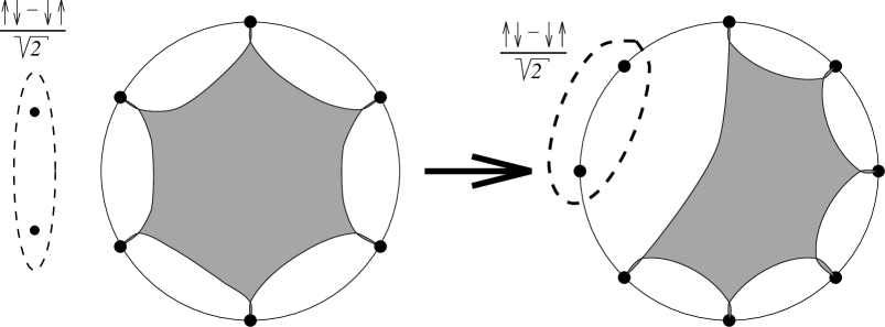
Figure 4.2: Graphical illustration of the deformation of the singlet insertion to a spinon singlet insertion. The gray area is the groundstate wavefunction, or an adiabatic deformation thereof.

This is an uncontrolled approximation whose justification lies in the agreement with our numerical results. This state is an admixture of eigenstates that contain only 0 or 2 “real” spinons. Here the localized spinons sit at sites $N-1$ and $N$ in a singlet. In general we could have put them at sites $\alpha,\beta$ by deforming $C_{N-2}$ into $\{e^{\frac{2\pi in}{N}}|i=1,\ldots,N\}/\{e^{\frac{2\pi i\alpha}{N}},e^{\frac{2\pi i\beta}{N}}\}$.

In the basis of states with $M$ overturned spins with respect to the ferromagnetic state labeled by their positions along the chain: $n_{1},\ldots,n_{M}$, $\Psi^{(0)}_{N}$ and $\Psi^{(2)}_{N}$ are given by :

$$\Psi^{(2)}_{N}\left(n_{1},\ldots,n_{\frac{N}{2}-1}\right)=\prod_{i=1}^{\frac{N}{2}-1}(-)^{n_{i}}\prod_{i<j}\sin^{2}\left({\scriptstyle\frac{n_{i}-n_{j}}{N}\pi}\right)\times\prod_{i=1}^{\frac{N}{2}-1}\sin\left({\scriptstyle\frac{n_{i}-\alpha}{N}\pi}\right)\sin\left({\scriptstyle\frac{n_{i}-\beta}{N}\pi}\right).$$ (4.6)

The overlap between $\Psi^{(0)}_{N}$ and $\Psi^{(2)}_{N}$ for arbitrary separation $\alpha-\beta$ between the spinons is calculated in Appendix A. We find that the normalized overlap is given by:

$$\frac{2}{N}\frac{\sin\left(\pi\frac{\alpha-\beta}{2}\right)}{\sin(\pi\frac{\alpha-\beta}{N})}\sqrt{\frac{\pi(\alpha-\beta)}{{\rm Si}(\pi(\alpha-\beta))}},$$ (4.7)

where ${\rm Si}(x)$ is the Sine integral function. Thus for a nearest neighbor the overlap is $\frac{2}{\pi}\sqrt{\frac{\pi}{{\rm Si}(\pi)}}\simeq 0.82917$, which is within 1.5% of the Heisenberg and ISE groundstate singlet insertion overlaps.

4.2.2 Relation to the FQHE.

We noticed that the action of the generalized singlet insertion operation at sites $\alpha,\beta$, on the ISE-model groundstate was essentially the following: it creates two “holes” at those sites—where the down spins can’t reside—by way of multiplying the wavefunction by a factor $\prod_{i}(z_{n_{i}}-z_{\alpha})(z_{n_{i}}-z_{\beta})$. Then it inserts a down spinon at site $\alpha$, which, in the down spin - particle analogy is just a (hard-core) boson. This all looks very similar to what we know about the bosonic $\nu=\mbox{$\frac{1}{2}$}$ Fractional Quantum Hall Effect. In this theory, particles are constrained to a 2D plane in a very high magnetic field, such that the cyclotron frequency dominates over the interactions between the particles. In that case the Hilbert space is effectively just the set of lowest Landau level wavefunctions, of (kinetic) energy $\mbox{$\frac{1}{2}$}\hbar\omega_{c}=\frac{\hbar eB}{2m}$, which are degenerate. When we turn on interactions, some dramatic things happen: when the filling fraction $\nu=\frac{N}{g}$ is close to a rational number of the from $\frac{1}{m}$, the system develops a gap, and becomes an incompressible fluid with approximate groundstate wavefunction [Laugh]:

$$\Psi(z_{1},\ldots,z_{M})=\prod_{i<j}(z_{i}-z_{j})^{m}e^{-\frac{|z_{i}|^{2}}{4l^{2}}},$$ (4.8)

where $l^{2}=\left|\frac{\hbar}{eB}\right|$ and $z_{i}=x_{i}+iy_{i}$ is the complex co-ordinate of particle $i$. Obviously, for $m$ even the particles must be bosons, and fermions otherwise. Wavefunction (4.8) is valid for particles confined to a circular droplet.

Elementary excitations of this wavefunction are so-called quasiholes and quasiparticles. We will concentrate on the quasiholes. To create one at co-ordinate $z$, we have to introduce an extra zero in the groundstate wavefunction at that point:

$$\Psi(z_{1},\ldots,z_{N}|z)=\prod_{i=1}^{N}(z-z_{i})\,\Psi_{0}(z_{1},\ldots,z_{N}).$$ (4.9)

This is mathematically identical to the up-spinon insertion in the ISE spin wavefunction. A quasihole is a vortex in the quantum hall fluid, that allows one extra flux quantum to pierce the fluid.

The entry into a Quantum Hall phase—with gap—can be signalled by the non-zero expectation value of an order parameter. The Quantum Hall order parameter is not of simple the Bose-condensation type $\psi^{\dagger}({\bf r})$, or Cooper pair type $\psi_{k\uparrow}\psi_{-k\downarrow}$. A first version was suggested by Girvin and MacDonald [GM87]. Soon afterwards, Read introduced his version [Read89]:

$$\hat{O}_{m}(z)=\exp\left(m\int d^{2}z^{\prime}\,\ln(z-z^{\prime})\rho(z^{\prime})\right)\psi^{\dagger}(z),$$ (4.10)

whose effect is to introduce a neutral complex of $m$ quasiholes, and a particle, at co-ordinate $z$. This operator has true long range order in a $\nu=\frac{1}{m}$ Quantum Hall state. Thus, in the limit where the number of sites in the ISE-model becomes large, the spinon-insertion expectation value is essentially the Read order-parameter in the bosonic $m=2$, $\nu=\mbox{$\frac{1}{2}$}$ FQHE, acting at the edge of the circular droplet.

The analogy can be extended further. When the spinon sites are dragged apart, such that $1\ll|\alpha-\beta|\ll N$, we are essentially measuring the spinon propagator. Recall that the localized two spinon wavefunction is a linear combination of eigenstates with two real spinons or none (the groundstate). When we overlap with the latter, we measure the amplitude for one of the spinons to propagate to the other and annihilate (provided that they are in a singlet configuration, since ${\bf S}^{2}$ is conserved). The decay of this propagator $\langle 0,N|(0,\alpha);N-2\rangle$ (where the ket designates the two spinon state) can be derived from eq. (4.7). It is proportional to $\alpha^{-\mbox{$\frac{1}{2}$}}$; $1\ll\alpha\ll N$. We can do the same thing for the singlet insertion, by not inserting the spins in the singlet next to each other, but a distance $\alpha$ apart. This correlator is plotted in fig. (4.3), and shows the same decay $\propto\alpha^{-\mbox{$\frac{1}{2}$}}$.

Figure 4.3: The overlaps between the $N$ site groundstate and the $N-2$ site groundstate with two spins in a singlet inserted at sites 1 and $\frac{N}{2}$. XY model results are from exact numerical results, whereas the ISE-model data for $N>18$ is from Monte Carlo simulations.

We have evidence for the same exponent in the NNE model.

For the $\nu=\mbox{$\frac{1}{2}$}$ FQHE, the corresponding quasihole propagator decays exponentially in the bulk of the material (because of the gap). Low energy excitations can propagate along the edge of the fluid, which is contained by a confining potential. Such modes are called edge states. Quasiholes at the edge have a propagator that decays algebraically, and with Kač-Moody algebra techniques, Wen [Wen] showed that its exponent is $\frac{1}{2}$ as well. As a remarkable aside: the exclusion statistics of the spinons [H91b], which is $\frac{\pi}{2}$ (bosons: 0, fermions $\pi$), is the same as the exchange statistics of the quasiholes in the $\nu=\mbox{$\frac{1}{2}$}$ effect [Arovas].

4.2.3 ODLRO in the XY-model.

In an effort to better understand our results for the Heisenberg and ISE models, we examined the overlap for the same insertion operator acting on the $N-2$ site XY model groundstate with the $N$ site XY model groundstate. The strikingly similar result, here extended to a larger system size than was possible for the Heisenberg and ISE models, is shown in fig. 4.1. Since the XY model can be mapped onto spinless fermions, the “order parameter” can be recast in that language and a more detailed study made. In that language the non-zero overlap is between the groundstate for $N/2$ spinless fermions, with either periodic of antiperiodic boundary conditions, on $N$ sites (with positive hopping integral so that their momentum in the groundstate are centered around $\pi$) and the state obtained by adding two sites and one fermion (in a superposition of being on the two added sites with a relative minus sign for the two different sites) to the groundstate for the $\frac{N}{2}-1$ spinless fermions on $N-2$ sites with the opposite boundary conditions from the $N$ site case. The change of boundary conditions is a non-local operation in the fermion language, however in the spin language it arises from a local operation, i.e. the insertion of two additional spins in a singlet configuration.

Since the wavefunctions for the two fermion states are just Slater determinants, we can bound the singlet insertion matrix element rigorously from below. The technical details can be found in Appendix B. It is found there that $|\langle 0,N|\hat{\Delta}(j)|0,N-2\rangle|$ $>e^{-\frac{5}{2}}$ for $N\rightarrow\infty$.

It is somewhat remarkable that the ODLRO for the XY-model is the result of three conspiring effects, every one of which by itself would lead to a vanishing matrix element as $N\rightarrow\infty$.

• $|0,N\rangle$ had $\frac{N}{2}$ electrons, all in extended states and $\hat{\Delta}(j)|0,N-2\rangle$ has $\frac{N}{2}-1$ electrons in extended states too, but the last is in a localized two site state, resulting in a decay $\propto\frac{1}{\sqrt{N}}$.

• The extended states in the $N$-particle groundstate have periodicity $N$, whereas the $(N-2)$-particle groundstate has periodicity $N-2$, with a resulting orthogonality type catastrophe in the overlap.

• The particles in the $N$-site groundstate have periodic/antiperiodic boundary conditions, whereas the $(N-2)$-site version has antiperiodic/periodic ones (depending on the parity of $\frac{N}{2})$.

For the XY-model too, we have done numerical calculations, studying the decay of the singlet insertion as a function of the separation of the singlet spins, see fig. (4.3). In this case we find an exponent very close to $\frac{5}{8}$. In the next section we will give arguments for this particular decay exponent from the point of view of the Luttinger liquid picture, which describes the low energy excitations of these spin models [Haldane].

Finally, the XY model and the ISE model both have wavefunctions of the Jastrow product form of the Calogero-Sutherland model [Suth71, Hald88]:

$$\Psi^{(0)}_{N}\left(n_{1},\ldots,n_{\frac{N}{2}}\right)=\prod_{i=1}^{\frac{N}{2}}(-)^{n_{i}}\prod_{i<j}^{\frac{N}{2}}\sin^{p}\left(\frac{n_{i}-n_{j}}{N}\pi\right)$$ (4.12)

For the XY model $p=1$ whereas for the ISE model $p=2$. We have studied numerically the overlap for a number of values of $p$ and find that it remains finite in the limit of large system size and is essentially constant for $1\leq p\leq 2$. We have also examined $0\leq p\leq 1$ and find the overlap to be finite in the large system size limit and monotonically decreasing with $p$ down to a value of $1/2$ at the point $p=0$ where the wavefunction is that of Gutzwiller projected free bosons and the can be computed exactly as $\frac{1}{\sqrt{2}}\sqrt{\frac{N}{N-1}}$. Note that this implies $O(\frac{1}{N}))$ corrections in contrast to the $O(\frac{1}{N^{2}})$ corrections we find for the XY, ISE and Heisenberg models. It is not clear when corrections of size $O(\frac{1}{N})$ first appear.

It may be tempting, based on the similarity of the wavefunctions (4.12) to relate the XY model ODLRO to a $\nu=1$ Read order parameter, acting on the edge. However, the singlet decay exponent $\frac{5}{8}$ is not consistent with the electron propagator exponent in the Quantum Hall situation.

4.3 Singlet Insertion in the 1D Hubbard Model.

In the context of spin models, the singlet insertion operation may seem somewhat esoteric, requiring the Hilbert space to change size. Now if we imagine the sites to be physical electrons, then the singlet insertion procedure corresponds to hopping two electrons in a singlet configuration onto a chain.

We follow the tradition of studying spin models in the guise of the 1D Hubbard model in the limit of one particle/site, and $U\rightarrow\infty$ [HA87], and consider the action of our order parameter in the context of this simplest of interacting 1D itinerant electron models. Its Hamiltonian is given by:

$$H=t\sum_{is}(c_{i\sigma}^{\dagger}c_{i+1\sigma}+{\rm h.c.})+U\sum_{i}n_{i\uparrow}n_{i\downarrow}.$$ (4.13)

The $i$’s are site-labels. The $U>0$ term discourages electrons to occupy the same site. There is an additional non-academic reason to study the effects of singlet insertion in a Hubbard-type model. One of the mechanisms to explain the high transition temperatures in the copper-oxide superconductors is built around the relevance of the hopping of electron singlet pairs between the 2D layers in these materials [pwaconj]. We will attempt to decide on the relevance of this operator in the one-dimensional Hubbard model for $U\rightarrow\infty$, based on the ODLRO of our singlet insertion (see [Strong95] for possible ways to extend this procedure to two dimensions). The inter-chain hopping operator acting at sites $j,j+1$ is given by:

$${\cal O}_{S}(j) = \mbox{$\frac{1}{2}$}(c_{j\uparrow}^{\dagger}c_{j+1\downarrow}^{\dagger}-c_{j\downarrow}^{\dagger}c_{j+1\uparrow}^{\dagger})(d_{j\uparrow}d_{j+1\downarrow}-d_{j\downarrow}d_{j+1\uparrow})+{\rm h.c.}$$ (4.14)

$$\equiv {\cal O}_{1}(j){\cal O}_{2}^{\dagger}(j)+{\rm h.c.},$$

where $c_{j\sigma}^{\dagger}$ are the electron creation operators for chain 1, and the $d$’s act on chain 2. The relevance of this operator in the renormalization group sense for perturbing away form the uncoupled chain case, is determined by its scaling dimension $d_{s}$ in $\langle 0|{\cal O}_{S}^{\dagger}(j){\cal O}_{S}(0)|0\rangle\sim j^{-2d_{s}}$ for $j\rightarrow\infty$. If $d_{s}>2$, singlet pair hopping is irrelevant. $|0\rangle$ is the tensor product groundstate of the two uncoupled Hubbard models. The ${\cal O}_{S}$-${\cal O}_{S}$ correlator then factorizes into an $\langle{\cal O}_{1}^{\dagger}(j){\cal O}_{1}(0)\rangle$ and $\langle{\cal O}_{2}^{\dagger}(j){\cal O}_{2}(0)\rangle$ part. Ogata and Shiba have pointed out an additional simplification for large $U$ [OgataShiba]: the groundstate of (4.13), for $M$ electrons, factorizes into the convolution of a spin and a charge part:

$$\Psi_{0}(n_{1},\ldots,n_{M}|\sigma_{1},\ldots,\sigma_{M})=\Psi_{\rm SF}(n_{1},\ldots,n_{M})\chi(\sigma_{1},\ldots,\sigma_{M}),$$ (4.15)

where $\Psi_{\rm SF}$ is the determinantal groundstate wavefunction of $M$ free spinless fermions, labeled by co-ordinates $\{n_{i}\}$. $\chi(\sigma_{1},\ldots,\sigma_{M})$ is the groundstate of the NNE Heisenberg model (at least for $N=4m+2$, $m$ integer) of $M$ spins, residing on the spinless fermions. Then $\langle 0_{1}|{\cal O}_{1}^{\dagger}(j){\cal O}_{1}(0)|0_{1}\rangle$ reduces further to:

$$\langle\Psi_{\rm SF}|\psi_{j+1}\psi_{j}\psi_{1}^{\dagger}\psi_{0}^{\dagger}(-)^{\sum_{i(<j)}n_{i}}|\Psi_{\rm SF}\rangle\cdot\left|\langle\chi|\hat{\Delta}(j)^{\dagger}\hat{\Delta}(0)|\chi\rangle\right|$$ (4.16)

$\hat{\Delta}$ is the singlet insertion order parameter from the spin models which alternates with $j$, i.e. keeps track of the number of fermions to the left of the insertion site, whence the $(-)^{\sum_{i(<j)}n_{i}}$ factor in the spinless fermion matrix element. $\psi_{i},\psi_{i}^{\dagger}$ are spinless fermion operators. The second factor in eq. (4.16) is constant ($\sim 0.65$ as we saw before).

The matrix element decay eq. (4.16) then follows from the fact that free fermion operators have dimension 1 and the alternating term has dimension $\frac{1}{2}$. We want to derive this a bit more extensively in a bosonized language in the original Hubbard model. We will also include a spin anisotropy term to accommodate the XY model limit later on. In the continuum limit the $c_{js}\rightarrow\psi_{R,s}(ja)+\psi_{L,s}(ja)$, the field operators acting at the left and right Fermi points. $s=\pm\mbox{$\frac{1}{2}$}$ is the spin label, and $a$ the lattice spacing. In one dimension they can be rewritten in terms of boson fields [Haldane, Schulz93]:

$$\psi_{\rule{0.0pt}{2.79996pt}^{R}_{L}s}(j) = \lim_{\alpha\rightarrow 0}\frac{1}{\sqrt{2\pi\alpha}}e^{\pm ik_{F}x-i(\pm\frac{\phi_{\rho}+s\phi_{\sigma}}{\sqrt{2}}-\frac{\theta_{\rho}+s\theta_{\sigma}}{\sqrt{2}})}$$ (4.17)

$$\equiv e^{\pm ik_{F}x-i\Theta_{\rule{0.0pt}{1.99997pt}^{R}_{L}s}(x)}.$$

$\alpha$ is a cut-off scale. The fields $\phi_{\mu}$ and $\partial_{x}\theta_{\mu}$, $\mu=\rho,\sigma$ are canonically conjugate bosonic fields: $[\phi_{\mu}(x),\partial_{x}\theta_{\nu}(x^{\prime})]=i\pi\delta_{\mu\nu}\delta(x-x^{\prime})$. One also writes $\Pi_{\mu}=\pi\partial_{x}\theta_{\mu}$. The fields with label $\sigma$ create/annihilate spin excitations (destroy up- and create down-spin electrons and vice-versa); the $\rho$-fields relate to charged excitations. A peculiarity of the 1D Hubbard model is that these fields propagate independently: spin-charge separation, as is evident from the Hamiltonian in the bosonic language:

$$H = \int dx\,\left\{\frac{\pi v_{c}K_{\rho}}{2}\Pi_{\rho}^{2}+\frac{v_{c}}{2\pi K_{\sigma}}(\partial_{x}\phi_{\rho})^{2}\right\}$$ (4.18)

$$+\int dx\,\left\{\frac{\pi v_{s}K_{\sigma}}{2}\Pi_{\sigma}^{2}+\frac{v_{s}}{2\pi K_{\sigma}}(\partial_{x}\phi_{\sigma})^{2}+\hat{g}\cos(\sqrt{8}\phi_{\sigma})\right\}+\ldots$$

The ellipses refer to other irrelevant terms originating from the non-linear electron dispersion relation and the underlying lattice. $v_{c}$ and $v_{s}$ are the velocities of spin and charge excitations respectively. $K_{\rho}$ and $K_{\sigma}$ are functions of the Hubbard parameters. All correlation function exponents can be expressed in terms of these two. The spin cosine term is irrelevant if $0<U<\infty$ and the anisotropy $\Delta$ satisfies $-1<\Delta\leq 1$. The non-linear term only acts to renormalize $K_{\rho}$ and $K_{\sigma}$: $K_{\rho}(U=0)=1$, $K_{\rho}(U\rightarrow\infty)$$=\mbox{$\frac{1}{2}$}$, and $K_{\sigma}(\Delta,U\rightarrow\infty)$ $=1-\frac{1}{\pi}\arccos(\Delta)$ [Affleck]. So at long wavelengths, we have two uncoupled free linearly dispersing bosons with different velocities. The electronic correlation functions can be deduced from the bosonic ones via (4.17). The latter are easy to compute, since the fixed point Hamiltonian is quadratic. For example [Emery79]:

$$\langle e^{i\alpha\theta_{R\mu}(x,t)}e^{-i\beta\theta_{R\mu}(0,0)}\rangle=\left(\frac{1}{(x-v_{\mu}t)^{\frac{K_{\mu}}{4}+\frac{1}{4K_{\mu}}+\mbox{$\frac{1}{2}$}}}\frac{1}{(x+v_{\mu}t)^{\frac{K_{\mu}}{4}+\frac{1}{4K_{\mu}}-\mbox{$\frac{1}{2}$}}}\right)^{\alpha\beta},$$ (4.19)

Notice that for interacting electrons ($K_{\mu}\neq 1$) a right Fermi point electron operator has an antiholomorphic part too!

In the following we will neglect the phase-factors, since we are just interested in the scaling dimensions. Consider the case where the singlet electrons are inserted, not as nearest neighbors, but at sites $x,x^{\prime}$, and extracted at sites $y,y^{\prime}$: $\langle 0|\psi_{\uparrow}^{\dagger}(x)\psi_{\downarrow}^{\dagger}(x^{\prime})\psi_{\uparrow}(y)\psi_{\downarrow}(y^{\prime})|0\rangle+\ldots$, where $1\ll|x-x^{\prime}|,|y-y^{\prime}|\ll|x-y|$ in units of the lattice spacing $a$. In this limit we can then apply the operator product expansion of fields $\psi^{\dagger}(x)$ and $\psi^{\dagger}(x^{\prime})$ and separately $\psi(y)$ and $\psi(y^{\prime})$. In terms of the bosons:

$$e^{i\theta_{R\uparrow}(xt)}e^{i\theta_{R\downarrow}(x^{\prime}t^{\prime})} \sim \left[e^{\frac{i}{\sqrt{2}}\theta_{R\rho}(xt)}\cdot e^{\frac{i}{\sqrt{2}}\theta_{R\rho}(x^{\prime}t^{\prime})}\right]\left[e^{\frac{i}{\sqrt{2}}\theta_{R\sigma}(xt)}\cdot e^{-\frac{i}{\sqrt{2}}\theta_{R\sigma}(x^{\prime}t^{\prime})}\right]$$ (4.20)

$$\stackrel{{\scriptstyle x^{\prime},t^{\prime}\rightarrow x,t}}{{\sim}} (\Delta x-v_{c}\Delta t)^{p_{\rho}+\frac{1}{4}}(\Delta x+v_{c}\Delta t)^{p_{\rho}-\frac{1}{4}}:e^{i\sqrt{2}\theta_{R\rho}(xt)}:$$

$$\times\frac{1}{(\Delta x-v_{s}\Delta t)^{p_{\sigma}+\frac{1}{4}}(\Delta x+v_{s}\Delta t)^{p_{\sigma}-\frac{1}{4}}}:\mbox{1l}+\ldots:,$$

where $p_{\rho}=\frac{1}{8K_{\rho}}+\frac{K_{\rho}}{8}$ and $p_{\sigma}=\frac{1}{8K_{\sigma}}+\frac{K_{\sigma}}{8}$. We used the generalization of the Glauber formula: $e^{A}e^{B}=:e^{A+B}e^{\langle 0|AB+\frac{A^{2}+B^{2}}{2}|0\rangle}$ for normal ordering with respect to the bosonic vacuum, and $A,B$ commuting with their commutators [Shankar91]. There is a term with identical exponents for $R\rightarrow L$, and less relevant terms, containing mixtures of both. Notice that the equal-time singlet insertion decay exponent of fig. (4.3) can be read off from (4.20): $2p_{\sigma}=\frac{K_{\sigma}}{4}+\frac{1}{4K_{\sigma}}=\mbox{$\frac{1}{2}$}$ for $\Delta=1$ (NNE-model limit) and $\frac{5}{8}$ for $\Delta=0$ (XY-model limit).

The part of the electron singlet operator that yields the spin-singlet correlator is $e^{\frac{i}{\sqrt{2}}\theta_{R\sigma}(x)}$. This operator is semionic, in that commuting two of these through each other results in a phase $e^{\frac{\pi i}{2}}$, for the isotropic Hubbard model. This is compatible with the earlier observation that the singlet insertion is essentially a two-spinon creation operator. [ludwig] suggests a semionic operator in the context of a CFT realization of the low energy part of the ISE-model, bilinears of whose Fourier modes create 2 spinons as well. An identification of the boson-exponential with this CFT operator seems appropriate.

From eq. (4.20) we learn that the electron singlet insertion in bosonized form is $e^{i\sqrt{2}\theta_{R\rho}}$, with dimension $\frac{5}{4}$ and correlator decay $\propto(x-y)^{-\frac{5}{2}}$, as we found before (see also [Haldane, hubb_ll, Frahm]). The expression for ${\cal O}$ contains a charge-prefactor which grows with separation between the singlet spins, since it has a negative scaling dimension. This need not concern us, since this separation is bounded from above by the distance to the singlet extraction, i.e., the OPE is no longer valid when $x^{\prime}\approx y,y^{\prime}$.

The decay exponent $\frac{5}{2}$ is insufficient to make singlet pair hopping between chains relevant. From our spin model singlet insertion, we find the culprit to be the operator $(-)^{\sum_{i(<j)}n_{i}}$, caused by the alternation of the spin order parameter. It has been suggested [Strong95] that this can be remedied if it could be canceled against a similar alternating factor in the second chain.

4.4 Conclusion.

We have shown that the operator that inserts a singlet into a 1D spin chain acquires LRO in the ISE-, XY- and NNE-models. We provided numerical evidence and suggested that its LRO might be expected based on its interpretation as a two spinon insertion, as well as via an analogy to Read’s order parameter in the $\nu=\mbox{$\frac{1}{2}$}$ QHE (for NNE and ISE-models). The fact that the order parameter breaks a $Z_{2}$ symmetry causes the more physical electron singlet hopping operator in coupled 1D Hubbard chains to become irrelevant. Bosonizing the anisotropic Hubbard chain allows us to calculate the decay exponent of the spin singlet insertion operator or, equivalently, the spinon propagator, as a function of the anisotropy.

The fact that this ODLRO is present in three quite different antiferromagnetic isotropic spin-chains, raises the question whether there are models where it doesn’t occur. XY-, ISE- and NNE- models are all gapless and one might imagine that that is a key feature to this particular ODLRO, but for instance the Majumdar-Ghosh model with a gap above its dimerized groundstate possesses the singlet-insertion ODLRO by definition. This is an important issue since the usefulness of the order-parameter depends on its ability to discriminate between different models.

4.5 Appendix

4.5.1 Appendix A: The Two-Spinon Matrix Element

We compute the (normalized) overlap between the $N$-site ISE groundstate $|\Psi^{(0)}\rangle$ and the $N$-site two-spinon wavefunction, localized at sites $\alpha$ and 0, $|\Psi^{(2)}(\alpha)\rangle$. The two-spinon wavefunction is an adiabatic deformation of the $(N-2)$-site groundstate plus a singlet. Because of translational invariance we can fix $\beta$ to be 0. What we need to compute is:

$$\frac{\langle\Psi^{(0)}|\Psi^{(2)}(\alpha)\rangle}{\sqrt{\langle\Psi^{(0)}|\Psi^{(0)}\rangle\langle\Psi^{(2)}(\alpha)|\Psi^{(2)}(\alpha)\rangle}}=\frac{\langle\Psi^{(0)}|\Psi^{(2)}(\alpha)\rangle}{\langle\Psi^{(0)}|\Psi^{(0)}\rangle}\left(\frac{\langle\Psi^{(2)}(\alpha)|\Psi^{(2)}(\alpha)\rangle}{\langle\Psi^{(0)}|\Psi^{(0)}\rangle}\right)^{-\frac{1}{2}}\equiv A\cdot B^{-\mbox{$\frac{1}{2}$}}$$ (4.21)

First we will determine $\langle\Psi^{(0)}|\Psi^{2}(\alpha)\rangle$. Setting $M=\frac{N}{2}-1$:

$$\langle\Psi^{(0)}|\Psi^{(2)}(\alpha)\rangle = {\scriptstyle\left(\frac{N}{2}\right)}!~{}\sum_{n_{1},\ldots,n_{M}}\frac{1}{\sqrt{2}}\Psi^{(2)}(n_{1},\ldots,n_{M}|0,\alpha)\times$$ (4.22)

$$\left\{\Psi^{(0)}(n_{1},\ldots,n_{M},0)-\Psi^{(0)}(n_{1},\ldots,n_{M},\alpha)\right\}^{*}$$

$$= \frac{1}{\sqrt{2}}{\scriptstyle\left(\frac{N}{2}\right)}!~{}\sigma(\alpha)\left(1-(-)^{\alpha}\right).$$

Here

$$\sigma(\alpha) = \sum_{n_{1},\ldots,n_{M}}\left(\prod_{i<j}\sin^{4}\left(\frac{n_{i}-n_{j}}{N}\pi\right)\right)$$ (4.23)

$$\times \prod_{i=1}^{M}\sin^{3}\left(\frac{\pi n_{i}}{N}\right)\prod_{i=1}^{M}\sin\left(\frac{n_{i}-\alpha}{N}\pi\right).$$

In eq. (4.22) we shifted all the $n_{i}$ by $\alpha$ in the second term to bring both terms in the same form.

Since $\Psi^{(0)}$ is a singlet, we know that if the two spinons in $\Psi^{(2)}$ were in the $S_{z}=0$ triplet state the overlap should be zero, i.e. $\langle\Psi^{(0)}|\Psi^{(2)}(\alpha),{\rm triplet}\rangle\propto\sigma(\alpha)\left(1+(-)^{\alpha}\right)=0$ for all $\alpha$. Therefore $\sigma(\alpha)$ vanishes for all even $\alpha$. At the same time we see from eq. (4.22) that $\sigma(\alpha)$ is a polynomial in $\cos\left(\frac{\pi\alpha}{N}\right)$. This is easily checked by expanding the $\sin\left(\frac{n_{i}-\alpha}{N}\pi\right)$ and noting that $\sigma(\alpha)$ is even in $\alpha$. We conclude immediately  [gradryz]:

$$\sigma(\alpha) \propto \prod_{j=1}^{\frac{N}{2}}\left(\cos\left(\frac{\pi\alpha}{N}\right)-\cos\left(\frac{2\pi j}{N}\right)\right)$$ (4.24)

$$\propto \frac{\sin\left(\frac{\pi\alpha}{2}\right)}{\sin\left(\frac{\pi\alpha}{N}\right)}.$$

which holds, even when $\alpha$ is not integer. This gives us the $\alpha$ dependence in $A$. To get the normalization correctly, let us write out $A$ ($\alpha$ odd):

$$A = \frac{1}{\sqrt{2}}\frac{\left(\frac{N}{2}\right)!\cdot 2\cdot\sum_{n_{1},\ldots,n_{M}}\prod_{i<j}\sin^{4}\left(\frac{n_{i}-n_{j}}{N}\pi\right)\prod_{i}\sin^{3}\left(\frac{n_{i}}{N}\pi\right)\sin\left(\frac{n_{i}-\alpha}{N}\pi\right)}{\left(\frac{N}{2}\right)!\cdot\sum_{n_{1},\ldots,n_{M+1}}\prod_{i<j}\sin^{4}\left(\frac{n_{i}-n_{j}}{N}\pi\right)}$$ (4.25)

$$= \frac{2\sum_{n_{1},\ldots,n_{M}}\prod_{i<j}\sin^{4}\left(\frac{n_{i}-n_{j}}{N}\pi\right)\prod_{i}\sin^{3}\left(\frac{n_{i}}{N}\pi\right)\sin\left(\frac{n_{i}-\alpha}{N}\pi\right)}{\sqrt{2}N\sum_{n_{1},\ldots,n_{M}}\prod_{i<j}\sin^{4}\left(\frac{n_{i}-n_{j}}{N}\pi\right)\prod_{i}\sin^{4}\left(\frac{\pi n_{i}}{N}\right)}.$$

In the last step we changed the summation variables $n_{i}\rightarrow n_{i}+n_{M+1};i=1,\ldots,M$ in the denominator and did the trivial $n_{M+1}$ summation. Despite the fact that physically $\alpha$ is actually an integer, we can formally take the limit $\alpha\rightarrow 0$ in the last expression and obtain: $A(\alpha=0)=\frac{\sqrt{2}}{N}$. Therefore:

$$A=\frac{4}{\sqrt{2}N^{2}}\frac{\sin(\frac{\pi\alpha}{2})}{\sin(\frac{\pi\alpha}{N})}$$ (4.26)

Now we turn our attention to the second piece. Only its numerator is $\alpha$ dependent:

$$\langle\Psi^{(2)}(\alpha)|\Psi^{(2)}(\alpha)\rangle=$$ (4.27)

$$\left(\frac{N}{2}-1\right)!~{}\sum_{\{n_{1},\ldots,n_{M}\}}\left(\Psi^{(2)}(n_{1},\ldots,n_{M}|0,\alpha)\right)^{2}$$

$$=2\left(\frac{N}{2}-1\right)!~{}\sum_{n_{1},\ldots,n_{M}}\prod_{i<j}\sin^{4}\left(\frac{n_{i}-n_{j}}{N}\pi\right)\times$$

$$\hskip 10.84006pt\prod_{i=1}^{M}\sin^{2}\left(\frac{\pi n_{i}}{N}\right)\sin^{2}\left(\frac{n_{i}-\alpha}{N}\pi\right).$$

But this sum can be recognized as the $\langle S^{z}(\alpha)S^{z}(0)\rangle$ static correlation function in the ISE model [Hald88], or—after an (exact) conversion of the sums to integrals (see chapter 3)—as the one-particle density matrix in the Calogero-Sutherland model at half filling [Suth71, Hald88]. The result for large $N$ is proportional to $\frac{{\rm Si}(\pi\alpha)}{\pi\alpha}$, where ${\rm Si}(x)$ is the sine-integral function $\int_{0}^{x}dx^{\prime}\,\frac{\sin(x^{\prime})}{x^{\prime}}$. To normalize $B$ properly we write it out:

$$B = \frac{\left(\frac{N}{2}-1\right)!\cdot\sum_{n_{1},\ldots,n_{M}}\prod_{i<j}\sin^{4}\left(\frac{n_{i}-n_{j}}{N}\pi\right)\prod_{i}\sin^{2}\left(\frac{n_{i}}{N}\pi\right)\sin^{2}\left(\frac{n_{i}-\alpha}{N}\pi\right)}{\left(\frac{N}{2}\right)!\cdot\sum_{n_{1},\ldots,n_{M+1}}\prod_{i<j}\sin^{4}\left(\frac{n_{i}-n_{j}}{N}\pi\right)}$$ (4.28)

$$= 2\cdot\frac{\sum_{n_{1},\ldots,n_{M}}\prod_{i<j}\sin^{4}\left(\frac{n_{i}-n_{j}}{N}\pi\right)\prod_{i}\sin^{2}\left(\frac{n_{i}}{N}\pi\right)\sin^{2}\left(\frac{n_{i}-\alpha}{N}\pi\right)}{N^{2}\sum_{n_{1},\ldots,n_{M}}\prod_{i<j}\sin^{4}\left(\frac{n_{i}-n_{j}}{N}\pi\right)\prod_{i}\sin^{4}\left(\frac{\pi n_{i}}{N}\right)}.$$

In the last step we shifted the summation variables, as we did previously for $A$, to simplify the denominator. We now recognize that for $\alpha=0$, $B=2/N^{2}$. As for $A$, the normalization can be obtained from the case $\alpha=0$ and we find:

$$B=\frac{2}{N^{2}}\frac{{\rm Si}(\pi\alpha)}{\pi\alpha},$$ (4.29)

The entire expression for the overlap, with normalization, then becomes:

$$\frac{2}{N}\frac{\sin\left(\frac{\pi\alpha}{2}\right)}{\sin(\frac{\pi\alpha}{N})}\sqrt{\frac{\pi\alpha}{{\rm Si}(\pi\alpha)}}.$$ (4.30)

4.5.2 Appendix B: Lower Bound on the XY ODLRO

We want to show that $\langle 0,N|\hat{\Delta}(j)|0,N-2\rangle$ is finite when $N\rightarrow\infty$. We begin, following Anderson’s treatment of the orthogonality catastrophe [pwaorthog], by writing the overlap as the $\frac{N}{2}\times\frac{N}{2}$ determinant of of the matrix formed from the inner products of the single particle wavefunctions comprising the two states:

$${\rm overlap}=|M_{i,j}|=\left|\langle\Psi_{i}^{(1)}|\Psi^{(2)}_{j}\rangle\right|$$ (4.31)

where, for $\frac{N}{2}$ an odd integer and periodic boundary conditions for the $N$ site case:

$$|\Psi_{k}^{(a)}\rangle=\sum_{n=1}^{N+2(1-a)}\frac{(z_{k,a})^{n}}{\sqrt{N+2(1-a)}}|n\rangle$$ (4.32)

except that

$$|\Psi_{\frac{N}{2}}^{(2)}\rangle=\frac{1}{\sqrt{2}}(|N-1\rangle-|N\rangle)$$ (4.33)

and

$$\langle\Psi_{i\neq\frac{N}{2}}^{(2)}|N-1\rangle = 0$$

$$\langle\Psi_{i\neq\frac{N}{2}}^{(2)}|N\rangle = 0$$ (4.34)

The $z$’s are given by:

$$z_{k,1} = \exp(\frac{2\pi i}{N}(k+\frac{N}{4}-\frac{1}{2}))$$

$$z_{k,2} = \exp(\frac{2\pi i}{N-2}(k+\frac{N}{4}-1))$$ (4.35)

The entries in the matrix are then given for $j\neq\frac{N}{2}$ by:

$$M_{i,j}=z_{j,2}\frac{1+z_{i,1}^{2}}{\sqrt{N(N-2)}(z_{i,1}-z_{j,2})}$$ (4.36)

and by:

$$M_{i,\frac{N}{2}}=\frac{z_{i,1}-1}{\sqrt{2N}}\cdot(z_{i,1})^{-N}.$$ (4.37)

The cofactors associated to the elements $M_{i,\frac{N}{2}}$ are determinants of matrices of the form $X_{i,j}=\frac{f_{i}g_{j}}{A_{i}-B_{j}}$, where $f_{i}$ and $A_{i}$ depend only on $i$, while $g_{j}$ and $B_{j}$ depend only on $j$. Such determinants can be rewritten using:

$$|X|=(\prod_{i}f_{i}\prod_{j}g_{j})\frac{\prod_{i<j}(A_{j}-A_{i})(B_{i}-B_{j})}{\prod_{i,j}(A_{i}-B_{j})}$$ (4.38)

Neglecting phases multiplying it, this leads to a rewriting of the whole determinant as:

$$|M| = \frac{\prod_{i}(1+z_{i,1}^{2})}{\sqrt{2N}[N(N-2)]^{\frac{N-2}{4}}}\frac{[\prod_{i<j}(z_{i,1}-z_{j,1})][\prod_{i<j}(z_{i,2}-z_{j,2})]}{\prod_{i,j}(z_{i,1}-z_{j,2})}$$ (4.39)

$$\times\sum_{m}\frac{z_{m,1}-1}{z_{m,1}^{2}+1}\frac{\prod_{i}(z_{m,1}-z_{i,2})}{\prod_{i(\neq m)}(z_{m,1}-z_{i,1})}$$

We are unable to compute this exactly, but we have shown by careful consideration of the infinite products that to leading order in $\frac{1}{N}$ the determinant is bounded below by $e^{-\frac{5}{2}}$ and must therefore remain finite in the limit of $N\rightarrow\infty$. To illustrate, we examine a single term in the sum over $m$, $T_{m}$, defined by:

$$T_{m}=\frac{z_{m,1}-1}{z_{m,1}^{2}+1}\frac{\prod_{i=1}^{\frac{N-2}{2}}(z_{m,1}-z_{i,2})}{\prod_{i=1,i\neq m}^{\frac{N}{2}}(z_{m,1}-z_{i,1})}$$ (4.40)

using the fact that the $z_{i,1}$ are roots of unity and $z_{i,2}$ of (-1) this can be rewritten as:

$$T_{m}=\frac{z_{m,1}-1}{Nz_{m,1}}\frac{\prod_{i}(z_{m,1}+z_{i,1})}{\prod_{j}(z_{m,1}+z_{j,2})}$$ (4.41)

Removing the term in the numerator given by $z_{m,1}-1$ and relabeling the remaining $z_{i,1}$ so that they are in one to one correspondence with the $z_{j,2}$ and $j$ runs from $1$ to $\frac{N-2}{2}$ we get

$$T_{m}=\frac{(z_{m,1}-1)^{2}}{Nz_{m,1}}\prod_{j}\frac{z_{m,1}+z_{j,1}}{z_{m,1}+z_{j,2}}$$ (4.42)

Since both sets of $z$’s come in complex conjugate pairs or are real, for every $m$ there is an n such that $T_{m}=T_{n}^{\star}$. Therefore, only the real part of $T_{m}$ matters and, since the product can be shown to be real, we may replace $\frac{(z_{m,1}-1)^{2}}{z_{m,1}}$ by $2$. The prefactor of the product is then of uniform sign and the sum can be bounded by replacing the product with a lower bound. The smallest individual term in the product can be calculated and is given by $1-\frac{2}{N}+O(\frac{1}{N^{2}})$ so that the product is bounded below by $\frac{1}{e}$ as is $T_{m}$. The prefactor of the sum over $m$ is also real and bounded below by $e^{-\frac{3}{2}}$ by similar arguments so that the whole determinant is real and bounded below by $e^{-\frac{5}{2}}$.

Chapter Conclusion

We have seen in chapters 1 and 2 that it is possible to show full integrability of the ISE-model, both in the sense of the existence of a transfer matrix that satisfies the Yang-Baxter fundamental commutation relations (just as for all other integrable spin models) and of the presence of a set of constants of the motion, constructed by taking the static limit of a dynamical deformation of the spin model. We found that to every eigenvalue of the ISE-Hamiltonian belongs a set of degenerate wavefunctions, that derive from acting on a polynomial-type Yangian Highest Weight State with the Yangian algebra. The Yangian transfer matrix representations told us unambiguously the spin content of this Yangian representation, that is, the state counting rules of the model’s quasiparticles: the spinons. Those counting rules are non-trivial, leading to the fractional statistics nature of those particles, a phenomenon presaged by the fact that for two Yangian representations ${\bf T}_{1}$ and ${\bf T}_{2}$, ${\bf T}_{1}\!\otimes\!{\bf T}_{2}\,\mbox{$\simeq/$}\,{\bf T}_{2}\!\otimes{\bf T}_{1}$, in general (lack of cocomutativity).

As far as the integrals of motion are concerned, we saw that such a set, that contains the Hamiltonian $H_{\rm ISE}$ could indeed be constructed, but this required a somewhat unnatural deviation through the dynamical deformation of the static spin model. A more direct approach should be possible once we can solve the model involving the introduction of a second quantum parameter, deforming it in the direction of the hyperbolic models, i.e. introducing an exchange integral in $H_{\rm ISE}$ which is an elliptic Weierstrass function $P(x|\omega_{1},\omega_{2})$ [H94, I90]. Since the NNE-model is obtained in the limit $\omega_{1}=iN;\;\omega_{2}\rightarrow 0$, and the ISE-model when $\omega_{1}=N;\;\omega_{2}\rightarrow\infty$, we could interpolate between the traditional Nearest Neighbor constants of motion to the more esoteric ISE ones.

In chapter 3 we stated the remarkably simple, empirically found, selection rules for excitations that can be generated by action of a local spin operator. The rule essentially states that the only Yangian multiplets that are connected via $S^{a}_{i},\;a=1,2,3$ are essentially those whose motifs differ little: the number of their Drinfel’d zeroes in any range $[a,b],\;1\leq a<b<N$ differs by less than two. This rule has only been proved in the special case of YHWS in both ket and bra of the ${\bf S}_{i}$ matrix element, via Jack polynomial Clebsch-Gordan coefficients [Ha94]. The question of the extension to the case of non-YHWS matrix elements is still open.

As a corollary to the Yangian selection rule, $S^{a}_{i}$ acting on the groundstate in a given magnetic field, changes the number of spinons by no more than two, and can add up to two magnons (which move in opposite directions). In low fields, the dominant contribution to the spectral function comes from the addition of two spinons, in high fields, from the addition of one magnon. These selection rules predict the regions in the energy-momentum diagram that can be accessed in a neutron scattering experiment. The actual intensity of the inelastic scattering cannot be determined for all possible excitations. Most notably, (less polarized) excitations further down in a Yangian multiplet are not available. One would have to know what the permutation algebra of Yangian lowering operators with local spin operators would be, to be able to compute a typical matrix element like $\langle\Gamma|T^{+}(\lambda_{0}){\bf S}|0\rangle$. If one believes that contributions from states further down in a Yangian multiplet are related to those involving their parent YHWS $|\Gamma\rangle$—as is the case for excitations of types $(i),\;(iv)$ and $(v)^{b}$ in table 3.1—it seems reasonable to insert diagonal elements of the transfer matrix between ${\bf S}_{i}$ and $T^{+}$ in $\langle\Gamma|T^{+}(\lambda_{0})\rule{0.0pt}{4.30554pt}^{T^{aa}(u)}_{\rule{5.60002pt}{0.0pt}\wedge}{\bf S}_{i}|0\rangle$. Since $|0\rangle$ is known analytically, one could choose $T^{aa}$ judiciously, such that its action on ${\bf S}_{i}|0\rangle$ is manageable. Commuting it to the left through $T^{+}(\lambda_{0})$ will fix the matrix element.

Chapter 4 presented evidence for the surprising existence of a new from of ODLRO (off diagonal long range order) in the groundstate of one dimensional antiferromagnetic spin chains, that consists of inserting a singlet into the groundstate, and extracting it somewhere else. The ODLRO is present in short ranged XY and NNE and long ranged ISE spin models, with virtually identical values for the order parameter, which alternates in sign depending on where in the chain it is applied. This raises the question which models would not have this ODLRO. The ODLRO could be seen to exist, at least in the ISE case, by the fact that it is related to the spinon propagator, which can be shown analytically to have a finite piece in the thermodynamic limit. The spinon propagator bears resemblance to the Read order parameter in the $\nu=\mbox{$\frac{1}{2}$}$ Hall effect, which is known to have true long range order. The singlet insertion operation was applied to coupled one dimensional Hubbard chains, with large on-site repulsion. The corresponding operator makes a singlet pair of electrons hop from one chain to the other. That operator does not have LRO, in fact it is not even relevant (its correlator decays too fast), because the spin model order parameter breaks the $Z_{2}$ symmetry of translating by a lattice site. Relevancy could be restored if the chains are properly correlated, such that the symmetry breaking alternation term in both chains cancels.

The big question here is if, and how this can be extended to two dimensions. Numerically, things get difficult very quickly as a function of the system size, and there is no two dimensional ISE model that we may borrow intuition from. The issue of how to insert the singlet in a natural way into a 2D lattice is unclear as well. One could also consider generalizations to models with higher spin and $SU(n)$ spins.

Bibliography

- [1] B. Sutherland in Exactly Solvable Problems in Condensed Matter and Relativistic Field Theory, Lecture Notes in Physics 242, edited by B.S Shastry et al., (Springer-Verlag, Berlin, 1985).
- [2] H. Bethe, Z. Phys. 71, 205 (1931).
- [3] F.D.M. Haldane, Phys. Rev. Lett. 67, 937 (1991).
- [4] B. Sutherland, Phys. Rev. A 4, 2019 (1971); Phys. Rev. A 5, 1372 (1972).
- [5] D. Bernard, Comm. Math. Phys. 137, 191 (1991).
- [6] B.D. Simons, P.A. Lee, and B.L. Altshuler, Phys. Rev. B 48, 11450 (1993)
- [7] F.D.M. Haldane and M.R. Zirnbauer, Phys. Rev. Lett. 71, 4055 (1993).
- [8] Z.N.C. Ha, Phys. Rev. Lett. 73, 1574 (1994); Nucl. Phys. B 435, 604 (1995); F. Lesage, V. Pasquier and D. Serban Nuc. Phys. B 435, 585 (1995).
- [9] P.W.Anderson, Princeton RVB Book, unpublished.

Bibliography

- [1] P. W. Anderson, Princeton RVB Book, unpublished.
- [2] H. Bethe, Z. Phys. 71, 205 (1931).
- [3] F. D. M. Haldane, Phys. Rev. Lett. 60, 635 (1988).
- [4] B. Sriram Shastry, Phys. Rev. Lett. 60, 639 (1988).
- [5] S. Tewari, Phys. Rev. B 46, 7782 (1992); N.F. Johnson and M.C. Payne, Phys. Rev. Lett. 70, 1513 (1993); K. Vacek et al., J. Phys. Soc. Japan 62, 3818 (1993).
- [6] F.D.M. Haldane in Proc. of the 16th Tanaguchi Symposium on Condensed Matter, Kashikojima, Japan, Oct. 26-29, 1993, edited by A. Okiji and N. Kawakami (Springer-Verlag, Berlin-Heidelberg-New York, 1994).
- [7] D. Bernard, in Fluctuating Geometries in Statistical Mechanics, Les Houches Lectures 1994, (Elsevier, Amsterdam, unpublished).
- [8] E. Fradkin, Field Theories of Condensed Matter Systems, (Addison-Wesley, Redwood City, CA, 1991).
- [9] S. Drell, M. Wenstein, S. Yankielowicz, Phys. Rev. D. 14 1627 (1976.
- [10] F.D.M. Haldane, Phys. Rev. Lett. 66, 1529 (1991).
- [11] B. Sutherland, Phys. Rev. A 4, 2019 (1971); Phys. Rev. A 5, 1372 (1972).
- [12] P. Forrester, Phys. Lett. A179, 127 (1991).
- [13] R.P. Stanley, Adv. Math. 77, 76 (1989).
- [14] Z.N.C. Ha, Phys. Rev. Lett. 73, 1574 (1994); Nucl. Phys. B 435, 604 (1995).
- [15] F. Bloch, Z. Phys. 57, 545 (1928).
- [16] B. Sutherland, Phys. Rev. B 38, 6689 (1992).
- [17] V.I. Inozemtsev, J. Stat. Phys. 59, 1143 (1990).
- [18] V.G. Drinfel’d, Dokl. Acad. Nauk. USSR 283, 1060 (1985) (Sov. Math. Dokl. 32, 254 (1985) ); Quantum Groups in Proc. ICM. Berkeley, edited by A.M. Gleason 798 (1987).
- [19] P. Kulish et al, Lett. Math Phys. 5 393 (1981); V.O. Tarasov, Theoret. Math. Phys. 61 1065 and 63 440 (1985).
- [20] V. Chari and A. Pressley, L’Enseignement Math. 36, 267 (1990); J. Reine Angew. Math. 417, 87 (1991).
- [21] D. Bernard, M. Gaudin, F.D.M. Haldane, and V. Pasquier, J. Phys. A:Math. Gen. 26, 5219 (1993).
- [22] D. Bernard, V. Pasquier and D. Serban, “A One Dimensional Ideal Gas of Spinons”, (unpublished)
- [23] B. Sutherland in Exactly Solvable Problems in Condensed Matter and Relativistic Field Theory, Lecture Notes in Physics 242, edited by B.S Shastry et al., (Springer-Verlag, Berlin, 1985).
- [24] F.D.M. Haldane, Z.N.C. Ha, J.C. Talstra, D. Bernard, and V. Pasquier, Phys. Rev. Lett. 69, 2021 (1992).
- [25] A.G. Izergin and V.E. Korepin, Sov. Phys. Dokl. 26, 653 (1981).
- [26] L.D. Faddeev and L.A. Takhtajan, Sov. Sci. Rev. Math. C1, edited by S. P. Novikov, 107 (1981); L.D. Faddeev in Recent Advances in Field Theory and Statistical; Mechanics, Les Houches Lectures 1982, edited by J.-B. Zuber and R. Stora (North Holland, Amsterdam 1984). V. E. Korepin, N. M. Bogoliubov and A.G. Izergin Quantum Inverse Scattering Method and Correlation Functions, (Cambridge University Press, Cambridge, 1993).
- [27] F.D.M. Haldane, Phys. Rev. Lett. 67, 937 (1991).
- [28] P. Bouwknegt, A.W.W. Ludwig and K.-J. Schoutens, Phys. Lett. B 338, 448, (1994); D. Bernard, V. Pasquier, D. Serban, Nucl. Phys. B 428, 612 (1994).

Bibliography

- [1] V. I. Inozemtsev, J. Stat. Phys, 59, 1143 (1990).
- [2] F. D. M. Haldane, Z. N. C. Ha, J. C. Talstra, D. Bernard, and V. Pasquier, Phys. Rev. Lett. 69, 2021 (1992).
- [3] M. Fowler and J. A. Minahan, Phys. Rev. Lett. 70, 2325 (1993).
- [4] B. S. Shastry and B. Sutherland, Phys. Rev. Lett. 70, 4029 (1993); B. Sutherland and B. S. Shastry, Phys. Rev. Lett. 71, 5 (1993).
- [5] A. P. Polychronakos, Phys. Rev. Lett. 69, 703 (1992).
- [6] Z. N. C. Ha and F. D. M. Haldane, Phys. Rev. B 46, 9359 (1992); J. A. Minahan and A. P. Polychronakos, Phys. Lett. B 302, 265 (1993).
- [7] F.D.M. Haldane in Proc. of the 16th Tanaguchi Symposium on Condensed Matter, Kashikojima, Japan, Oct. 26-29, 1993, edited by A. Okiji and N. Kawakami (Springer-Verlag, Berlin-Heidelberg-New York, 1994), cond-mat 9401001.
- [8] D. Bernard, M. Gaudin, F. D. M. Haldane, and V. Pasquier, J. Phys. A:Math. Gen. 26, 5219 (1993).
- [9] V. Chari and A. Pressley, L’Enseignement Math. 36, 267 (1990); J. Reine Angew. Math. 417, 87 (1991).
- [10] B. Sutherland in Exactly Solvable Problems in Condensed Matter and Relativistic Field Theory, Lecture Notes in Physics 242, edited by B.S Shastry et al., (Springer-Verlag, Berlin, 1985).
- [11] N. Kawakami, J. Phys. Soc. Japan 62, 2270 (1993).
- [12] A. N. Kirillov and N. Yu. Reshetikhin, Lett. Math. Phys. 12, 199 (1986).
- [13] D. Uglov, unpublished.

Bibliography

- [1] B.D. Simons, P.A. Lee, and B.L. Altshuler, Phys. Rev. B 48, 11450 (1993)
- [2] F.D.M. Haldane and M.R. Zirnbauer, Phys. Rev. Lett. 71, 4055 (1993).
- [3] F. D. M. Haldane, Phys. Rev. Lett. 60, 635 (1988).
- [4] B. Sriram Shastry, Phys. Rev. Lett. 60, 639 (1988).
- [5] B. Sutherland, Phys. Rev. A 5, 1372 (1972).
- [6] V. I. Inozemtsev, J. Stat. Phys, 59, 1143 (1990).
- [7] G.Müller, H. Thomas, H. Beck and J.C. Bonner, Phys. Rev. B 24, 1429 (1981).
- [8] F.D.M. Haldane, Phys. Rev. Lett. 66, 1529 (1991).
- [9] F.D.M. Haldane in Proc. of the 16th Tanaguchi Symposium on Condensed Matter, Kashikojima, Japan, Oct. 26-29, 1993, edited by A. Okiji and N. Kawakami (Springer-Verlag, Berlin-Heidelberg-New York, 1994).
- [10] L.D. Faddeev in Recent Advances in Field Theory and Statistical; Mechanics, Les Houches Lectures 1982, (North Holland, Amsterdam 1984).
- [11] Z.N.C. Ha, Phys. Rev. Lett. 73, 1574 (1994); Nucl. Phys. B 435, 604 (1995); F. Lesage, V. Pasquier and D. Serban Nuc. Phys. B 435, 585 (1995). See also J. Minahan and A.P. Polychronakos, Phys. Rev. B 50, 4236 (1994).
- [12] M.R. Zirnbauer and F.D.M. Haldane, unpublished.
- [13] D.A. Tennant, T.G. Perring and R.A. Cowley, Phys. Rev. Lett 70, 4003 (1993).

Bibliography

- [1] P.W.Anderson, Princeton RVB Book, unpublished.
- [2] S. Girvin and A. MacDonald, Phys. Rev. Lett. 58, 1252 (1987).
- [3] N. Read, Phys. Rev. Lett. 62, 86 (1989).
- [4] P.W. Anderson, Rev. Mod. Phys 38, 298 (1966).
- [5] Thomas Pruschke and Hiroyuki Shiba, Phys. Rev. B46, 356 (1992).
- [6] F.D.M. Haldane, Phys. Rev. Lett. 66, 1529 (1991).
- [7] J.C. Talstra and F.D.M. Haldane, Phys. Rev. B 50 6889 (1994).
- [8] R. B. Laughlin, Phys. Rev. Lett. 50, 1395 (1983).
- [9] J. Cardy in Fields, Strings and Critical Phenomena, Les Houches Lectures 1988, edited by E. Brézin and J. Zinn-Justin (Elsevier, Amsterdam, 1989); R. Röhmer and B. Sutherland, unpublished.
- [10] X.-G. Wen, Int. J. Mod. Phys. B6, 1711 (1992) ; unpublished (1995).
- [11] F.D.M. Haldane, Phys. Rev. Lett. 67, 937 (1991).
- [12] D. Arovas, J.R. Schrieffer and F. Wilczek, Phys. Rev. Lett. 53, 722 (1984).
- [13] F. D. M. Haldane, Phys. Rev. Lett. 47, 1840 (1981); F. D. M. Haldane, J. Phys. C 14, 2585 (1981).
- [14] B. Sutherland, Phys. Rev. A 4, 2019 (1971).
- [15] F.D.M. Haldane, Phys. Rev. Lett. 60, 635 (1988), B.S. Shastry, Phys. Rev. Lett. 60, 639 (1988).
- [16] I. Affleck and F.D.M. Haldane, Phys. Rev. B36, 5291 (1987); F.D.M. Haldane in Electron Correlations and Magnetism in Narrow-Band Systems, edited by T. Moriya (Springer-Verlag, Berlin, 1981).
- [17] S.P. Strong, Phys. Rev. B51 16229 (1995).
- [18] M. Ogata and H. Shiba, Phys. Rev. B41, 2326 (1990); A. Parolla and S. Sorella, Phys. Rev. Lett. 64, 1831 (1990).
- [19] H. Schulz in Los Alamos meeting on Strongly Correlated Electronic Systems, 1993, edited by K. Bedell et. al. (Addison-Wesley, Reading, MA, 1994).
- [20] I. Affleck, Fields, Strings and Critical Phenomena, Les Houches Lectures 1988, edited by E. Brézin and J. Zinn-Justin (Elsevier, Amsterdam, 1989).
- [21] V. J. Emery, in Highly Conducting One-Dimensional Solids, edited by J.T.D. de Vreese et. al. (Plenum, New York, 1979).
- [22] R. Shankar in Current Topics in Cond. Matter and Particle Physics and Correlated Systems, Kathmandu Summer School 1991, edited by J. Pati et. al. (World Scientific, River Edge, NJ, 1993).
- [23] P. Bouwknegt, A.W.W. Ludwig and K.-J. Schoutens, Phys. Lett. B 338, 448, (1994);
- [24] H. J. Schulz, Phys. Rev. Lett. 64, 2831 (1989); S. Sorella, A. Parolla, M. Parrinello and E. Tosatti, Europhys. Lett. 12, 729 (1990); H. Shiba and M. Ogata, Prog. Theor. Phys. Supplement 108, 265 (1992).
- [25] Holger Frahm and V. E. Korepin, Phys. Rev. B42, 10533 (1990).
- [26] Formula 1.396.1 in Table of Integrals, Series and Products by I.S. Gradshteyn and I.M. Ryzhik, (Academic Press, San Diego, 1979).
- [27] P. W. Anderson, Phys. Rev. 164, 352 (1967).

Bibliography

- [1] F.D.M. Haldane in Proc. of the 16th Tanaguchi Symposium on Condensed Matter, Kashikojima, Japan, Oct. 26-29, 1993, edited by A. Okiji and N. Kawakami (Springer-Verlag, Berlin-Heidelberg-New York, 1994).
- [2] V.I. Inozemtsev, J. Stat. Phys. 59, 1143 (1990).
- [3] Z.N.C. Ha, Phys. Rev. Lett. 73, 1574 (1994); Nucl. Phys. B 435, 604 (1995); F. Lesage, V. Pasquier and D. Serban Nuc. Phys. B 435, 585 (1995).