Universal, finite temperature, crossover functions of the quantum transition in the Ising chain in a transverse field

Abstract

We consider finite temperature properties of the Ising chain in a transverse field in the vicinity of its zero temperature, second order quantum phase transition. New universal crossover functions for static and dynamic correlators of the “spin” operator are obtained. The static results follow from an early lattice computation of McCoy, and a method of analytic continuation in the space of coupling constants. The dynamic results are in the “renormalized classical” region and follow from a proposed mapping of the quantum dynamics to the Glauber dynamics of a classical Ising chain.

I Introduction

The finite temperature properties of systems in the vicinity of a zero temperature ($T$), second-order quantum phase transition have recently seen a great deal of attention [1, 2, 3, 4]. In this paper we shall discuss properties of the quantum transition in an Ising model in a transverse field in spatial dimension $d=1$. Apart from its intrinsic interest as a possible experimental system, the Ising model deserves scrutiny because it has a finite temperature phase diagram (see Fig 1 and its caption) which is extremely similar to that of the $d=2$, $O(3)$ quantum rotor model [2, 3]; the latter model is of relevance in the study of quantum Heisenberg antiferromagnets in $d=2$. In Ref [3], a number of results were obtained for universal scaling functions of the $d=2$, $O(N)$ rotor model by a $1/N$ expansion. In the present paper, we shall describe the corresponding scaling structure for the $d=1$ quantum Ising model, and obtain exact results for crossover functions of some static and dynamic observables.

An early study of the Ising model [5] obtained scaling results only at $T=0$. Scaling results at finite $T$, but with transverse field set exactly at its critical value, can be obtained by conformal invariance (See e.g. Ref [6, 7] and Section II B). Other, previous finite $T$ results include corrections to scaling at the critical transverse field [8], and results at $T=\infty$ which are beyond the scaling regime [9, 10].

In this paper we shall obtain new static and dynamic scaling results for the Ising model at finite $T$, with the transverse field away from the critical point; the ground state of the model is therefore “massive”. The results are for two-point correlators of the “spin” operator of the Ising model, and the static and dynamic results are obtained by rather different methods.
(i) The static (or more precisely, equal time) results are obtained by using a lattice model computation in an early paper by McCoy [11], and by a method of analytic continuation in the space of coupling constants. A separate scaling analysis of McCoy’s results was also considered earlier in some limiting cases by Perk et. al. [9], who, unlike us, did not consider crossover functions. All but one of Perk et. al.’s results agree with ours, and the disagreement is probably due to a miscalculation in the last section of Ref [11]; this issue will be discussed in more detail in Section II A.
(ii) The dynamic results are not rigorous, but are based on a physical argument which suggests that in the “renormalized-classical” region (Fig 1), the long-time, long-distance spin correlations of the quantum Ising model should be described by an effective classical model. We propose that the appropriate effective model is the Glauber dynamics [12] of a classical Ising chain. This proposal then allows us to compute dynamic scaling functions in the renormalized-classical regime, up to a single unknown damping constant.

The main technical innovation of this paper is the use of the method of analytic continuation in the space of coupling constants, which plays a central role in the computation of static correlations. This method was alluded to earlier by the author, Senthil and Shankar in Appendix C of a study [4] of the dilute Bose gas in $d=1$; here we shall demonstrate its utility for the Ising model, and provide more details on the methodology for both the Ising model and the Bose gas. The method relies on the fact that one-dimensional quantum systems with short-range interactions do not have phase transitions at finite $T$. As a result, all observable properties should be smooth functions of the bare coupling constants at any non-zero $T$. There can be phase transitions at $T=0$ however, separating two phases with very different physical properties—see the phase diagram and figure caption for the Ising model as function of coupling constant and $T$ in Fig 1. Raising $T$ slightly above the two $T=0$ phases, gives finite $T$ states whose properties are again very different. However, the observables in these states must be related to each other by an analytic continuation in the coupling constant. This relationship becomes somewhat less counterintuitive when one realizes that the two states have to connect through the intermediate “quantum-critical region” (see Fig 1) in which the observables only have a smooth, subdominant, dependence on the coupling constant [3]. With the method of analytic continuation at hand, we can, from a knowledge of observables at low $T$ above one $T=0$ phase, deduce the observable at low $T$ above the critical point and the other $T=0$ phase.

As a by-product of our method of analytic continuation, we shall obtain two apparently new integral representations of Glaisher’s constant, $A_{G}$ [13]. This constant plays a central role in universal amplitude ratios of two-dimensional field theories whose correlators are described by Painlevé differential equations [6, 14, 15, 16]. We do not have analytical proofs for our representations of $A_{G}$, but will instead present numerical evidence which establish them beyond any reasonable doubt. One integral representation will appear in the analysis of the Ising model (Section II A and Appendix A), while the other will be deduced from the Bose gas results of Refs [4, 17] (Section III and Appendix C).

Our main new results on the the Ising chain in a transverse field will be outlined in Section II, with computational details being provided in appendices A and B; the static results will be described in Section II A, and dynamic results in Section II B. In Section III we shall review earlier results on the properties of the quantum transition in the dilute Bose gas in $d<2$ [4] and display exact results for the universal crossover functions of some static observables in $d=1$ as obtained in Refs [6, 17, 4]; some new results will also be established here, although the main purpose of this section is to observe that there are many strong formal similarities between these Bose gas results and the new Ising model results of this paper. Section IV will discuss some general issues, including the significance of the similarity between the Bose gas and the Ising model. This similarity will motivate a possible route to the solution of the remaining outstanding problem: the explicit computation of dynamic correlations in the quantum Ising model (with its unitary Hamiltonian time evolution), without recourse to a mapping to the phenomenological, dissipative, Glauber model. Such a direct solution, and its comparison to the phenomenological models, should increase our understanding of the relationship between the different approaches to dynamic phenomena in quantum statistical system.

II Ising chain in a transverse field

This section will describe our new results on Ising chain in a transverse field. We will consider the Hamiltonian

$$H_{I}=-J\sum_{i}\left(g\sigma_{x}(i)+\sigma_{z}(i)\sigma_{z}(i+1)\right)$$ (1)

where $J>0$ is an overall energy scale, $g>0$ is a dimensionless coupling constant, $\sigma_{x}(i)$, $\sigma_{z}(i)$ are Pauli matrices on a chain of sites $i$. This model has a $T=0$ quantum phase transition [5] at $g=g_{c}=1$ from a state with long-range-order with $\langle\sigma_{z}\rangle\neq 0$ ($g<g_{c}$), to a gapped quantum paramagnet ($g>g_{c}$). The critical exponents are $z=1$ and $\nu=1$. The crossover phase diagram at finite $T$ is shown in Fig 1. Notice the strong similarity between this and the phase diagram for the $d=2$ quantum rotor model [2, 3]: in both cases there is long range order only at $T=0$ for $g<g_{c}$, and the physical interpretation of the finite temperature regions is very similar (see the figure caption of Fig 1). Further, at the smallest finite $T$ above the ordered phase, the spin correlation length, $\xi$, diverges exponentially with $T$:

$$\ln\xi\sim(g_{c}-g)^{z\nu}/T.$$ (2)

In the $d=2$ quantum rotor model this behavior of $\xi$ is due to the properties of the $d=2$ classical non-linear sigma model [2]; in the $d=1$ Ising model, the correlation length is of order the mean spacing between the thermally activated kink and anti-kink excitations, which have an energy $\sim(g_{c}-g)^{z\nu}$.

We consider, now, the universal functions describing the crossovers in Fig 1 for $H_{I}$. First, it is necessary to define the appropriate renormalized couplings. It is known that in the vicinity of the critical point, the Ising model is described by a continuum field theory of free Majorana fermions [15]. We choose the mass $m$ and the velocity $c$ of the Majorana fermions as our renormalized couplings (the energy of a fermion with wavevector $k$ is therefore $\left(m^{2}c^{4}+\hbar^{2}c^{2}k^{2}\right)^{1/2}$); notice that these renormalized couplings are defined at $T=0$. The relationship between $m$ and $c$, and the bare couplings of the lattice model is non-universal and, in general, difficult to determine; for the special case of $H_{I}$, which happens to be integrable, we have

$$m=\frac{\hbar^{2}(g_{c}-g)}{2Ja^{2}}~{}~{}\mbox{and}~{}~{}c=\frac{2Ja}{\hbar},$$ (3)

where $a$ is the lattice spacing. The Majorana fermion mass $m$ can have either sign, and moving $m$ through 0 tunes the system across the transition; we have chosen $m>0$ to correspond to the ordered side. Scaling would suggest that $|m|c^{2}\sim|g-g_{c}|^{z\nu}$, and the value of $m$ for $H_{I}$ agrees with $z\nu=1$. The velocity, $c$, simply sets the relative distance and time scales and may be assumed to be constant across the transition.

As we discussed in Section I, there can be no phase transitions in this Ising model at any non-zero $T$. We may therefore conclude that all properties of $H_{I}$ are analytic functions of the bare coupling $g$ at all non-zero $T$. Accidentally, because $z\nu=1$, analyticity in $g$ is equivalent to analyticity in $m$. This is a powerful principle which we shall use below.

Universality appears in the continuum limit $a\rightarrow 0$ at fixed $m$, $c$, and $T$ (this requires $J\rightarrow\infty$ and $g\rightarrow g_{c}$). An equivalent “condensed matter” perspective is that we are studying length scales much larger than $a$, energy scales much lower than $J$, but of order scales that can made out of combinations of $m$, $c$, and $T$ . Following arguments in Ref [3], we may conclude that, in this limit

$$\left\langle\sigma_{z}(x,t)\sigma_{z}(0,0)\right\rangle=Z(k_{B}T)^{1/4}\Phi_{I}\left(\frac{k_{B}T}{\hbar c}x,\frac{k_{B}T}{\hbar}t,\frac{mc^{2}}{k_{B}T}\right),$$ (4)

where $Z$ is a non-universal normalization constant, and $\Phi_{I}$ is a fully universal crossover function; the above scaling form reproduces the $T=0$ results in the limit $T\searrow 0$. The non-universality of $Z$ is linked with the anomalous dimension of the $\sigma_{z}$ operator, indicated by the $T^{1/4}$ prefactor. This non-universality also means that a single normalization condition is necessary to set the overall scale of $\Phi_{I}$: this will be specified in the next subsection and leads to the value

$$Z=\frac{1}{J^{1/4}}$$ (5)

for the specific lattice Hamiltonian $H_{I}$.

We emphasize that we are studying here correlators of the ‘spin’ operator $\sigma_{z}$. The expression for $\sigma_{z}$ in terms of Majorana fermions involves an infinite string of fermion operators [15]. In contrast, the ‘energy’ operator $\sigma_{x}$ is a bilinear in the Majorana fermions; its scaling properties are much simpler and easily computable [15].

A Statics

This section will present our new results for the crossover functions of the two-point, equal time, correlators of $\sigma_{z}$. In particular, the long-distance limit of this correlator has the form

$$\left\langle\sigma_{z}(|x|\rightarrow\infty,0)\sigma_{z}(0,0)\right\rangle\sim A_{I}\exp(-|x|/\xi_{I}),$$ (6)

where $A_{I}$ is an amplitude, and $\xi_{I}$ is the correlation length. The result (4) implies that these must obey the scaling forms

$$\xi_{I}^{-1} = \frac{k_{B}T}{\hbar c}f_{I}\left(\frac{mc^{2}}{k_{B}T}\right)$$ (7)

$$A_{I} = Z(k_{B}T)^{1/4}g_{I}\left(\frac{mc^{2}}{k_{B}T}\right),$$ (8)

where $f_{I}(s)$ and $g_{I}(s)$ are completely universal functions of $-\infty<(s=mc^{2}/k_{B}T)<\infty$. One of our main new results is the explicit, closed-form, expression for these universal functions:

$$f_{I}(s) = \int_{0}^{\infty}\frac{dy}{\pi}\ln\coth\frac{\sqrt{y^{2}+s^{2}}}{2}+|s|\theta(-s)$$ (9)

$$\ln g_{I}(s) = \int_{s}^{1}\frac{dy}{y}\left[\left(\frac{df_{I}(y)}{dy}\right)^{2}-\frac{1}{4}\right]+\int_{1}^{\infty}\frac{dy}{y}\left(\frac{df_{I}(y)}{dy}\right)^{2},$$ (10)

where $s$ can take any finite value between $\pm\infty$, and $\theta$ is the unit step function

$$\theta(y)=\left\{\begin{array}[]{cc}1&y>0\\ 0&y<0\end{array}\right..$$ (11)

Details of the computation are provided in Appendix A. We have set the overall scale of $g_{I}$, and hence that of $\Phi_{I}$, by the normalization condition

$$\lim_{s\rightarrow+\infty}\frac{g_{I}(s)}{s^{1/4}}=1.$$ (12)

A key property of the crossover functions $f_{I}(s)$ and $g_{I}(s)$ is that they are analytic for all $-\infty<s<\infty$. The apparent singularity at $s=0$ in the definition of $f_{I}(s)$ in (10) is deceptive: it is not difficult to show that all derivatives of $f_{I}(s)$ are actually finite at $s=0$ (see Appendix A). The analyticity of $g_{I}(s)$ follows from its definition in (10), the analyticity of $f_{I}(s)$ and the fact that

$$\left.\frac{df_{I}}{ds}\right|_{s=0}=-\frac{1}{2}.$$ (13)

This last result can be obtained by an elementary quadrature, and ensures that there there is no singularity in the integration at $y=0$ in the definition of $g_{I}(s)$ in (10). Indeed, these analyticity properties were an important ingredient in the derivation of (10) in Appendix A; there we take the continuum limit of a lattice model result of McCoy [11] for $s>0$, and obtain results for $s\leq 0$ by analytic continuation in $s$.

We show in Fig 2 a plot of the functions $f_{I}(s)$, $g_{I}(s)$. Some asymptotic limits can also be obtained by elementary means from (10)

$$f_{I}(s)=\left\{\begin{array}[]{ccc}\sqrt{2s/\pi}e^{-s}&{}{}\hfil&s\rightarrow+\infty\\ \pi/4&{}{}\hfil&s=0\\ |s|+\sqrt{2|s|/\pi}e^{-|s|}&{}{}\hfil&s\rightarrow-\infty\end{array}\right.$$ (14)

The corresponding asymptotic limits for $g_{I}(s)$ are not so simple. In Appendix A we find

$$g_{I}(s)=\left\{\begin{array}[]{ccc}s^{1/4}&{}{}\hfil&s\rightarrow+\infty\\ {\cal C}_{1}&{}{}\hfil&s=0\\ |s|^{-3/4}&{}{}\hfil&s\rightarrow-\infty\end{array}\right.$$ (15)

The universal number ${\cal C}_{1}$ was computed numerically (Appendix A), and we found

$${\cal C}_{1}=\pi^{1/4}e^{1/4}2^{1/12}A_{G}^{-3}+\epsilon,$$ (16)

where $A_{G}$ is Glaisher’s constant (given explicitly by $\ln A_{G}=1/12-\zeta^{\prime}(-1)$ where $\zeta(x)$ is the Riemann zeta function). We have numerically established that $|\epsilon|<10^{-20}$, and there is essentially no doubt that in fact $\epsilon=0$; if so, we have

$$\ln\left(\pi^{1/4}e^{1/4}2^{1/12}A_{G}^{-3}\right)=\int_{0}^{1}\frac{dy}{y}\left[\left(\frac{df_{I}(y)}{dy}\right)^{2}-\frac{1}{4}\right]+\int_{1}^{\infty}\frac{dy}{y}\left(\frac{df_{I}(y)}{dy}\right)^{2},$$ (17)

as one of our new integral representations of $A_{G}$. We obtained our proposed value of ${\cal C}_{1}$ by using a conformal invariance argument to connect to a $T=0$ result of Pfeuty [5] (see Eqn (18) below).

Perk et. al. [9] have also studied the continuum limit of McCoy’s results [11] for limiting regimes at low $T$, although they did not obtain crossover functions. The results in (14,15) are in agreement with theirs, except that their value for $A_{I}$ at $s=0$ disagrees with our value for ${\cal C}_{1}$. The discrepancy at the critical point, $m=0$, between their value for the amplitude $A_{I}$ at low $T$ and Pfeuty’s [5] result at $T=0$, led Perk et. al. [9] to suggest that the crossover function connecting to the $T=0$ result (Eqn (18) below) must break down. Our results show that there is nothing wrong with the crossover function in (18) (indeed, it is demanded by conformal invariance), but it is the value of $A_{I}$ at $s=0$ in Ref [9] which is incorrect. The error appears to be traceable to an earlier error in the Section 6 of McCoy’s paper [11] which computed correlations at $m=0$ and finite $T$. In the present paper we have only used McCoy’s results for $m>0$ from his Section 3, and have verified his computations in this case; for completeness, Appendix A contains a sketch of the required intermediate steps.

B Dynamics

We begin by reviewing and remarking on some earlier results for dynamic correlations.
(i) The scaling function $\Phi_{I}$ can be obtained exactly at $m=0$ by using the conformal invariance of the $T=0$ critical theory. One finds [18, 9, 19, 4, 6, 7] in imaginary time:

$$\Phi_{I}(\overline{x},-i\overline{\tau},0)=\frac{2^{-1/8}g_{I}(0)}{\left(\cosh(2\pi\overline{x})-\cos(2\pi\overline{\tau})\right)^{1/8}},$$ (18)

where we are using $\overline{x}=(k_{B}T/\hbar c)x$ and $\overline{\tau}=(k_{B}T/\hbar)\tau$. Note that

$$\Phi_{I}(|\overline{x}|\rightarrow 0,0,0)=\frac{g_{I}(0)}{|2\pi\overline{x}|^{1/4}},$$ (19)

which agrees with the $T=0$ result of Ref [5], while

$$\Phi_{I}(|\overline{x}|\rightarrow\infty,0,0)=g_{I}(0)e^{-\pi|\overline{x}|/4},$$ (20)

which agrees with (10,15)); this is the agreement between the low $T$ and $T=0$ results claimed earlier. We can also Fourier transform (18) and analytically continue to real frequencies to obtain the dynamic susceptibility $\chi(k,\omega)$, which is the Fourier transform of the retarded $\sigma_{z}$, $\sigma_{z}$ commutator. There are a number of interesting subtleties that appear in this process—see Refs [4, 7]; here we display the final result:

$$\chi(k,\omega)=\frac{Zg_{I}(0)\Gamma(7/8)}{4\pi\Gamma(1/8)}\frac{\hbar c}{(k_{B}T)^{7/4}}\frac{\displaystyle\Gamma\left(\frac{1}{16}+i\frac{\overline{\omega}+\overline{k}}{4\pi}\right)\Gamma\left(\frac{1}{16}+i\frac{\overline{\omega}-\overline{k}}{4\pi}\right)}{\displaystyle\Gamma\left(\frac{15}{16}+i\frac{\overline{\omega}+\overline{k}}{4\pi}\right)\Gamma\left(\frac{15}{16}+i\frac{\overline{\omega}-\overline{k}}{4\pi}\right)}.$$ (21)

We have used $\overline{k}=\hbar ck/k_{B}T$ and $\overline{\omega}=\hbar\omega/k_{B}T$; recall also that this result is valid only at the critical coupling $m=0$, $g=g_{c}$. A plot of the spectral density $\mbox{Im}\chi(k,\omega)/\omega$ as a function of $\omega$ is shown in Fig 3 for a number of values of $\overline{k}$. Notice that there is relaxational behavior for small $\overline{k}$ (e.g. $\overline{k}=0.5$) with a peak in the spectral density at $\overline{\omega}=0$; at large $\overline{k}$ the peak moves to $\overline{\omega}\approx\overline{k}$ indicating a crossover to the critical excitations of the $T=0$ ground state.
(ii) Perk et.al. [9] obtained a set of non-linear, partial differential equations satisfied by an observable related to $\Phi_{I}$. However, $T$ does not appear as a parameter in any of the equations, which are therefore identical to those obtained at $T=0$ (see Ref [15] and references therein). All effects of temperature appear in the initial conditions, which presumably have to be specified on some space-like surface. At the critical transverse field, Perk et. al. [9] used the differential equations to conjecture the form (18), apart from the overall scale (recall the discussion in Section II A on problems in Ref [9] with the overall scale). It remains to be seen whether this approach can yield results on $\Phi_{I}$ away from criticality.
(iii)A number of studies have examined finite $T$, time-dependent, on-site ($x=0$) correlations of the lattice model at the critical coupling $g=g_{c}$ [8]. The scaling limit of all of these results is contained already in (18); instead, they contain a great deal of additional information on the non-universal corrections to scaling in the nearest-neighbor model $H_{I}$.
(iv) We also recall results of Perk et.al. [9, 10] for time-dependent correlation functions at $T=\infty$ for the lattice model. These results are dominated entirely by non-universal lattice effects, and contain no overlap with our universal scaling form (4).

The major gap in our knowledge of time-dependent correlations is the form of the dynamic scaling function away from the critical-coupling ($m\neq 0$). In Section IV, we will sketch a strategy by which these may be obtained. In the remainder of this section we will use some phenomenological arguments to obtain some new results on the form of the dynamic scaling functions in the renormalized-classical region of Fig. 1.

Notice that in the renormalized-classical (RC) region ($mc^{2}\gg k_{B}T$), the correlation length becomes (from (10), (14) and also Ref [9]) exponentially large:

$$\xi_{RC}=\left(\frac{\pi\hbar^{2}}{2mk_{B}T}\right)^{1/2}\exp\left(\frac{mc^{2}}{k_{B}T}\right)$$ (22)

In particular, $\xi_{RC}$ is significantly larger than the length scale $\sim\hbar/mc$ at which critical fluctuations are quenched, and the ordering of the $T=0$ ground state appears. Using arguments similar to those for the $d=2$ rotor model [2], we may conclude that at length scales $\gg\hbar/mc$, but of order $\xi_{RC}$, an effective classical model of the system should be adequate. We propose here that the appropriate classical model is the Glauber dynamics of the $d=1$ classical Ising chain [12]. Formally, the above arguments mean [3] that in the RC region, the scaling function, $\Phi_{I}$, of 3 arguments in (4) collapses into a reduced scaling function, $\phi_{RC}$, of 2 arguments:

$$\left\langle\sigma_{z}(x,t)\sigma_{z}(0,0)\right\rangle=N_{0}^{2}\phi_{RC}\left(\frac{x}{\xi_{RC}},\gamma\frac{\hbar t}{m\xi_{RC}^{2}}\right){}~{}~{}~{}~{}~{}~{}~{}mc^{2}\gg k_{B}T,|x|\gg\frac{\hbar}{mc},|t|\gg\frac{\hbar}{mc^{2}},$$ (23)

where $N_{0}=Z^{1/2}(mc^{2})^{1/8}=\left\langle\sigma_{z}\right\rangle_{T=0}$ is the ground state magnetization, and $\phi_{RC}$ is precisely the dynamic scaling function of the low $T$ limit of the Glauber model [12] (a very similar collapse occurs in the Luttinger liquid region of the dilute Bose gas; see Sec III and Ref. [4]). Notice that the time $t$ scales as $\xi_{RC}^{2}$—this is because the Glauber model has dynamic exponent $z=2$. The dimensionless constant $\gamma$ determines the relaxation rate constant of the Glauber model; on dimensional grounds we expect

$$\gamma={\cal R}\left(\frac{k_{B}T}{mc^{2}}\right)^{\rho}$$ (24)

where ${\cal R}$ is a universal number, and $\rho$ an unknown exponent. The functional form of the universal function $\phi_{RC}$ can be determined by taking the scaling limit of Glauber’s solution [12] at low $T$; we obtained (see Appendix B):

$$\phi_{RC}(\tilde{r},\tilde{t})=\frac{e^{\tilde{r}}}{2}\mbox{erfc}\left(\sqrt{\frac{|\tilde{t}|}{2}}+\frac{\tilde{r}}{\sqrt{2|\tilde{t}|}}\right)+\frac{e^{-\tilde{r}}}{2}\mbox{erfc}\left(\sqrt{\frac{|\tilde{t}|}{2}}-\frac{\tilde{r}}{\sqrt{2|\tilde{t}|}}\right),$$ (25)

where erfc is the complementary error function. Notice that $\phi_{RC}(\tilde{r},0)=e^{-|\tilde{r}|}$; combined with (23), this result agrees with the $mc^{2}\gg k_{B}T$ limit of (4)-(15).

III Dilute Bose gas

In this section we will review earlier results, and obtain some new results, on the finite $T$ crossovers in the dilute Bose gas in $d<2$. There are two main reasons for doing this here:
(i) We will show that the results for the crossover functions have strong formal similarities to the corresponding quantities for the Ising model. In Section IV, this similarity will motivate proposals for computing dynamic correlations directly in the quantum Ising model.
(ii) There are two distinct forms for the crossover functions in the literature—one obtain by Korepin et. al. [6, 17], and other in Ref. [4] by the method of analytic continuation. In this section, and Appendix C, we will establish that these two forms are in fact equal, and in the process obtain a second new integral representation of Glaisher’s constant.

We begin by reviewing known results for the Bose gas. Consider a dilute gas of non-relativistic, spinless, bosons of mass $m_{B}$, at a chemical potential $\mu$, in $d$ spatial dimensions. The partition function of the system is given by

$$Z=\int{\cal D}\Psi\exp\left(-\frac{1}{\hbar}\int_{0}^{\hbar/k_{B}T}d\tau{\cal L}(\tau)\right)$$

$${\cal L}(\tau)=\int d^{d} x \left[\hbar\Psi^{\dagger}(x,\tau)\frac{\partial\Psi(x,\tau)}{\partial\tau}-\frac{\hbar^{2}}{2m_{B}}\Psi^{\dagger}(x,\tau)\nabla^{2}\Psi(x,\tau)-\mu|\Psi(x,\tau)|^{2}\right]$$ (26)

$$~{}~{}~{}~{}~{}~{}~{}~{}~{}~{}~{}~{}~{}~{}~{}~{}~{}~{}~{}~{}~{}~{}~{}~{}~{}~{}~{}~{}~{}~{}~{}~{}+\frac{1}{2}\int d^{d}xd^{d}x^{\prime}|\Psi(x,\tau)|^{2}v(x-x^{\prime})|\Psi(x^{\prime},\tau)|^{2},$$ (27)

where $\Psi(x,\tau)$ is a canonical Bose field over spacetime $x,\tau$. The bosons experience a repulsive, short-range, but otherwise arbitrary, mutual interaction, $v(x)$. At $T=0$, there is a continuous quantum phase transition as a function of $\mu$ at $\mu=0$, when the density of particles in the ground state changes from zero to a finite value. This transition has dynamic exponent $z=2$ and correlation length exponent $\nu=1/2$ [20]. The finite $T$ crossovers near this quantum critical point are especially universal for $d<2$ (in the sense that everything, including the scale factors, is independent of the details of the interaction $v(x)$), and are summarized in the phase diagram in Fig 4 [4]. In the vicinity of the critical point, the two-point correlator of $\Psi(x,t)$, where now $t$ is real time, obeys [4]

$$\left\langle\Psi(x,t)\Psi^{\dagger}(0,0)\right\rangle=\left(\frac{2m_{B}k_{B}T}{\hbar^{2}}\right)^{d/2}\Phi_{B}\left(\frac{\sqrt{2m_{B}k_{B}T}}{\hbar}x,\frac{k_{B}T}{\hbar}t,\frac{\mu}{k_{B}T}\right)$$ (28)

with $\Phi_{B}$ a completely universal scaling function, independent of the boson interaction potential. Note that, unlike the Ising model, there are no anomalous dimensions and it was not necessary to define any renormalized couplings. Only bare coupling constants appear in the scaling form: this “no-scale-factor universality” is a consequence of the fluctuationless ground state for $\mu\leq 0$, and the ultraviolet finiteness of the critical quantum field theory [4]. These last properties are rather special and, in particular, are not present in the Ising model considered below. In $d=1$, closed-form expressions for crossover functions, corresponding to some limiting cases of (28), have been obtained [6, 17, 4]. The long-distance limit of the equal time correlator is argued to have the leading behavior

$$\left\langle\Psi(|x|\rightarrow\infty,0)\Psi^{\dagger}(0,0)\right\rangle\sim A_{B}\exp(-|x|/\xi_{B});$$ (29)

From (28) we see that the amplitude $A_{B}$ and the correlation length $\xi_{B}$ must satisfy the scaling forms

$$\xi_{B}^{-1} = \frac{\sqrt{2m_{B}k_{B}T}}{\hbar}f_{B}\left(\frac{\mu}{k_{B}T}\right)$$ (30)

$$A_{B} = \frac{\sqrt{2m_{B}k_{B}T}}{\hbar}g_{B}\left(\frac{\mu}{k_{B}T}\right).$$ (31)

The crossover functions, $f_{B}$, $g_{B}$, in the form obtained in Ref [4] are

$$f_{B}(s) = \int_{0}^{\infty}\frac{dy}{\pi}\ln\coth\frac{|y^{2}-s|}{2}+\sqrt{|s|}\theta(-s)$$ (32)

$$\ln g_{B}(s) = -2\int_{s}^{\infty}dy\left(\frac{df_{B}(y)}{dy}\right)^{2}+\ln{\cal C}_{2},$$ (33)

where ${\cal C}_{2}=\pi^{1/2}e^{1/2}2^{-1/3}A_{G}^{-6}$, and $-\infty<(s=\mu/k_{B}T)<\infty$. As in the Ising case, both crossover functions are analytic functions of $s$, for all $-\infty<s<\infty$. In particular, and despite appearances, the result for $f_{B}(s)$ in (33) is analytic at $s=0$. Refs [6, 17] give different expressions for the crossover functions in the region $s<0$, whose equivalence to (33) has not so far been explicitly established—we provide the missing proof in Appendix C. The proof requires a new identity involving Glaisher’s constant very similar to, but distinct from, that obtained in Section II A:

$$\ln\left(\pi^{1/2}e^{1/2}2^{2/3}A_{G}^{-6}\right)=2\int_{-\infty}^{-1}dy\left[\left(\frac{df_{B}(y)}{dy}\right)^{2}+\frac{1}{4y}\right]+2\int_{-1}^{\infty}dy\left(\frac{df_{B}(y)}{dy}\right)^{2}.$$ (34)

Again, we do not have an analytical proof of this identity, but have obtained overwhelming numerical evidence for its validity (Appendix C).

The striking formal similarity between the results (33) for the quantum transition in the dilute Bose gas, and the results (10) for Ising model should be readily apparent. Transforming to dimensionful quantities, the main difference between the results for the correlation length is that the non-relativistic dispersion $\hbar^{2}k^{2}/(2m_{B})-\mu$ of the $z=2$ Bose gas has been replaced by the relativistic $\left(m^{2}c^{4}+\hbar^{2}c^{2}k^{2}\right)^{1/2}$ in the $z=1$ Ising model; otherwise the functional forms are essentially identical. The expression for $g_{B}$ in terms of $f_{B}$ is also similar to that for $g_{I}$ in terms of $f_{I}$; the latter expression contains an additional integral $\int dy/4y$, which is surely related to the presence of anomalous dimensions in the Ising model. Note, however, that the asymptotic behaviors of $f_{I}$, $g_{I}$ are quite different from those of $f_{B}$, $g_{B}$.

To emphasize the significance of the above similarity, we note that it is present despite some important differences between the Bose gas and the quantum Ising model. Both models are ‘solved’ by mapping to models of free fermions—however, the Bose field $\Psi_{B}$ only has non-zero matrix elements between states whose fermion number differ by unity; in contrast, the Ising spin $\sigma_{z}$ has non-zero matrix elements between states with arbitrary numbers of fermions. Second, the $\mu>0$ ground state of the Bose gas has gapless excitations, while the Ising model has a gap for all $m\neq 0$.

IV Discussion

In this paper, we have obtained universal crossover functions (Eqn. (10)) of static observables of the finite $T$ quantum Ising chain. The crossover functions turned out to be remarkably similar in form to those obtained earlier for the dilute Bose gas [6, 17, 4]. This similarity suggests that the sophisticated mathematical structure described in Ref [6] to describe correlators of the Bose gas, should also apply to the continuum limit of the Ising model in a transverse field. Application of these methods to the Ising model should yield more information on the scaling function $\Phi_{I}$; in particular we should be able to study unequal time correlators away from the critical point. Traditional analyses of the Ising model have been carried out on a lattice [5, 11, 25], but the simplifications suggested here appear only in the continuum limit. It would clearly be preferable to use, instead, an analysis which is valid in the continuum limit from the outset. Fortunately, just such an analysis has appeared in some recent work [21, 16]; these papers use non-trivial results on the form factors of the continuum Ising model [22] to deduce properties of the correlation functions. The existing results are at $T=0$, but the author has some preliminary results on extending the determinant representation of Ref [16] to non-zero $T$ [23]. Application of the methods of Ref [6] to this determinant representation is the next step, but has not been carried out yet.

Such an analysis should be able to test the conjectured RC scaling forms of Section II B by a direct solution of the quantum problem. If achieved, such a result would yield the exact value of the dimensionless ‘rate constant’ $\gamma$. Further, it would make a connection between two rather different approaches to dynamic phenomena—the quantum dynamics couples the Ising model to a heat bath only to set the initial density matrix $\exp(-{\cal H}/{k_{B}T})$, and the subsequent evolution is completely unitary; in contrast, the classical Glauber dynamics has the spins in constant contact with a heat bath. Notice that the classical Glauber dynamics has purely relaxational behavior for the $\sigma_{z}$ spins; such a behavior might be questioned on the grounds that $H_{I}$ is integrable and possesses an infinite number of conservation laws. However, the conservation laws are expressed simply using the fermionic degrees of freedom, and are highly non-local in terms of the $\sigma_{z}$ variables; as a result, we believe that the integrability will not disrupt the expected mapping to the relaxational Glauber dynamics; for a related discussion on the role of integrability, see Ref [24]. In any event, it is clear that a direct quantum study of the dynamics away from criticality will surely enhance our understanding of dissipative dynamics in macroscopic quantum systems.

A Derivation of crossover functions of the Ising model

It appears worthwhile to sketch a derivation from first principles using a consistent notation.

First, following Lieb, Schultz and Mattis [5], convert $H_{I}$ into a free fermion Hamiltonian by the Jordan-Wigner transformation. Then, evaluate the equal-time spin correlator in terms of the free-fermion correlators. This yields an expression for the correlator in terms of a Toeplitz determinant [5, 25]:

$$\left\langle\sigma_{z}(i)\sigma_{z}(i+n)\right\rangle=\left|\begin{array}[]{cccc}G_{0}&G_{-1}&\cdot\cdot\cdot&G_{-n+1}\\ G_{1}&&&\\ \cdot&&&\\ \cdot&&&\\ \cdot&&G_{0}&G_{-1}\\ G_{n-1}&&G_{1}&G_{0}\end{array}\right|$$ (A1)

where

$$G_{p}=\int_{0}^{2\pi}\frac{d\phi}{2\pi}e^{-ip\phi}\tilde{G}(\phi)$$ (A2)

with

$$\tilde{G}(\phi)=\left(\frac{1-ge^{i\phi}}{1-ge^{-i\phi}}\right)^{1/2}\tanh\left[\frac{J}{k_{B}T}((1-ge^{i\phi})(1-ge^{-i\phi}))^{1/2}\right]$$ (A3)

We can now take the large $n$ limit of (A1) by Szego’s lemma [13] provided $g<g_{c}=1$. For $g\geq g_{c}$ a more complicated analysis is necessary to evaluate (A1) directly [11]; we shall not need this here as we shall obtain results for $g\geq g_{c}$ by our method of analytic continuation. By Szego’s lemma we obtain

$$\lim_{n\rightarrow\infty}\left\langle\sigma_{z}(i)\sigma_{z}(i+n)\right\rangle\sim e^{n\lambda_{0}}\exp\left(\sum_{p=1}^{\infty}p\lambda_{p}\lambda_{-p}\right)~{}~{},~{}~{}g<1$$ (A4)

where

$$\ln\tilde{G}(\phi)=\sum_{p=-\infty}^{\infty}\lambda_{p}e^{ip\phi}$$ (A5)

The correlation length is clearly $\xi_{I}=-a/\lambda_{0}$, and the above approach gives us the value of $\xi_{I}$ for $g<g_{c}$. From (A3-A5) we can deduce that

$$\xi^{-1}_{I}=a\int_{-\pi}^{\pi}\frac{d\phi}{2\pi}\ln\coth\left[\frac{J}{k_{B}T}(1+g^{2}-2g\cos\phi)^{1/2}\right]~{}~{},~{}~{}g<1$$ (A6)

Now change variables of integration to $k=\phi/a$, re-express in terms of renormalized couplings by writing $J=\hbar c/2a$ and $g=1-mca/\hbar$, and take the scaling limit $a\rightarrow 0$. This yields

$$\xi^{-1}_{I}=\int_{-\infty}^{\infty}\frac{dk}{2\pi}\ln\coth\left[\frac{(m^{2}c^{4}+\hbar^{2}c^{2}k^{2})^{1/2}}{2k_{B}T}\right]~{}~{},~{}~{}m>0$$ (A7)

Let the scaling function for the inverse correlation length, in (8), $f_{I}(s)=f_{I}^{>}(s)$ for $s>0$, where recall that $s=mc^{2}/k_{B}T$. Then clearly

$$f_{I}^{>}(s)=\frac{1}{\pi}\int_{0}^{\infty}dy\ln\coth\frac{(y^{2}+s^{2})^{1/2}}{2}.$$ (A8)

Notice that $f_{I}^{>}(s)$ is an even function of $s$. Later, it will be useful to have another form for $f_{I}^{>}(s)$: change variables of integration $y\rightarrow(y^{2}-s^{2})^{1/2}$, and integrate by parts to obtain

$$f_{I}^{>}(s)=\frac{1}{\pi}\int_{|s|}^{\infty}\frac{dy}{\sinh y}(y^{2}-s^{2})^{1/2}$$ (A9)

We now need to get the scaling function of the inverse correlation length, $f_{I}(s)$ for $s\leq 0$. We could get this by returning to an analysis of (A1), but as noted earlier, Szego’s lemma does not directly apply and the analysis is not straightforward [11]. Instead, we use the method of analytic continuation to obtain the answer quite rapidly. Unlike the needed $f_{I}(s)$, the function $f_{I}^{>}(s)$ is not analytic at $s=0$. Let us examine the nature of the singularity in $f_{I}^{>}(s)$ near $s=0$. Insert $1=((y^{2}+s^{2})/(y^{2}+1))^{1/2}((y^{2}+1)/(y^{2}+s^{2}))^{1/2}$ in the logarithm in (A8) to get

$$f_{I}^{>}(s)=\frac{1}{\pi}\int_{0}^{\infty}dy\ln\left[\left(\frac{y^{2}+s^{2}}{y^{2}+1}\right)^{1/2}\coth\frac{(y^{2}+s^{2})^{1/2}}{2}\right]+\frac{1}{2\pi}\int_{0}^{\infty}dy\ln\left(\frac{y^{2}+1}{y^{2}+s^{2}}\right)$$ (A10)

The first integral has an integrand which is a smooth function of $s^{2}$ for all values of $y$ ($x\coth x$ is regular at $x=0$ and has a series expansion with only even powers of $x$); so for small $s$ it can only yield a power series containing even, non-negative powers of $s$. The second integral can be performed exactly and we obtain

$$f_{I}^{>}(s\rightarrow 0)=-|s|/2+\mbox{terms with even, non-negative powers of $s$}$$ (A11)

The $-|s|/2$ term is the only non-analyticity at $s=0$. It is then evident that defining

$$f_{I}(s)=f_{I}^{>}(s)+|s|\theta(-s)$$ (A12)

gives the unique analytic function which equals $f_{I}^{>}(s)$ for $s>0$; this was the result quoted in (10) for the crossover function of the correlation length, and is valid for all values of $s$.

We turn next to the scaling function, $g_{I}(s)$, of the amplitude. We need to evaluate the summation in (A4); techniques for doing this were developed in Ref [11] and we shall not reproduce them here. The result is contained in Eqn. (3.27) [26] of Ref [11], and taking its scaling limit in a manner similar to that discussed above for the correlation length, we obtain

$$\ln g_{I}(s)=\frac{1}{2\pi^{2}}\int_{s}^{\infty}\frac{dy}{\sinh y}\int_{s}^{\infty}\frac{d\tilde{y}}{\sinh\tilde{y}}\ln\left|\frac{(y^{2}-s^{2})^{1/2}+(\tilde{y}^{2}-s^{2})^{1/2}}{(y^{2}-s^{2})^{1/2}-(\tilde{y}^{2}-s^{2})^{1/2}}\right|+\frac{1}{4}\ln s~{}~{},~{}~{}s>0.$$ (A13)

We now have to analytically continue this result to obtain the scaling function for all values of $s$. We first take its derivative and obtain

$$\frac{1}{g_{I}(s)}\frac{dg_{I}(s)}{ds}=-\frac{1}{\pi^{2}}\int_{s}^{\infty}\frac{dy}{\sinh y}\int_{s}^{\infty}\frac{d\tilde{y}}{\sinh\tilde{y}}~{}\frac{s}{((y^{2}-s^{2})(\tilde{y}^{2}-s^{2}))^{1/2}}+\frac{1}{4s}~{}~{},~{}~{}s>0.$$ (A14)

Remarkably, the integrals over $y$ and $\tilde{y}$ have factorized. Now notice by comparing with (A9) that

$$\frac{1}{g_{I}(s)}\frac{dg_{I}(s)}{ds}=-\frac{1}{s}\left(\frac{df_{I}^{>}(s)}{ds}\right)^{2}+\frac{1}{4s}~{}~{},~{}~{}s>0$$ (A15)

From (A13) it is evident that $\ln g_{I}(s\rightarrow+\infty)=(1/4)\ln s$; using this boundary condition we may integrate (A15) to obtain

$$g_{I}(s)=\exp\left[\int_{s}^{\infty}\frac{dy}{y}\left(\frac{df_{I}^{>}(y)}{dy}\right)^{2}-\int_{s}^{1}\frac{dy}{4y}\right]~{}~{},~{}~{}s>0$$ (A16)

Because $df_{I}^{>}/dy|_{y\searrow 0}=-1/2$, the above integral is a smooth function of $s$ as $s\searrow 0$. The result (10) for $g_{I}(s)$, for all $s$, now follows simply by analytically continuing $f_{I}^{>}(y)$ to $f_{I}(y)$.

Finally, we consider the asymptotic limits in (15). Those for $f_{I}(s)$ can be obtained by elementary methods. The limit $g_{I}(s\rightarrow+\infty)$ is also evident from (10). Consider next $g_{I}(s\rightarrow-\infty)$. Use (10), and express $f_{I}(s)$ in terms of $f_{I}^{>}(s)$; after some elementary manipulations we obtain

$$\ln g_{I}(s\rightarrow-\infty)=-\frac{3}{4}\ln|s|-\int_{0}^{1}\frac{dy}{y}\left(2\frac{df_{I}^{>}(y)}{dy}+1\right)-2\int_{1}^{\infty}\frac{dy}{y}\frac{df_{I}^{>}(y)}{dy}$$ (A17)

After using (A8), and interchanging orders of integration, all integrals can be found in standard tables. The integrals in (A17) actually sum to 0, and we obtain the result in (15): $\ln g_{I}(s\rightarrow-\infty)=-(3/4)\ln|s|$.

Finally, consider the value of $g_{I}(0)$. We have been unable to evaluate the integrals in (10) analytically. Instead, we carried out a high precision numerical integration, using the arbitrary precision numerics built into the Mathematica package. This gave us

$$\ln g_{I}(0)=-0.152318694592340635$$ (A18)

Compare this with the numerical value of the expression obtained by combining the $T=0$ results of Pfeuty with conformal invariance:

$$\ln\left(\pi^{1/4}e^{1/4}2^{1/12}A_{G}^{-3}\right)=-0.152318694592340634987799466\ldots.$$ (A19)

There is essentially no doubt that the expression in (A19) is the exact value of $\ln g_{I}(0)$, and this gives us one the claimed representations of Glaisher’s constant.

B Scaling limit of Glauber’s solution

I thank S. Majumdar for showing me how to take the scaling limit discussed in this Appendix.

Glauber [12] considered the classical Ising model (Eqn (1) at $g=0$) coupled to a heat bath at a temperature $T$. He derived a differential equation for the correlator $C(i,t)=\left\langle\sigma_{z}(i,t)\sigma_{z}(0,0)\right\rangle$:

$$\frac{1}{\alpha}\frac{\partial C(i,t)}{\partial t}=-C(i,t)+\frac{1}{2}\tanh\frac{2J}{k_{B}T}\left[C(i-1,t)+C(i+1,t)\right]$$ (B1)

where $\alpha$ is a relaxation rate constant. At low $T$, the classical Ising model has a correlation length $\xi=(a/2)e^{2J/k_{B}T}$ ($a$ is the lattice spacing) and the equal time correlator obeys $C(x=ia,0)=e^{-|x|/\xi}$. As $\xi\gg a$, we may take the continuum limit of (B1) and obtain the partial differential equation

$$\frac{1}{\alpha a^{2}}\frac{\partial C(x,t)}{\partial t}=\frac{1}{2}\frac{\partial^{2}C(x,t)}{\partial x^{2}}-\frac{C(x,t)}{2\xi^{2}}$$ (B2)

This equation is to be solved subject to the initial condition $C(x,0)=e^{-|x|/\xi}$. This is easily done by a spatial Fourier transform and we obtain the result in (23,25), with the unknown constant $\gamma$ proportional to $\alpha a^{2}$.

C Computations for the Bose gas

In this appendix we will establish the equivalence of our results for the crossover functions of the dilute Bose gas, $f_{B}(s)$ and $g_{B}(s)$ in (33), to those for $s<0$ in Refs [17].

As in the case of the Ising model in Appendix A, it is useful to define the function $f_{B}^{>}(s)$,

$$f_{B}^{>}(s)=\int_{0}^{\infty}\frac{dy}{\pi}\ln\coth\frac{|y^{2}-s|}{2},$$ (C1)

such that $f_{B}(s)=f_{B}^{>}(s)+\sqrt{-s}\theta(-s)$. The proof that $f_{B}(s)$ is analytic at $s=0$ is very similar to that presented in Appendix A for $f_{I}(s)$, and will be omitted.

Let us call $g_{BK}$, the result for the amplitude $g_{B}(s)$ obtained in Ref [17] for $s<0$. Then [17]

$$g_{BK}(s)=\frac{1}{\sqrt{-4s}}\exp\left(-\frac{2\sqrt{-s}}{\pi}\int_{0}^{\infty}\frac{dy}{y^{2}-s}\ln\coth\frac{y^{2}-s}{2}+2\int_{-\infty}^{s}dy\left(\frac{df_{B}^{>}}{dy}\right)^{2}\right)~{}~{},~{}~{}s<0$$ (C2)

Clearly we have $\lim_{s\rightarrow-\infty}\sqrt{-4s}g_{BK}(s)=1$. For $\lim_{s\rightarrow-\infty}\sqrt{-4s}g_{B}(s)$ to equal unity, we must have from (33) that the universal number

$${\cal C}_{3}=2\int_{-\infty}^{-1}dy\left[\left(\frac{df_{B}(y)}{dy}\right)^{2}+\frac{1}{4y}\right]+2\int_{-1}^{\infty}dy\left(\frac{df_{B}(y)}{dy}\right)^{2}$$ (C3)

is equal to

$$\ln\left(\pi^{1/2}e^{1/2}2^{2/3}A_{G}^{-6}\right)=0.04193620109529\ldots$$ (C4)

We evaluated (C3) numerically and found

$${\cal C}_{3}=0.0419362011$$ (C5)

which is in complete agreement with (C4). The equations (C3,C4) therefore contain one of the claimed integral representations of Glaisher’s constant, $A_{G}$. The integrand in (C3) only has a power-law convergence at $+\infty$, and hence the numerical integration is not as accurate as that leading to (A18), which converged exponentially fast. This difference between the two representations is directly linked to the fact that the Ising model has a gap at $T=0$ for all $m\neq 0$, while the Bose gas has gapless excitations for $\mu>0$.

Let us now assume that $\lim_{s\rightarrow-\infty}\sqrt{-4s}g_{B}(s)=1$. Then proving the equality between $g_{B}(s)$ and $g_{BK}(s)$ for all $s<0$ can be shown (after substituting $f_{B}(s)=f_{B}^{>}(s)+\theta(-s)\sqrt{-s}$ in (33) and performing some elementary manipulations) to be equivalent to establishing that

$$\int_{-\infty}^{s}\frac{dy}{\sqrt{-y}}\frac{df_{B}^{>}}{dy}=\frac{\sqrt{-s}}{\pi}\int_{0}^{\infty}\frac{dy}{y^{2}-s}\ln\coth\frac{y^{2}-s}{2}~{}~{},~{}~{}s<0.$$ (C6)

As both sides of the equation vanish as $s\rightarrow-\infty$, it is sufficient to establish the equality of their derivatives with respect to $s$. Taking the derivative, and then converting all of the $\ln\coth$ terms to $1/\sinh$ by integrating by parts, one can show after some straightforward, but tedious, manipulations that (C6) is indeed true.

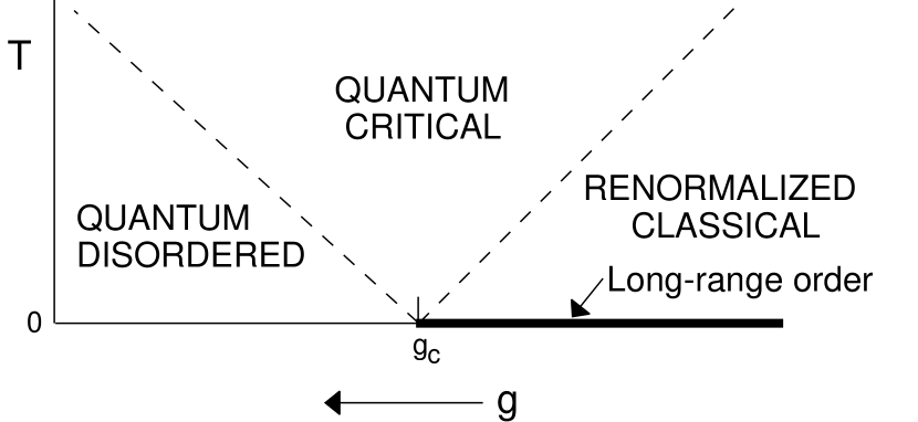
FIG. 1.: Crossover phase diagram for the $d=1$ Ising chain ${\cal H}_{I}$ (Eqn. (1)). The quantum phase transition at $T=0$, $g=g_{c}$ has exponents $z=1$, $\nu=1$. There is true long-range order at $T=0$ for $g<g_{c}$, as indicated by the thick line. The parameter $m\sim g_{c}-g$, so $m=0$ at the critical point and $m>0$ on the ordered side. An essentially identical phase diagram applies to the $d=2$, $O(3)$ quantum rotor model [2, 3], with the difference that the exponents $z=1$, $\nu\approx 0.7$; the crossover phase boundaries, which occur at $|g-g_{c}|^{z\nu}\sim T$, would then not be linear. All regions display critical fluctuations at short scales. In the renormalized-classical and quantum-disordered regions, these cross-over to behavior appropriate to the non-critical ground state before thermal effects have become apparent. In contrast, in the quantum-critical region, the critical fluctuations are quenched in a universal manner by thermal effects, and characteristics of the non-critical ground state do not appear at any scale [3].

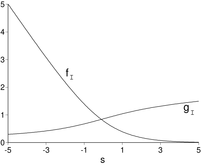
FIG. 2.: The universal crossover functions $f_{I}$ and $g_{I}$ of the Ising model as a function of $s=mc^{2}/k_{B}T$

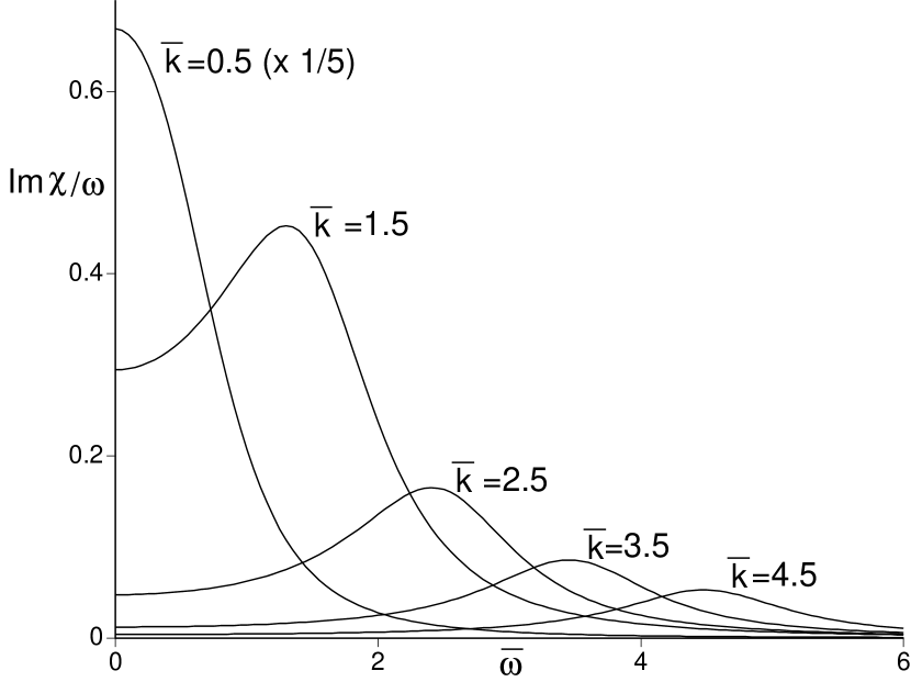
FIG. 3.: The spectral density of the dynamic susceptibility, $\mbox{Im}\chi(k,\omega)/\omega$, of the transverse field Ising model in $d=1$ at its critical coupling $g=g_{c}$ ($m=0$) but with $T$ finite. The scale of the vertical axis is determined by the non-universal constant $Z$ in (21), and has been chosen arbitrarily. We have $\overline{k}=\hbar ck/k_{B}T$, $\overline{\omega}=\hbar\omega/k_{B}T$; the horizontal axis is therefore measured in dimensionless units and its scale is meaningful.

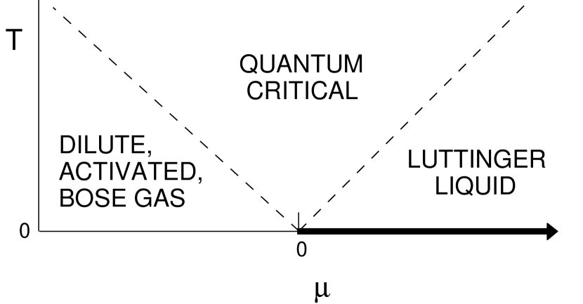
FIG. 4.: Crossover phase diagram for a dilute Bose gas in $d=1$ from Ref [4]. The $T=0$ quantum phase transition occurs at chemical potential $\mu=0$ and has exponents $z=2$, $\nu=1/2$. The temperature $T$ is the most important energy scale in the quantum-critical region. The Luttinger liquid has power-law correlations at $T=0$ (indicated by the thick line), while there is exponential decay at any finite $T$. The same phase diagram applies for $1<d<2$ except that there is true long-range order at $T=0$ on the thick line, and the nomenclature “incipient superfluid” is more appropriate than “Luttinger liquid”.

REFERENCES

- [1] A partial, representative list of references is J.A. Hertz, Phys. Rev. B 14, 525 (1976); A.J. Millis, Phys. Rev. B 48, 7183 (1993); A.M. Tsvelik and M. Reizer, Phys. Rev. B 48, 9887 (1993); S. Sachdev and J. Ye, Phys. Rev. Lett. 69, 2411 (1992); N. Elstner, R.L. Glenister, R.R.P. Singh, and A. Sokol: Phys. Rev. B 51, 8984 (1995); I. Affleck and A.W.W. Ludwig, Nucl. Phys. B360, 641 (1991); I.E. Perakis, C.M. Varma, and A.E. Ruckenstein, Phys. Rev. Lett. 70, 3467 (1993).
- [2] S. Chakravarty, B.I. Halperin, and D.R. Nelson, Phys. Rev. B 39, 2344 (1989).
- [3] A.V. Chubukov, S. Sachdev and J. Ye, Phys. Rev. B 49, 11919 (1994).
- [4] S. Sachdev, T. Senthil, and R. Shankar, Phys. Rev. B 50, 258 (1994); .
- [5] E. Lieb, T. Schultz, and D. Mattis, Ann. of Phys. 16, 406 (1961); P. Pfeuty, Ann. of Phys. 57, 79 (1970); and the review J.B. Kogut, Rev. Mod. Phys. 51, 659 (1979).
- [6] Quantum Inverse Scattering Method and Correlation Functions by V.E. Korepin, N.M. Bogoliubov, and A.G. Izergin, Cambridge University Press, Cambridge (1993) and references therein.
- [7] S. Sachdev in Proceedings of the 19th IUPAP International Conference on Statistical Physics, edited by B.-L. Hao, World Scientific, Singapore, to be published; cond-mat/9508080
- [8] B.M. McCoy, J.H.H. Perk, and R.E. Shrock, Nucl. Phys. B220, 35 (1983); A.R. Its, A.G. Izergin, V.E. Korepin, V.Ju. Novokshenov, Nucl. Phys. B 340, 752 (1990); P. Deift and X. Zhou in Singular Limits of Dispersive Waves, edited by N.M. Ercolani et. al., Plenum Press, New York, 1994 (NATO ASI Series Vol. 320), pp. 183-201.
- [9] J.H.H. Perk, H.W. Capel, G.R.W. Quispel, and F.W. Nijhoff, Physica 123A, 1 (1984).
- [10] H.W. Capel and J.H.H. Perk, Physica 87A, 211 (1977); J.H.H. Perk and H.W. Capel, Physica 89A, 265 (1977).
- [11] B.M. McCoy, Phys. Rev. 173, 531 (1968).
- [12] R.J. Glauber, J. Math. Phys. 4, 294 (1963).
- [13] B.M. McCoy and T.T. Wu, The Two-Dimensional Ising Model, Harvard University Press, Cambridge, U.S.A. (1973).
- [14] T.T. Wu, B.M. McCoy, C.A. Tracy, E. Barouch, Phys. Rev. B 13, 316 (1976).
- [15] Statistical Field Theory by C. Itzykson and J.-M. Drouffe, Cambridge University Press, Cambridge (1989).
- [16] D. Bernard and A. LeClair, Nucl. Phys. B 426, 534 (1994).
- [17] V.E. Korepin and N.A. Slavnov, Commun. Math. Phys. 129, 103 (1990); A.R. Its, A.G. Izergin, V.E. Korepin, Physica D 53, 187 (1991); A.R. Its, A.G. Izergin, V.E. Korepin and G.G. Varzugin, Physica D 54, 351 (1992).
- [18] A. Luther and I. Peschel, Phys. Rev. B 9, 2911 (1974), B 12, 3908 (1975); H.J. Schulz, Phys. Rev. B 34, 6372 (1986); R. Shankar, Int. J. Mod. Phys. B 4, 2371 (1990).
- [19] J.L. Cardy, J. Phys. A 17, L385 (1984).
- [20] M.P.A. Fisher, P.B. Weichmann, G. Grinstein, and D.S. Fisher, Phys. Rev. B 40, 546 (1989).
- [21] O. Babelon and D. Bernard, Physics Letters. B 288, 113 (1992).
- [22] J.L. Cardy and G. Mussardo, Nucl. Phys. B 340, 387 (1990); V.P. Yurov and Al.B. Zamalodchikov, Int. J. Mod. Phys. A 6, 3419 (1991).
- [23] S. Sachdev, unpublished.
- [24] R.V. Jensen and R. Shankar, Phys. Rev. Lett. 54, 1879 (1985).
- [25] E. Barouch and B.M. McCoy, Phys. Rev. A 3, 786 (1971).
- [26] There appears to be a crucial missing prefactor of 1/4 in Eqn (3.28) and subsequent equations of Ref [11]. If omitted, the scaling structure of the results would be spoiled.