Coulomb Blockade in a Quantum Dot Coupled Strongly to a Lead

Abstract

We study theoretically a quantum dot in the quantum Hall regime that is strongly coupled to a single lead via a point contact. We find that even when the transmission through the point contact is perfect, important features of the Coulomb blockade persist. In particular, the tunneling into the dot via a second weakly coupled lead is suppressed, and shows features which can be ascribed to elastic or inelastic cotunneling through the dot. When there is weak backscattering at the point contact, both the tunneling conductance and the differential capacitance are predicted to oscillate as a function of gate voltage. We point out that the dimensionless ratio $\xi$ between the fractional oscillations in $G$ and $C$ is an intrinsic property of the dot, which, in principle, can be measured. We compute $\xi$ within two models of electron-electron interactions. In addition, we discuss the role of additional channels.

]

I Introduction

The Coulomb blockade occurs in an isolated mesoscopic island when the capacitive charging energy to add a single electron suppresses the discrete fluctuations in the island’s charge. [1] In the past several years this physics has been studied extensively in both metallic systems [2] and in semiconductor structures. [3] The Coulomb blockade is most easily probed by measuring transport through an island which is weakly coupled to two leads. By varying a gate voltage $V_{G}$, which controls the chemical potential of the island, peaks in the conductance are observed each time an additional electron is added. Between the peaks, the conductance is activated, reflecting the Coulomb barrier to changing the number of electrons on the dot.

The coupling to the island via tunnel junctions introduces fluctuations on the dot which relax the discreteness of its charge. When the conductance $\sigma$ of the junctions is very small, $\sigma\ll e^{2}/h$, this effect is weak and gives rise to the well known cotunneling effect, in which electrons may tunnel virtually through the Coulomb barrier. [4, 5] Provided one is not too close to a degeneracy between different charge states, this physics may be described satisfactorily within low order perturbation theory in the tunnel coupling.

For stronger coupling to the leads, the perturbative analysis is no longer adequate, and a quantitative description of the problem becomes much more difficult. Based on general arguments, the Coulomb blockade is expected to be suppressed when $\sigma\approx e^{2}/h$, [6] since in that regime, the $RC$ decay time of the island leads to an uncertainty in the energy which exceeds the Coulomb barrier. However, this argument is unable to predict quantitatively the nature of the suppression of the Coulomb blockade.

A particularly well suited system to study this physics is a semiconductor quantum dot at high magnetic fields. In the integer quantum Hall effect regime, the states near the Fermi energy of a quantum dot are edge states, and have a simple, well organized structure, which is insensitive to the complicating effects of impurities and chaotic electron trajectories. In this paper we shall study a quantum dot in the integer quantum Hall regime which is strongly coupled to a lead via a quantum point contact with one (or a few) nearly perfectly transmitting channels.

In a recent paper, Matveev [7] has considered a dot connected to a single lead by a nearly perfectly transmitting point contact. When the transmission of the point contact is perfect (zero backscattering), he showed that even in the presence of a substantial Coulomb energy $U$, the differential capacitance $C=dQ/dV_{G}$ is independent of $V_{G}$. Thus, the equilibrium charge $Q$ on the island is maximally un-quantized, since charge is added continuously as the gate voltage is changed. He then showed that the presence of weak backscattering at the point contact leads to weak oscillations in the differential capacitance as a function of gate voltage with a period corresponding to the addition of a single electron. These oscillations signal the onset of the quantization of the equilibrium charge on the island.

In addition to the capacitance measurements, [7, 8] the fate of the Coulomb blockade in an island connected to a single lead via a point contact can be probed by transport, provided an additional lead is present. This leads us to the interesting possibility of simultaneously measuring the conductance (a transport property) and the capacitance (an equilibrium property) of a quantum dot. In this paper, we build on Matveev’s work and compute, in addition to the differential capacitance, the tunnel conductance and $I$-$V$ characteristics for an island connected to one lead with a nearly perfectly transmitting point contact and connected very weakly to another lead.

Specifically, we consider the quantum dot depicted schematically in Fig. 1. The center region surrounded by the gates forms a quantum dot, which is connected to the leads on both sides. In the $\nu=1$ quantum Hall regime, there is a single edge channel going around the dot. The contact to the left lead is a tunnel junction, characterized by a small tunneling amplitude $t$, which is controlled by the voltage on gate A. The right contact is a nearly perfectly transmitting point contact characterized by a small backscattering amplitude $v$, which is controlled by the voltage on gate B. The backscattering at the point contact involves tunneling of electrons between the opposite moving edge channels at $x=L$ and $x=-L$, where $x$ is a parameter specifying the spatial coordinate along the edge channel.

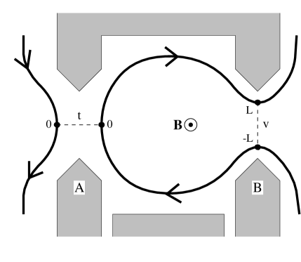
FIG. 1.: Schematic view of a quantum dot connected to leads on both sides. Negative voltage on the gates (shaded area) confines electrons in the dot. Thick solid lines show the edge channels formed by strong magnetic field $B$, where the direction of the electron motion is depicted by arrows. Dashed lines show tunneling paths, where the tunneling amplitude $t$ and the backscattering amplitude $v$ are controlled by voltage on gate A and gate B, respectively.

A crude estimation of the Coulomb energy with the above geometry gives $U=Ke^{2}/\epsilon L$, where $K$ is a dimensionless geometrical factor and $\epsilon$ is the dielectric constant of the semiconductor material. Another geometry-dependent energy scale is the level spacing between edge states in an isolated dot, $\Delta E=\pi\hbar v_{F}/L$. While there are few reliable estimates of the edge state velocity $v_{F}$, the ratio $\Delta E/U$ is typically of the order 0.1 in GaAs/AlGaAs heterostructures in the integer quantum Hall effect regime. [9] The smallness of this ratio is assumed throughout this paper.

Though the equilibrium charge on the dot is not quantized when the transmission at the point contact is perfect, we nonetheless find that important features of the Coulomb blockade remain in the tunneling characteristics. Remarkably, most of these features can be explained within the usual weak coupling model. Specifically, we find that at zero temperature, the Ohmic conductance is suppressed by a factor of $(\Delta E/U)^{2}$ below its noninteracting (i.e. $U=0$) value. This suppression of the tunnel conductance is precisely of the form predicted by the theory of elastic cotunneling through a one dimensional system. Evidently, the cotunneling theory is more general than its derivation within weak coupling perturbation theory suggests. In addition, when the temperature $T$ or the voltage bias $eV$ exceeds $\Delta E$, we find behavior analogous to inelastic cotunneling. In particular, for $\Delta E\ll T\ll U$ the tunneling conductance is suppressed by $(T/U)^{2}$. Moreover, for $\Delta E\ll eV\ll U$, the tunneling current varies as $V^{3}$.

Inelastic cotunneling behavior has also recently been discussed by Furusaki and Matveev [10] for a quantum dot strongly coupled to two leads. While similar in many respects, it is worthwhile to distinguish the present work from that in Ref. [A]. In that reference, the two point contacts are considered to be independent. An electron passing through one contact can never coherently propagate to the second contact. Elastic cotunneling can therefore not be described within that framework. In general, the elastic cotunneling will depend on the complicated transmission matrix of the sample. In contrast, in the quantum Hall regime, the edge channels have a particularly simple structure and directly connect the leads. If the phase coherence length can exceed the dot’s dimensions, then elastic cotunneling should be present. This physics is correctly accounted for in our edge state model. In addition, the beautiful results in Ref. [A] concerning the Coulomb blockade for spin degenerate systems is not applicable here, since the magnetic field destroys that degeneracy.

In addition to the limiting behaviors discussed above, we find that at low temperature $T\ll\Delta E$, there can be nontrivial structure in the $I$-$V$ characteristic for $V\approx\Delta E$. In particular, we find steps in the differential conductance, $dI/dV$ as a function of bias voltage. In the weak coupling limit, the existence of such steps has been discussed by Glattli. [5] They are a consequence of inelastic cotunneling when the many body eigenstates of the quantum dot are discrete. Observation of such steps could provide a new spectroscopy of the low lying many body states of a quantum dot. Remarkably, as we shall show in Sec. III, these steps can remain sharp in the strong coupling limit, even though it becomes meaningless in that limit to speak of discrete single particle states.

When the transmission through the point contact is less than perfect, charge quantization is introduced in the dot. The rigidity of the quantization grows with increasing amplitude of the backscattering at the contact. For weak backscattering, this is reflected in oscillations in the differential capacitance as a function of gate voltage, with an amplitude proportional to the backscattering matrix element $v$. We find that similar oscillations, proportional to $v$, should be present in the conductance. A comparison of these oscillations should therefore provide information about the intrinsic structure of the quantum dot. We focus on the ratio of the fractional oscillations in the conductance to that of the capacitance,

$$\xi={G_{1}/G_{0}\over{C_{1}/C_{0}}}.$$ (1)

$G_{0}$ and $C_{0}$ are the average capacitance and conductance, whereas $G_{1}$ and $C_{1}$ are the amplitudes of the oscillations as a function of gate voltage. By considering the fractional oscillations, $G_{1}/G_{0}$ and $C_{1}/C_{0}$, the dependence on the tunneling matrix element $t$ necessary to measure $G$ and the capacitive lever arm $\eta$ necessary to measure $C$ is eliminated. Moreover, since in the weak backscattering limit both quantities are proportional to $v$, the dependence on $v$ is eliminated by taking their ratio. Thus, $\xi$ measures an intrinsic property of the strongly coupled quantum dot which is independent of the details of the tunneling matrix elements. We have computed $\xi$ within a constant interaction model, in which the Coulomb interaction couples only to the total number of electrons on the dot. We find that $\xi\approx 1.59$ for $T,\Delta E\ll U$, independent of $T$, $\Delta E$ and $U$. More generally, $\xi$ will depend on the specific form of the electron-electron interactions.

With a few modifications, the above considerations can be extended to the case in which there are more than one well transmitted channels. We find that the low bias linear conductance is less suppressed as the number of channels ${\cal N}$ increases. It has been recently shown that the suppression factor becomes $(\Delta E/U)^{2/{\cal N}}$ in a constant interaction model. [11] However, if we take it into considerations that the interaction strength may differ within the same channel and between different channels, we find that the factor still has the form $(\Delta E/U)^{2}$. In addition, the ratio $\xi$ depends sensitively on the form of the electron-electron interactions between different channels on the dot. It is equal to zero if different channels do not interact and grows with increasing strength of the inter-channel interactions. Thus, $\xi$ is a measure of the inter-channel interaction strength.

This paper is organized as follows. In Sec. II, we describe the model and derive the $I$-$V$ characteristic equation. In Sec. III we consider a single channel system with a perfectly transmitting point contact. We compute the current and discuss various features of the result. In Sec. IV, we consider the effect of the weak backscattering to the conductance in connection with the effect to the capacitance. We compute $\xi$ within two specific models of electron-electron interactions. In Sec. V, we generalize the results of Sec. III and Sec. IV to multiple channel systems. Finally, some concluding remarks are given in Sec. VI.

II Edge State Model

We begin in this section by describing our edge state model of a quantum dot strongly coupled to a single lead. Here we will consider the case in which only a single channel is coupled to the lead by a nearly perfectly transmitting point contact. Later, in section V we will consider the case where more than one channel is transmitted.

In the absence of interactions, it is a simple matter to describe this system in terms of the free electron edge state eigenstates. Such a description is inconvenient, however, for describing effects associated with the Coulomb blockade, which are due to the presence of a Coulomb interaction. The bosonization technique, however, allows for an exact description of the low energy physics in the interacting problem. [12]

At energies small compared to the bulk quantum Hall energy gap, the many body eigenstates are long wavelength edge magnetoplasmons. These may be described as fluctuations in the one dimensional edge density, $n(x)$, where $x$ is a coordinate along the edge. Following the usual bosonization procedure, we introduce a field $\phi(x)$, such that $n(x)=\partial_{x}\phi/2\pi$. The Hamiltonian, which describes the compressibility of the edge may then be written,

$$H_{0}=\int dx{v_{F}\over{4\pi}}(\partial_{x}\phi)^{2}.$$ (2)

The dynamics of the edge excitations follow from the Kac Moody commutation relations obeyed by $\phi$,

$$\left[\frac{\partial_{x}\phi(x)}{2\pi},\phi(x^{\prime})\right]=i\delta(x-x^{\prime}).$$ (3)

Using (2) and (3) it may easily be seen that $\partial_{t}n=v_{F}\partial_{x}n$, so that the edge excitations propagate in a single direction at velocity $v_{F}$ along the edge. In this language, the electron creation operator on the edge may be written as $\psi^{\dagger}(x)=e^{i\phi(x)}$.

Equations (2) and (3) are an exact description of a single edge channel of noninteracting electrons. We may easily incorporate interactions into this description. Specifically, we consider a “constant interaction model” in which the Coulomb interaction couples to the total number of electrons $N$ on the dot, which depends on the edge charge between $x=-L$ and $x=L$,

$$N={1\over{2\pi}}[\phi(L)-\phi(-L)].$$ (4)

The self capacitance and the coupling to a nearby gate can then be described by the Hamiltonian,

$$H_{U}+H_{G}={U\over 2}N^{2}+e\eta V_{G}N,$$ (5)

where $\eta$ is a “lever arm” associated with the capacitance coupling to the gate. Since the interaction is still quadratic in the boson fields, it may be treated exactly in this representation.

Now we consider tunneling between the edge channels. We consider the left lead in Fig. 1 to be a Fermi liquid. Without loss of generality, we model it as another $\nu=1$ quantum Hall edge, characterized by a boson field $\phi_{l}$ with a Hamiltonian $H_{0}$ in (2). Tunneling from the left lead into the dot at $x=0$ is then described by the operator

$${\sf T}_{\rightarrow}=\mbox{e}^{i[\phi(0)-\phi_{l}(0)]}\equiv\mbox{e}^{i\theta}.$$ (6)

where we define $\theta\equiv\phi(0)-\phi_{l}(0)$. For the reverse process, ${\sf T}_{\leftarrow}=\exp-i\theta$. The left point contact may be characterized by a tunneling Hamiltonian,

$$H_{t}=t\cos\theta$$ (7)

where $t$ is the tunneling matrix element.

Similarly, tunneling at the right point contact involves transfer of electrons between $x=-L$ and $x=L$. The Hamiltonian describing these processes can be expressed as

$$H_{v}=v\cos[\phi(L)-\phi(-L)]=v\cos 2\pi N,$$ (8)

where $v$ is the backscattering matrix element.

It is convenient to eliminate the linear gate voltage term in (5) by the transformation $N\rightarrow N-N_{0}$, where $N_{0}=e\eta V_{G}/(\Delta E+U)$ is the optimal number of electrons on the dot. Our model Hamiltonian describing a quantum dot with a single channel coupled to a lead may then be written

$$H = H_{0}[\phi_{l}]+H_{0}[\phi]+{U\over 2}N^{2}$$ (10)

$$+t\cos\theta+v\cos 2\pi(N-N_{0}).$$

We will find it useful in our analysis to represent the partition function as an imaginary time path integral. The action corresponding to $H_{0}$ is then given by

$$S_{0}=\frac{1}{4\pi}\int dxd\tau\>\partial_{x}\phi(v_{F}\partial_{x}\phi+i\partial_{\tau}\phi).$$ (11)

Since the remaining terms in the Hamiltonian depend only on $\theta$ and $N$, it is useful to integrate out all of the other degrees of freedom. The resulting action, expressed in terms of $\theta(\tau)$ and $N(\tau)$, is then given by

$$S_{tot} = \frac{1}{2}\sum_{i\omega_{n}}\left[\begin{array}[]{cc}\theta(-\omega_{n})&N(-\omega_{n})\end{array}\right]{\sf G}^{-1}\left[\begin{array}[]{c}\theta(\omega_{n})\\ N(\omega_{n})\end{array}\right]$$ (16)

$$+\int d\tau\left[t\cos\theta+v\cos 2\pi(N-N_{0})\right]$$

where $\omega_{n}$ is a Matsubara frequency. ${\sf G}^{-1}$ is the inverse of the Green’s function matrix and can be explicitly expressed as

$${\sf G}^{-1}={1\over T}\left[\begin{array}[]{cc}\frac{|\omega_{n}|}{4\pi}(1+\mbox{e}^{-\frac{\pi|\omega_{n}|}{\Delta E}})&-\frac{\omega_{n}}{2}\\ \frac{\omega_{n}}{2}&\frac{\pi|\omega_{n}|}{1-\mbox{e}^{-\frac{\pi|\omega_{n}|}{\Delta E}}}+U\end{array}\right],$$ (17)

where $\Delta E\equiv\pi v_{F}/L$.

We now briefly develop the framework for our calculation of the tunneling current. The $I$-$V$ characteristic (or equivalently the tunneling density of states) may be computed using the action $S_{tot}$ in (16). Working perturbatively in the tunneling matrix element $t$, we may compute the tunneling current in the presence of a DC bias $V$ using Fermi’s golden rule.

$$I = \frac{\pi et^{2}}{2\hbar}\sum_{m,n}e^{-E_{m}/kT}\left[\left|\left<n|{\sf T}_{\rightarrow}|m\right>\right|^{2}\delta(E_{n}-E_{m}-eV)\right.$$ (19)

$$\quad\left.-\left|\left<n|{\sf T}_{\leftarrow}|m\right>\right|^{2}\delta(E_{n}-E_{m}+eV)\right],$$

where $\left|m\right>$ is an eigen state of the unperturbed Hamiltonian with energy $E_{m}$. Since the sum on $n$ is over a complete set of states, we can re-express the above equation as

$$I=\frac{\pi et^{2}}{2h}P(eV)$$ (20)

where

$$P(E)=\int dt\>\mbox{e}^{iEt}\left<\left[\mbox{e}^{i\theta(t)},\mbox{e}^{-i\theta(0)}\right]\right>.$$ (21)

In order to compute $P(E)$, it is useful to consider the imaginary time ordered Green’s function, which may be readily computed using path integral techniques.

$${\cal P}(\tau)\equiv\left<\mbox{T}_{\tau}\mbox{e}^{i\theta(\tau)}\mbox{e}^{-i\theta(0)}\right>.$$ (22)

The real time correlation function may then be deduced by analytic continuation. The two terms in the commutater in (21) lead to

$$P(E)=P^{>}(E)-P^{<}(E)$$ (23)

with

$$P^{>,<}(E)=\int dte^{iEt}{\cal P}(\tau\rightarrow it\pm 0^{+})$$ (24)

Limiting behavior of the tunneling current may be deduced analytically from the asymptotic behavior of ${\cal P}(\tau)$. In particular, at zero temperature, the Ohmic conductance is proportional to the coefficient of the $1/\tau^{2}$ term. In addition, it is possible to compute $P(E)$ numerically, as is described in the following section and in more detail in appendix A.

III Point Contact with Perfect Transmission

In this section, we will consider the case where the transmission through the right point contact is perfect. In this limit, there is no quantization of the charge on the dot. Since charge may flow continuously through the point contact, there is no preferred integer value for the charge. This may be seen clearly from the Hamiltonian in equation (10), where for $v=0$ the dependence on $N_{0}$ is absent.

It follows that as the gate voltage is varied that there should be no oscillations in either the differential capacitance or the conductance. However, we will show below that tunneling through a large barrier onto the dot is still blocked by the charging energy. This blockade is a result of the fact that the tunneling electron has a discrete charge, which cannot immediately be screened.

To compute the tunneling current, we evaluate ${\cal P}_{0}(\tau)$, where the subscript $0$ indicates that $v=0$. Since the action (16) is quadratic, we may write,

$${\cal P}_{0}(\tau) = \mbox{e}^{-\frac{1}{2}\left<\mbox{T}_{\tau}\left[\theta(\tau)-\theta(0)\right]^{2}\right>}$$ (25)

$$= \exp\left[-\sum_{\omega_{n}}\left(1-\mbox{e}^{i\omega_{n}\tau}\right){\sf G}_{\theta\theta}\right]$$ (26)

where ${\sf G}_{\theta\theta}$ is the top left element of the matrix ${\sf G}$ defined in (16). This may be rewritten as

$${\cal P}_{0}(\tau)=\left({\pi\tau_{c}/\beta\over{\sin\pi\tau/\beta}}\right)^{2}\exp\left[-2\pi T\sum_{\omega_{n}}(1-e^{i\omega_{n}\tau}){f(\omega_{n})\over|\omega_{n}|}\right]$$ (27)

where $\tau_{c}$ is the short time cutoff (which is of order the inverse of the cyclotron frequency) and

$$f(\omega)=\frac{U\left(1-\mbox{e}^{-\frac{\pi|\omega|}{\Delta E}}\right)^{2}}{2\pi|\omega|+U\left(1-\mbox{e}^{-\frac{2\pi|\omega|}{\Delta E}}\right)}.$$ (28)

The first term in (27) describes the response for noninteracting electrons, $U=0$. This gives us a purely Ohmic tunneling current $I=G_{U=0}V$. $G_{U=0}$ is related to the transmission probability of a free electron through the left barrier, $G_{U=0}=(e^{2}/h)T_{L}$, where $T_{L}\propto t^{2}$.

In the presence of interactions, the low bias linear conductance may be deduced from the long time behavior of ${\cal P}_{0}(\tau)$. In the strong interaction limit, $U\gg\Delta E$, we may estimate the limiting behavior of the exponential factor in (27) by noting that $f(\omega)$ is approximately a constant in each of the following three limits:

$$f(\omega)\approx\left\{\begin{array}[]{ll}0&\mbox{if}\ \omega\ll\Delta E,\\ 1&\mbox{if}\ \Delta E\ll\omega\ll U,\\ 0&\mbox{if}\ U\ll\omega.\\ \end{array}\right.$$ (29)

At zero temperature, we thus have, to logarithmic accuracy,

$${\cal P}_{0}(\tau)\approx\left(\tau_{c}\over\tau\right)^{2}\exp-2\int_{\Delta E}^{U}{d\omega\over\omega}$$ (30)

in the long time limit ($\tau\gg\Delta E^{-1}$). It then follows that the linear conductance is suppressed. Performing the integral in (27) exactly, we find

$$G=c_{1}{e^{2}\over h}T_{L}\left(\Delta E\over U\right)^{2}.$$ (31)

with $c_{1}\approx 3.11$. This should be compared with the theory of elastic cotunneling, which is derived in the case of weak tunneling through both barriers, $T_{L},T_{R}\ll 1$. When the dot is a one dimensional system (as it is for quantum Hall edge states), the result has been shown to be

$$G\propto{e^{2}\over h}T_{L}T_{R}\left({\Delta E\over U}\right)^{2}.$$ (32)

Evidently, the $\Delta E/U$ suppression predicted in (31) remains valid all of the way up to $T_{R}=1$.

At finite temperatures or voltages, $\Delta E\ll eV,T\ll U$, the lower limit of the integral in (30) is cut off by $T$ and $eV$. The resulting tunneling current may thus be obtained by setting $\Delta E=0$ and written,

$$I=c_{2}{e^{2}\over h}T_{L}{(eV)^{2}+4\pi^{2}T^{2}\over U^{2}}V,$$ (33)

with $c_{2}=2\pi^{2}\mbox{e}^{-2\mbox{\bf C}}/3\approx 2.07$ where C is Euler’s constant. This result is, again, exactly in accordance with the theory of inelastic cotunneling, setting $T_{R}=1$.

An alternative interpretation of this suppression of the tunneling current has been pointed out in Ref. [A]. Suppose that an electron tunnels into the dot. The dot would minimize its electrostatic energy by discharging exactly one electron. According to Friedel sum rule, the number of added electrons, which is $-1$ in this case, is equal to $\delta/\pi$ where $\delta$ is the scattering phase shift of the one dimensional channel. As in Anderson orthogonality catastrophe, [14] the suppression factor in the tunneling rate is related to the phase shift by

$${dI\over dV}\propto\varepsilon^{\gamma}$$ (34)

where $\varepsilon=\max(\Delta E,T,eV)$ is the low energy cutoff and

$$\gamma = 2\left(\delta\over\pi\right)^{2}$$ (35)

$$= 2(-1)^{2}=2.$$ (36)

Combining (34) and (36), we may reproduce (31) and (33). Note that (36) differs from the usual orthogonality exponent, $(\delta/\pi)^{2}$, by a factor of two. This is because we are tunneling into the middle of a “chiral” system consisting only of right moving electrons (or equally the end of a one dimensional normal electron gas.)

Finally, we note that in the high bias limit, $eV\gg U$, we recover the linear $I$-$V$ characteristic with an offset characteristic of the Coulomb blockade,

$$I={e^{2}\over h}T_{L}\left(V-{U\over{2e}}\right).$$ (37)

This offset is a consequence of the fact that at short times, the electron which tunnels can not be effectively screened by the point contact.

In addition to the limiting behaviors described above, we have computed the $I$-$V$ characteristic numerically at zero temperature, as explained in appendix A. Fig. 2 shows the differential conductance $dI/dV$. What is most striking is that there are sharp steps whose sizes are approximately $\Delta E$. For a nearly isolated dot, a similar phenomenon has been pointed out by Glattli, [5] and can be understood to be a consequence of inelastic cotunneling through a dot with a discrete energy level spectrum.

FIG. 2.: Differential conductance $dI/dV$ as a function of scaled bias voltage $eV/U$, computed in the absence of backscattering ($T_{R}=1$) for various $\Delta E$. Curves are scaled so that $dI/dV=1$ in the high bias voltage limit. It is easy to see that the curves consist of steps of approximate size $\Delta E$.

An inelastic cotunneling process leaves a particle-hole excitation in the dot. As the bias voltage increases, the number of available particle-hole combinations also increases. Because of the discrete nature of the energy spectrum of the dot, this increase in number occurs discontinuously at every $\Delta E/e$ of the bias voltage, which is manifested in the tunneling density of states or the differential conductance. However, the above explanations are not fully adequate in our model because the dot is strongly coupled to the lead. For perfect transmission, the line width of a single particle energy level is approximately $\Gamma\sim\Delta E$. It means that the levels are as broad as the level spacing and the steps are expected to be wiped out altogether. The reason for the apparent discrepancy is that the lifetime of a many body excited state (i.e. a particle-hole pair) can be much larger than the naive single particle lifetime.

If the dot is weakly coupled to the lead, the lifetime of a particle-hole excitation may be easily calculated. First, we assume the excitation is relaxed only through the process in which both the particle and the hole tunnel out of the dot. In analogy with the theory of cotunneling, [4] we use Fermi’s golden rule to estimate the decay rate,

$$\tau^{-1} = \frac{2\pi}{\hbar}\sum_{k,k^{\prime}}\left|V_{1k}V_{2k^{\prime}}\left[\frac{1}{\epsilon_{k}-(\epsilon_{1}-\frac{U}{2})}+\frac{1}{\epsilon_{2}+\frac{U}{2}-\epsilon_{k^{\prime}}}\right]\right|^{2}$$ (39)

$$\times\delta(\epsilon_{1}-\epsilon_{2}-\epsilon_{k}+\epsilon_{k^{\prime}})\theta(\epsilon_{k}-\mu)\theta(\mu-\epsilon_{k^{\prime}}),$$

where $\mu$ is the chemical potential of the lead and $\epsilon_{1}$ and $\epsilon_{2}$ are the energies of the particle and the hole respectively. The electron eigenstates in the lead are labeled by $k$ and $k^{\prime}$, and $V_{1k}$ and $V_{2k^{\prime}}$ are matrix elements of the coupling Hamiltonian. If $\epsilon_{1}-\epsilon_{2}\ll U/2$, the above equation can be approximated

$$\tau^{-1} = \frac{32\pi}{\hbar}\frac{|V|^{4}}{\Delta_{lead}^{2}}\frac{\epsilon_{1}-\epsilon_{2}}{U^{2}}$$ (40)

$$= \frac{4}{\pi^{2}h}(\epsilon_{1}-\epsilon_{2})\left(\Delta E\over U\right)^{2}T_{R}^{2},$$ (41)

where $\Delta_{lead}$ is the level spacing of the lead and $T_{R}\approx|2\pi V|^{2}/\Delta E\Delta_{lead}$ is the transmission probability. We assume $|V_{1k}|^{2}\approx|V_{2k^{\prime}}|^{2}\approx|V|^{2}$ is constant in the given range.

In our model, a simple consideration of the $I$-$V$ characteristic equation in (20) and (A2) shows that the width of the step risers is proportional to $(\Delta E/U)^{2}$. Since the width of the risers is directly proportional to the line width of the energy levels, it is evident that Eq. (41) is valid even up to $T_{R}=1$ with a possible numerical factor. We thus conclude that even in the presence of a perfectly transmitting contact, there can be long-lived excited states in the dot, whose decay is suppressed by the Coulomb blockade.

So far we have assumed $\Delta E$ is constant. If we allow non-uniform level spacing, degeneracy in the particle-hole excitation energy is lifted and all steps but the first one split into several sub-steps. As the degree of degeneracy increases with the energy, more splittings occur at higher bias voltages, finally making it hard to distinguish between steps.

Before we close this section, let us consider other relaxation processes. It is only when all relaxation rates are less than $\Delta E$ that it is possible to experimentally observe the steps. This criterion is equivalent to saying that the inelastic scattering length, $l_{\phi}$, is much longer than the circumference of the dot. It is known that inelastic scattering is strongly suppressed in the quantum Hall regime [15] most likely due to the difficulty of conserving both energy and momentum when scattering occurs in a one dimensional channel. These steps may thus be observable in the quantum Hall regime.

IV Point Contact with Weak Backscattering

In this section, we consider the case where there is weak backscattering at the right point contact. As the contact is pinched off, fractional charge fluctuations in the dot are hampered and the discreteness of charge becomes important. For weak backscattering $v$, there is an energy cost, proportional to $v$ in the Hamiltonian (8) for non-integral charge configurations. This gives rise to oscillations in physical quantities such as the capacitance and the conductance as a function of gate voltage. The period of these oscillations corresponds to changing the optimal number of electrons on the dot $N_{0}$ by one.

For nearly perfect transmission through the point contact, we thus expect the conductance and the differential capacitance $C=-edN/dV_{G}$ to have the form,

$$C = C_{0}+C_{1}\cos 2\pi N_{0}$$ (42)

$$G = G_{0}+G_{1}\cos 2\pi N_{0},$$ (43)

where the oscillatory components $C_{1}$ and $G_{1}$ are proportional to $v$. An intrinsic quantity, which is independent of the backscattering amplitude $v$, the tunneling matrix element $t$, and the capacitive lever arm $\eta$ associated with the gate, is the ratio

$$\xi\equiv{G_{1}/G_{0}\over{C_{1}/C_{0}}}.$$ (44)

Using the model we have developed so far, we can calculate the capacitance and the linear conductance perturbatively in the backscattering matrix element $v$. The differential capacitance is given by $C=Td^{2}\ln Z/dV_{G}^{2}/\eta$, where $Z$ is the partition function. As shown by Matveev, to leading order in $v$ the differential capacitance has the form (42) with average and oscillatory components given by

$$C_{0} = \frac{\eta e^{2}}{\Delta E+U},$$ (45)

$$C_{1} = v\eta\mbox{e}^{-2\pi^{2}\left<N(0)^{2}\right>_{0}}\left(\frac{2\pi e}{\Delta E+U}\right)^{2}.$$ (46)

The average $\left<\cdots\right>_{0}$ is with respect to the ground state of the unperturbed action $S_{tot}$ in (16).

In order to compute the conductance, we must calculate ${\cal P}(\tau)$ in the presence of the perturbation $v\cos 2\pi(N-N_{0})$. To the first order in $v$, we find that ${\cal P}(\tau)={\cal P}_{0}(\tau)+{\cal P}_{1}(\tau)\cos 2\pi N_{0}$, where ${\cal P}_{0}(\tau)$ is given in (25) and

$${\cal P}_{1}(\tau) = -\left<\mbox{T}_{\tau}\mbox{e}^{i\left[\theta(\tau)-\theta(0)\right]}S_{v}\right>_{0}$$ (48)

$$+\left<\mbox{T}_{\tau}\mbox{e}^{i\left[\theta(\tau)-\theta(0)\right]}\right>_{0}\left<S_{v}\right>_{0}$$

where $S_{v}=\int_{0}^{\beta}d\tau^{\prime}v\cos 2\pi N(\tau^{\prime})$. This may be written as

$${\cal P}_{1}(\tau) = v{\cal P}_{0}(\tau)\mbox{e}^{-2\pi^{2}\left<N(0)^{2}\right>_{0}}$$ (50)

$$\times\int d\tau^{\prime}\>\left\{1-\cosh 2\pi\left[{\sf G}_{\theta N}(\tau-\tau^{\prime})-{\sf G}_{\theta N}(\tau^{\prime})\right]\right\},$$

where ${\sf G}_{\theta N}(\tau)$ is the off diagonal element of the Green’s function defined in (16), which may be computed explicitly using (17).

In order to compute the linear conductance, we must compute the large $\tau$ limit of (LABEL:eq:Ptau1). For $U\tau\gg 1$ ${\sf G}_{\theta N}(\tau)$ decays as $(U\tau)^{-1}$, so that the integral is independent of $\tau$. We thus find

$$G_{1}=vG_{0}\mbox{e}^{-2\pi^{2}\left<N(0)^{2}\right>_{0}}\times 2\int d\tau^{\prime}\left[1-{\rm cosh}2\pi{\sf G}_{\theta N}(\tau^{\prime})\right],$$ (52)

where $G_{0}$ is the zeroth order linear conductance.

Using (45), (46), and (52), we obtain an exact expression for the ratio $\xi$,

$$\xi={\Delta E+U\over{4\pi^{2}}}\times 2\int d\tau^{\prime}\left[1-{\rm cosh}2\pi{\sf G}_{\theta N}(\tau^{\prime})\right].$$ (53)

In the limit $T,\Delta E\ll U$, the integral approaches a finite value which depends only on $U$. In this limit we find

$$\xi\approx 1.59.$$ (54)

The cancellation of input parameters like $v,U,\ \mbox{and}\ \Delta E$ may tempt us to suspect $\xi$ be a universal number being constant for all samples. As will be shown below, however, Eq. (54) is true only within a constant interaction model, in which the dependence of the interaction on the spatial separation is ignored. In order to see how $\xi$ changes with different models, let us consider a more general model whose interaction Hamiltonian is given by

$$H_{U}^{\prime}=\frac{1}{8\pi^{2}}\int dxdx^{\prime}\>\partial_{x}\phi(x)U(x,x^{\prime})\partial_{x}\phi(x^{\prime}).$$ (55)

The constant interaction model is regained by assuming $U(x,x^{\prime})=U$ to be uniform. It is sufficient for our purpose to consider just another example. We can think of a local interaction $U(x,x^{\prime})=2LU\delta(x-x^{\prime})\theta(L-|x|)$, which is certainly an extreme limit to the other direction from the constant interaction model. The appropriate Green’s function is given by

$${\sf G}_{\theta N}(\omega_{n})=\frac{T}{\omega_{n}}\left(1-\mbox{e}^{\frac{\pi|\omega_{n}|}{U}}\right),$$ (56)

and then using (53) we get

$$\xi=1.$$ (57)

Now it is clear that $\xi$ depends on the form of the electron-electron interaction. It is, however, noteworthy that the values of $\xi$ computed in two extreme limits are of the same order of magnitude.

V Multiple Channel Systems

In this section we generalize the considerations in the previous sections to the systems of which right contact (nearly) perfectly transmits more than one channel. As the conductance of the contact increases with the number of well transmitted channels ${\cal N}$, the shorter $RC$ decay time allows a higher uncertainty in the energy of the island. Therefore it is natural to expect that the effect of the Coulomb blockade become weakened in multiple channel systems, which will be confirmed below.

It turns out that most of the qualitative considerations for the single channel systems can directly be applied to multiple channel systems. Similar calculations as in Sec. III show that in the absence of backscattering, the low bias linear conductance is still suppressed below its noninteracting value, although the suppression is less strong if ${\cal N}$ is bigger. On the other hand, there are new features arising from the introduction of additional channels, on which we will focus in this section.

For integer quantum Hall states with $\nu>1$, the edge channels tend to be spatially separated. The tunneling will be dominated by the coupling to the nearest edge channel. As indicated in Fig. 3, this means that the tunneling and backscattering will occur in different channels. Then the Hamiltonian for ${\cal N}$ channels is represented by

$$H = H_{0}[\phi_{l}]+\sum_{i}H_{0}[\phi_{i}]+H_{U}$$ (59)

$$\quad+\ t\cos\theta_{1}+v\cos 2\pi\left(N_{\cal N}-N_{0}\right),$$

where the notation is similar to that in Sec. III with the subscript denoting the channel number except that $\phi_{l}$ is the boson field of the left lead. We have redefined $N_{0}$ as the optimal number of electrons in channel ${\cal N}$ alone, which in general depends on lever arms for all channels.

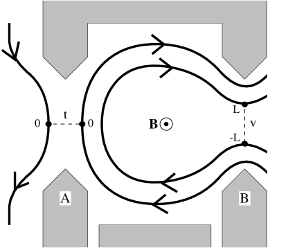
FIG. 3.: Schematic view of a quantum dot analogous to Fig. 1, with two well transmitted channels. The symbols are the same as in Fig. 1. Note that the tunneling through the left contact occurs in the outer channel whereas the backscattering at the right contact occurs in the inner channel.

One of the simplest models to study a multiple channel system is a constant interaction model in which the interaction Hamiltonian depends only on the total charge in the island. The interaction may be explicitly written

$$H_{U}={U\over 2}\left(\sum_{i}N_{i}\right)^{2}.$$ (60)

The calculation of the tunneling conductance proceeds along the same lines as in Sec. III. In this case, the function $f(\omega)$ defined in (27) is given by

$$f(\omega)=\frac{U\left(1-\mbox{e}^{-\frac{\pi|\omega|}{\Delta E}}\right)^{2}}{2\pi|\omega|+{\cal N}U\left(1-\mbox{e}^{-\frac{2\pi|\omega|}{\Delta E}}\right)}.$$ (61)

Note that the limiting values of $f(\omega)$ are

$$f(\omega)\approx\left\{\begin{array}[]{ll}0&\mbox{if}\ \omega\ll\Delta E,\\ \frac{1}{\cal N}&\mbox{if}\ \Delta E\ll\omega\ll{\cal N}U,\\ 0&\mbox{if}\ {\cal N}U\ll\omega.\\ \end{array}\right.$$ (62)

It immediately follows that

$${dI\over{dV}}\propto\frac{e^{2}}{h}T_{L}\left(\frac{\varepsilon}{U}\right)^{2\over{\cal N}},$$ (63)

where $\varepsilon=\max(\Delta E,eV,T)$. The exponent $2/{\cal N}$ has been derived in some other papers in several different contexts. [11, 13] It is clear from (63) that the conductance is less suppressed if there are more channels.

However, it turns out that the nonanalytic behavior with exponent $2/{\cal N}$ is correct only to the extent that the constant interaction model is valid. As explained below, this is due to a special symmetry of the charging energy with respect to redistribution of charge among the different channels. We consider an effective-capacitance model which is one step more general and has been introduced and developed by several authors to remedy some problems with the constant interaction model. [16] This model assumes that the edge channels are capacitively coupled metal bodies and the Coulomb interaction energy depends on the number of electrons in each channel. The Coulomb interaction part of the new Hamiltonian can be written

$$H_{U}=\frac{1}{2}\sum_{ij}N_{i}{\sf U}_{ij}N_{j},$$ (64)

where ${\sf U}$ is an ${\cal N}\times{\cal N}$ matrix which can be determined experimentally. In order to get a clear understanding of the effect of this generalization, let us consider a simple specific example of the electron-electron interaction, i.e.,

$${\sf U}_{ij}=u[{\cal N}a\delta_{ij}+(1-a)].$$ (65)

The diagonal component $({\cal N}a+1-a)u$ is the magnitude of the interaction strength within each channel and the off-diagonal component $(1-a)u$ is that between different channels. This matrix is chosen such that if the lever arms are all equal to unity, the total capacitance $C_{tot}\equiv dQ_{tot}/dV_{G}=e^{2}\sum_{ij}{\sf U}_{ij}^{-1}=e^{2}/u$ in the limit $\Delta E=0$, independent of $a$. Note that we regain a constant interaction model if $a=0$. As $a$ grows we move away from the model, finally reaching an independent channel model at $a=1$, where different channels do not interact. As in (29), the limiting behavior of $f(\omega)$ defined in (27) is given by

$$f(\omega)\approx\left\{\begin{array}[]{ll}0&\mbox{if}\ \omega\ll\Delta E,\\ 1&\mbox{if}\ \Delta E\ll\omega\ll{\cal N}au,\\ \frac{{\cal N}a+1-a}{\cal N}&\mit{\cal N}au\ll\omega\ll{\cal N}u,\\ 0&\mbox{if}\ {\cal N}u\ll\omega,\\ \end{array}\right.$$ (66)

It is clear from the above equation that if $a\rightarrow 0$ (constant interaction), (62) is restored and we get the exponent $2/{\cal N}$, as we discussed earlier. When $a$ is not small, there is no appreciable range in which $f(\omega)=1/{\cal N}$, and the differential conductance has a different exponent, 2, i.e.

$${dI\over{dV}}\propto\frac{e^{2}}{h}T_{L}\left(\varepsilon\over u\right)^{2}$$ (67)

provided $\varepsilon=\max(\Delta E,eV,T)\ll{\cal N}au$.

The above considerations can be generalized to a model with a generic matrix ${\sf U}$. Even though $f(\omega)$ is a complicated function which depends on all matrix elements of ${\sf U}$, there exists an energy scale $\tilde{u}$ which corresponds to $au$ in the above special model, such that

$$f(\omega)\approx 1\quad\mbox{if}\ \Delta E\ll\omega\ll{\cal N}\tilde{u}.$$ (68)

Then Eq. (67) is valid if $\varepsilon\ll{\cal N}\tilde{u}$, except for the factor depending on $a$. In general, $\tilde{u}=0$ for a constant interaction model and it measures how far the used model is away from the constant interaction model. Van der Vaart et al.[18] have measured the matrix elements of ${\sf U}$ for two Landau levels confined in a quantum dot. Even though both contacts were nearly pinched off in the reference as opposed to our model, it is suggestive to estimate the magnitude of $\tilde{u}$ using the experimental data. With their particular setup, they got ${\sf U}_{11}=800$, ${\sf U}_{22}=1175$, and ${\sf U}_{12}=650$ (all in $\mu eV$). A simple estimation with these numbers gives ${\cal N}\tilde{u}\sim 260\mu eV\gg\Delta E,T,eV$, which suggests that (67) must be used rather than (63) in this case. It has to be admitted that this is a naive estimation considering the difference between their experimental setup and our theoretical model. Opening up a point contact would in general reduce the strength of electron-electron interactioins in the dot and it would change the capacitance appreciably. However, even though the above estimation of $\tilde{u}$ may be merely speculative at its best, we expect (67) has to be true if different channels are weakly coupled, which seems more general than the constant interaction limit, in practice.

It is now evident that the exponent is $2/{\cal N}$ only for the constant interaction model. This is due to a special symmetry of the constant interaction model, i.e., the interaction part of the Hamiltonian (59) is invariant under redistribution of total charge among the different channels. The effect of the symmetry to the exponent can be most easily understood in terms of Anderson orthogonality catastrophe. [13] Eq. (34) can be directly used with an appropriately generalized definition of $\gamma$, i.e.,

$$\gamma=2\sum_{i}\left(\delta_{i}\over\pi\right)^{2},$$ (69)

where $\delta_{i}$ is the phase shift in channel $i$. It needs only a little consideration of electrostatics to figure out $\delta_{i}$. Following the argument in Sec. III, let us suppose that an electron has just tunneled into channel 1 through the left contact. The number of electrons discharged from each channel $-\delta_{i}/\pi$ depends on the form of the interaction, provided they satisfy the constraint $\sum\delta_{i}/\pi=-1$. If we work in a constant interaction model, because the Hamiltonian depends only on the total charge, from the symmetry $\delta_{i}/\pi=-1/{\cal N}$ for all $i$. Therefore

$$\gamma=2\sum_{i=1}^{\cal N}\left(-\frac{1}{\cal N}\right)^{2}=\frac{2}{\cal N}.$$ (70)

On the other hand, if we use an effective-capacitance model and the system is safely away from the constant interaction limit (${\cal N}\tilde{u}\gg\Delta E$), it is always energetically favorable to take a whole electron from channel 1 and have the exactly same ground state charge configuration as before. Then $\delta_{1}/\pi=-1$ and $\delta_{i}=0\ (i=2\ldots{\cal N})$, so that

$$\gamma=2(-1)^{2}=2.$$ (71)

Then Eqs. (67) and (63) are readily reproduced from (34) and (69). The physical distinction between the energy scales $u$ and $\tilde{u}$ is thus clear. When an electron is added to the dot, $({\cal N}u)^{-1}$, which corresponds to the $RC$ decay time, sets the time scale for the total charge of the dot to return to its original value. However, even after the total charge has been screened, there may be some imbalance in the distribution of charge between the channels. $({\cal N}\tilde{u})^{-1}$ sets the scale for the relaxation of this imbalance. In the constant interaction model, there is no Coulomb energy cost for such an imbalance, so $\tilde{u}\rightarrow 0$.

Now let us consider the effect of weak backscattering. As in a single channel model, the introduction of weak backscattering $v$ results in oscillations in the capacitance and the conductance. However, an important difference arises from the fact that the tunneling and backscattering occur in different channels.

It has been shown both theoretically [16] and experimentally [17] that the period of the conductance and the capacitance oscillations increases with increasing number of well transmitted channels. This is because the oscillations arise only from the quantization of $N_{\cal N}$, the number of electrons in the backscattered channel. When there are many perfectly transmitting channels, many electrons must be added to the dot to increase $N_{\cal N}$ by 1.

The analysis of the amplitude of the oscillations is a little more complicated. We will again focus on the ratio $\xi$ defined in (44), using the model interaction in (65). We assume $\Delta E,T\ll{\cal N}au$ and all lever arms are taken to be unity. One may include the lever arms explicitly, but it does not change the result qualitatively. Along the same lines as in Sec. IV, the fractional capacitance oscillation may be written

$$\frac{C_{1}}{C_{0}}=v\mbox{e}^{-2\pi^{2}\left<N_{\cal N}(0)^{2}\right>_{0}}\left(\frac{2\pi}{\cal N}\right)^{2}\frac{1}{u}.$$ (72)

The fractional conductance oscillation may also be written

$$G_{1}=vG_{0}\mbox{e}^{-2\pi^{2}\left<N_{\cal N}(0)^{2}\right>_{0}}\times 2\int d\tau^{\prime}\left[1-{\rm cosh}2\pi{\sf G}_{\theta N}(\tau^{\prime})\right],$$ (73)

where the Green’s function is given by

$${\sf G}_{\theta N}(\tau) = \left<\mbox{T}_{\tau}\theta_{1}(\tau)N_{\cal N}(0)\right>$$ (74)

$$= -\int d\omega_{n}\>\mbox{e}^{-i\omega_{n}\tau}$$ (76)

$$\times\frac{(1-a)u\>\mbox{sgn}(\omega_{n})}{(2\pi|\omega_{n}|+{\cal N}au)(2\pi|\omega_{n}|+{\cal N}u)}.$$

We may easily compute ${\sf G}_{\theta N}(\tau)$ in several limits, namely,

$${\sf G}_{\theta N}(\tau)\approx\left\{\begin{array}[]{ll}0&\mbox{if}\ \tau=0,\\ -i\frac{\pi(1-a)}{\cal N}&\mbox{if}\ \frac{2\pi}{{\cal N}u}\ll\tau\ll\frac{2\pi}{{\cal N}au},\\ 0&\mbox{if}\ \tau\rightarrow\infty,\\ \end{array}\right.$$ (77)

and it is monotonically interpolated in between. The above equation is not helpful if $a\sim 1$, but it is sufficient for our purpose which is to see how $\xi$ changes as the system moves away from the constant interaction limit. Since ${\sf G}_{\theta N}(\tau)$ measures the response of $N_{\cal N}$, a period of time $\tau$ after an electron is added into channel 1, the physical interpretation of the above limiting behavior is clear. It takes a time period of order $2\pi/{\cal N}u$ for the total charge of the dot to return to its original value. Channel ${\cal N}$ contributes to this process by discharging $(1-a)/{\cal N}$ of an electron, which can be read from the second line of (77). The reason it is proportional to $1-a$ is that the inter-channel interaction strength is proportional to $1-a$. After a time period of order $2\pi/{\cal N}au$, the charge in each channel returns to its original value, which is reflected in the vanishing ${\sf G}_{\theta N}(\tau)$ in the long time limit. In order to estimate the integral in (73), we may make a crude approximation by substituting a square function for ${\sf G}_{\theta N}(\tau)$, i.e., ${\sf G}_{\theta N}(\tau)=-i\pi(1-a)/{\cal N}$ if $\frac{2\pi}{{\cal N}u}<\tau<\frac{2\pi}{{\cal N}au}$, and ${\sf G}_{\theta N}(\tau)=0$ otherwise. Then we get

$$\frac{G_{1}}{G_{0}}\approx v\mbox{e}^{-2\pi^{2}\left<N_{\cal N}(0)^{2}\right>_{0}}\frac{8\pi(1-a)}{{\cal N}au}\sin^{2}\frac{\pi(1-a)}{2{\cal N}},$$ (78)

and finally

$$\xi\approx\frac{2{\cal N}}{\pi}\frac{1-a}{a}\sin^{2}\frac{\pi(1-a)}{2{\cal N}}.$$ (79)

This is a good approximation if $a\ll 1$. This is a monotonically decreasing function of $a$ and as is explained below, it is a consequence of the fact that the tunneling and the backscattering occur in different channels. A bigger $a$ implies weaker inter-channel interactions and consequently a weaker effect of the backscattering to the conductance. At $a=1$ (independent channels), we cannot use the above equation, but we know that the conductance oscillation would eventually vanish because the backscattering potential does not affect the conductance at all, and therefore $\xi=0$. At $a=0$, (constant interaction) $G_{1}/G_{0}$ diverges, and so does $\xi$. It is because $G_{1}/G_{0}$ diverges as $(u/\varepsilon)^{\frac{1}{\cal N}}$ if the low energy cutoff $\varepsilon$ is small, suggesting that the perturbation theory break down. Without detailed calculations, one might have been able to infer it from the following physical argument. In a constant interaction model, the total number of electrons in the dot $\sum_{i}N_{i}$ is the only gapped mode and there are ${\cal N}-1$ combinations of $N_{i}$ whose fluctuations are not bounded, leading to divergences in individual terms in the perturbation expansion. Therefore, we need to sum up all higher order terms in order to obtain a correct result. In a series of recent papers, Matveev and Furusaki [7, 10] have calculated both the conductance and the capacitance oscillations nonperturbatively in a spin-degenerate two-channel model, which they related to the multichannel Kondo problem. Their calculations show that the oscillations are no longer sinusoidal and the period becomes ${\cal N}$ times smaller so that the maximum occurs each time an electron is added to the dot as a whole (not channel ${\cal N}$ alone). Such results, however, clearly apply only in the case where the degeneracy is guaranteed by a symmetry and hence should not apply in this quantum Hall system.

Without qualitative changes, the above considerations can be generalized to an effective-capacitance model with a generic matrix ${\sf U}$. As in the discussions of the differential conductance $dI/dV$ earlier in this section, an energy scale $\tilde{u}$, which plays the role of $au$, can be determined from the given matrix ${\sf U}$. In most real situations of quantum Hall effect edge channels, $\xi$ is a finite quantity which can be numerically calculated in the effective-capacitance model if all matrix elements of ${\sf U}$ are known.

VI Conclusions

In this paper we have shown that characteristics of the Coulomb blockade, which are normally associated with the weak coupling limit, persist to strong coupling to a lead via a single channel point contact. In particular, (i) we find the analogies of elastic and inelastic cotunneling in the $(\varepsilon/U)^{2}$ suppression of the tunnel conductance. (ii) We find that particle-hole excitations on the dot can acquire a long lifetime due to a “Coulomb blockade” to relaxation. This in principle could lead to observable steps in the low bias differential conductances as a function of bias voltage. (iii) The high bias behavior of the $I$-$V$ characteristic has an offset, indicating the presence of a Coulomb gap. We find similar conclusions when multiple channels are transmitted through the contact, though the suppression of the Ohmic conductance is reduced. In the special case of the constant interaction model, when there is no penalty towards redistribution of charge between the channels, the exponent of the suppression is modified $(\varepsilon/U)^{2\over{\cal N}}$.

When the transmission through the point contact is less then perfect, the oscillations in the conductance and the capacitance may be characterized by the dimensionless ratio $\xi$. While $\xi$ is independent of the tunneling matrix elements, it depends on the precise form of the Coulomb interactions. For a single channel, we have computed it for two different forms of the interaction, and its value is of order unity. For multiple transmitted channels, its value depends even more sensitively on the inter-channel interactions, which is zero when different channels are independent, and grows with increasing strength of the inter-channel interactions.

A Integral Equation for $P_{0}^{>}(\omega)$

In this appendix, we will use Minnhagen’s integral equation [19] method to compute the spectral density function $P_{0}(E)$ for the perfect transmission case. Functions will be given the subscript $0$ to explicitly show that they are calculated in the absence of backscattering. The calculation of the imaginary time Green function ${\cal P}_{0}(\tau)$ is straightforward from (26), and by analytically continuing it we get

$$P_{0}^{>}(t) = {\cal P}_{0}(\tau\rightarrow it+0^{+})$$ (A1)

$$= \mbox{e}^{-\left<\theta(0)^{2}\right>_{0}}\exp\int_{0}^{\infty}d\omega\>\frac{\alpha(\omega)}{\omega}\mbox{e}^{-i\omega t},$$ (A2)

where the average $\left<\cdots\right>_{0}$ is evaluated over the unperturbed action ($t=v=0$). The function $\alpha(\omega)$ is defined

$$\alpha(\omega) \equiv \frac{\omega}{2\pi}\int dt\>\mbox{e}^{i\omega t}\left<\theta(t)\theta(0)\right>_{0}$$ (A3)

$$= i\frac{\omega}{2\pi}\left[\left.\left<|\theta(\omega_{n})|^{2}\right>_{0}\right|_{|\omega_{n}|\rightarrow i\omega}-\left.\left<|\theta(\omega_{n})|^{2}\right>_{0}\right|_{|\omega_{n}|\rightarrow-i\omega}\right]$$ (A4)

$$= 2+\frac{2\frac{U}{\pi\omega}\sin\frac{\pi\omega}{\Delta E}\left(1-\cos\frac{\pi\omega}{\Delta E}\right)}{\left(1+\frac{U}{\pi\omega}\sin\frac{\pi\omega}{\Delta E}\right)^{2}-2\frac{U}{\pi\omega}\sin\frac{\pi\omega}{\Delta E}\left(1-\cos\frac{\pi\omega}{\Delta E}\right)}.$$ (A5)

Now we differentiate (A2) with respect to $t$ and Fourier transform it. Then we finally get an integral equation

$$\omega P_{0}^{>}(\omega)=\int_{0}^{\omega}d\omega^{\prime}\>\alpha(\omega^{\prime})P_{0}^{>}(\omega-\omega^{\prime}).$$ (A7)

We have replaced the upper limit of the original integral $\infty$ with $\omega$ because $P_{0}^{>}(\omega)=0$ for negative $\omega$ at zero temperature.

We now solve the above equation numerically following the procedures described below. We partition the frequency space into equal parts with step size $\Delta\omega\ll\Delta E$ using division points $\omega_{i}$. Then the function $P_{0}^{>}(\omega)$ is replaced by an array of numbers $P_{0}^{>}(\omega_{i})$ and the above integral equation by a matrix equation. Instead of inverting a huge matrix, we may calculate $P_{0}^{>}(\omega_{i})$ by solving an elementary first order algebraic equation if we know $P_{0}^{>}(\omega_{j})$ for all $\omega_{j}<\omega_{i}$. Since we know $P_{0}^{>}(\omega)\propto\omega$ in the low frequency limit where $\omega\ll\Delta E$, (see Sec. III) we may use a linear function in a small low frequency range as a ‘seed’ to start sequential calculations of the rest of the whole range of interest. Note that we cannot determine a multiplicative overall constant in computing $P_{0}^{>}(\omega)$ because the integral equation is homogeneous.

REFERENCES

- [1] For a review, see: Single Charge Tunneling, eds. H. Grabert and M. Devoret (Plenum, New York, 1992).
- [2] D. V. Averin and K. K. Likharev, in: Quantum Effects in Small Disordered Systems, eds. B. Altshuler, P. Lee and R. Webb (North-Holland, Amsterdam, 1990).
- [3] J. H. F. Scott-Thomas, S. B. Field, M. A. Kastner, H. I. Smith, and D. A. Antoniadis, Phys. Rev. Lett. 62, 583 (1989); H. van Houten and C. W. J. Beenakker, Phys. Rev. Lett. 63, 1893 (1989); U. Meirav, M. A. Kastner, and S. J. Wind, Phys. Rev. Lett. 65, 771 (1990).
- [4] D. V. Averin and Yu. V. Nazarov, in: Single Charge Tunneling, eds. H. Grabert and M. Devoret (Plenum, New York, 1992); D. V. Averin and Yu. V. Nazarov, Phys. Rev. Lett. 65, 2446 (1990).
- [5] D. C. Glattli, Physica B 189, 88 (1993).
- [6] G. Falci, G. Schön, and G. T. Zimanyi, Phys. Rev. Lett. 74, 3257 (1995), and references therein.
- [7] K. A. Matveev, Phys. Rev. B 51, 1743 (1995).
- [8] R. C. Ashoori, H. L. Störmer, J. S. Weiner, L. N. Pfeiffer, S. J. Pearton, K. W. Baldwin, and K. W. West, Phys. Rev. Lett. 68, 3088 (1992).
- [9] N. C. van der Vaart, A. T. Johnson, L. P. Kouwenhoven, D. J. Maas, W. de Jong, M. P. de Ruyter van Steneninck, A. van der Enden, and C. J. P. M. Harmans, Physica B 189, 99 (1993).
- [10] A. Furusaki and K. A. Matveev, Phys. Rev. Lett. 75, 709 (1995); A. Furusaki and K. A. Matveev, cond-mat/9508018.
- [11] K. Flensberg, Phys. Rev. B 48, 11156 (1993).
- [12] F. D. M. Haldane, J. Phys. C 14, 2585 (1981); C. L. Kane and M. P. A. Fisher, Phys. Rev. B 46, 15233 (1992).
- [13] K. A. Matveev, L. I. Glazman, and H. U. Baranger, cond-mat/9504099.
- [14] P. W. Anderson, Phys. Rev. Lett. 18, 1049 (1967); K. D. Schotte and U. Schotte, Phys. Rev. 182, 479 (1969).
- [15] J. Liu, W. X. Gao, K. Ismail, K. Y. Lee, J. M. Hong, and S. Washburn, Phys. Rev. B 50, 17383 (1994).
- [16] J. M. Kinaret and N. S. Wingreen, Phys. Rev. B 48, 11113 (1993); P. L. McEuen, N. S. Wingreen, E. B. Foxman, J. Kinaret, U. Meirav, M. A. Kastner, and Y. Meir, Physica B 189, 70 (1993).
- [17] B. W. Alphenaar, A. A. M. Staring, H. van Houten, M. A. A. Mabesoone, O. J. A. Buyk, and C. T. Foxon, Phys. Rev. B 46, 7236 (1992); B. W. Alphenaar, A. A. M. Staring, H. van Houten, I. K. Marmorkos, C. W. J. Beenakker, and C. T. Foxon, Physica B 189, 80 (1993).
- [18] N. C. van der Vaart, M. P. de Ruyter van Steneninck, L. P. Kouwenhoven, A. T. Johnson, Y. V. Nazarov, C. J. P. M. Harmans, and C. T. Foxon, Phys. Rev. Lett. 73, 320 (1994).
- [19] P. Minnhagen, Phys. Lett. 56A, 327 (1976).