Large-scale Simulation of the Two-dimensional Kinetic Ising Model

Abstract

We present Monte Carlo simulation results for the dynamical critical exponent $z$ of the two-dimensional kinetic Ising model using a lattice of size $10^{6}\times 10^{6}$ spins. We used Glauber as well as Metropolis dynamics. The $z$-value of $2.16\pm 0.005$ was calculated from the magnetization and energy relaxation from an ordered state towards the equilibrium state at $T_{c}$.

submitted to Physica A

The precise numerical value of the dynamical critical exponent $z$, which characterizes the critical slowing down at a second-order phase-transition [1], has not been conclusively calculated. This note presents an effort to calculate the value of $z$ using a system of unprecedented size.

In simulations specific attention has been given to calculate $z$ for the Ising model because of its simplicity and its model character as a representant for a universality class. The Ising model is defined by the Hamiltonian

$${\cal H}_{\mbox{\scriptsize Ising}}(s)=-J\sum_{<ij>}s_{i}s_{j}\qquad,\qquad s_{i}=\pm 1$$ (1)

where $\left<ij\right>$ are nearest-neighbour pairs of lattice sites. The exchange coupling $J$ is restricted to be positive (ferro-magnetic).

The dynamics of the system is specified by the transition probability of the Markov chain which will be realized by a Monte Carlo algorithm [3, 4, 5]. We used two transition probabilities

• Metropolis $P(s_{i}\rightarrow s_{i}^{\prime})=\min\{1,\exp\{-\Delta E)\}$

• Glauber $P(s_{i}\rightarrow s_{i}^{\prime})=\frac{1}{2}\{1-s_{i}\tanh(E_{i}/k_{b}T)\},\qquad E_{i}=J\sum_{<i,j>}s_{j}$

Time $t$ in this context is measured in Monte Carlo steps per spin. One Monte Carlo step (MCS) per lattice site, i.e. one sweep through the entire lattice comprises one time unit. Neither magnetization nor energy are preserved in the model.

Our system size, on which the analysis will be based on, was $10^{6}\times 10^{6}$. A new algorithm [9] was employed to simulate this very large lattice. Basically, instead of storing one lattice configuration and iterating in time we store only part of the lattice configuration at all time steps and iterate through the lattice. Thus we were able to reduce the memory requirements from approximately 100 GB to 20 MB.

It is generally believed that one can calculate $z$ from the relaxation into equilibrium. In the theory of dynamical critical phenomena [10], critical slowing down is expressed as the divergence of the linear relaxation time $\tau_{M}^{(l)}$ of the order parameter $M$ (the magnetization) as one approaches criticality ($\theta\rightarrow 0^{+}$ with $\theta=\left(T-T_{c}\right)/T_{c}$)

$$\tau_{M}^{(l)}\sim\theta^{-\nu z},$$ (2)

where $\sim$ stands for asymptotic proportionality and $\nu$ is the static critical exponent of the correlation length $\xi$. The exponent $z$ is called the dynamical critical exponent. In analogy with finite-size scaling in the theory of static critical phenomena one may infer the following finite-size scaling relation for the linear relaxation time

$$\tau_{M}^{(l)}\sim L^{z}\tilde{f}(\theta L^{\frac{1}{\nu}}),$$ (3)

where $\tilde{f}(z^{\prime})$ is a scaling function regular at $z^{\prime}=0$. Relation (3) is valid for $L\gg 1$ and $\theta\ll 1$.

A value for $z$ can be obtained for very large system sizes from the relaxation of the magnetization into equilibrium from another equilibrium state [2]. If the system size tends to infinity and we are at criticality, the above scaling relaxation implies

$$M(t)\sim t^{-\beta/\nu z}\quad.$$ (4)

For the two-dimensional Ising model, the static critical exponents $\beta=1/8$ and $\nu=1$ as well as the critical temperature $T_{c}=1/(\frac{1}{2}\log(1+\sqrt{2}))$ are exactly known.

Two independent calculations were carried out by groups from Heidelberg using Metropolis dynamics and checkerboard updates and Cologne using Glauber dynamics and typewriter update.

Results from the Heidelberg group       During the course of our simulation we have monitored the magnetization $M=(1/L^{2})\sum s_{i}$ as a function of the number of sweeps $t$ (MCS) through the lattice. We averaged over two independent configurations (cf. implementation of the algorithm in [9]). Table 1 shows the raw data.

To determine the value of $z$ from our data we calculated the slope in a log-log plot using

$$\frac{1}{z_{i}}=-8\frac{\log(m_{i})-\log(m_{i-1})}{\log(i)-\log(i-1)}$$

and grouped data points for a linear least-square fit. Plotted in figure 1 is the slope and the first and second order intercepts of the linear fits to these slopes for $1/t\rightarrow 0$ against the inverse time. We obtain a value of $z\approx 2.15\pm 0.02$. This value is in agreement with results from recent series expansion calculations [11, 12], damage spreading simulations [13] as well as other large scale simulates [6, 7].

Results from the Cologne group       Shocked by the huge lattices from the Heidelberg group, we slightly modified and adapted the step method presented in [9] to typewriter update, which was used in our previous calculations with full lattice storage [8]. The use of typewriter update instead of checkerboard update used by the Heidelberg group, simplified this method considerable. Thereby and with optimization techniques similar to multi-spin coding our program reached 3.8 MUpdate/s on an IBM RS6000/990 (Power/2). With this program we calculated 50 iterations of a $10^{6}\times 10^{6}$ lattice on an 8 processor IBM SP1 (Glauber dynamic, user time 31 days). Beside the magnetization the energy was obtained as well. Table 2 shows the data.

Similar to the magnetization one can also calculate the exponent $z$ from the relaxation of the energy [7]:

$$E(t)-E_{\mbox{\scriptsize critical}}\sim t^{-(1-\alpha)/\nu z}=t^{-1/z}\quad{\rm(in~{}two~{}dimensions)}$$ (5)

For the determination of the value of $z$ we calculated an arithmetic mean value of some data points. The number of gathered data points is calculated by $\lceil{\rm iteration}/5\rceil$ Figure 2 shows this and the first order intercepts. The magnetization data $z_{\mbox{\scriptsize Mag}}$ as well as the energy data $z_{\mbox{\scriptsize Energy}}$ lead to a z-value of 2.16 $\pm$ 0.005 for $1/t\rightarrow 0$.

T	$m_{1}$ (Metropolis)	$m_{2}$ (Metropolis)
0	1.00000000	1.00000000
1	0.92097430	0.92097417
2	0.86321233	0.86321220
3	0.83255023	0.83255007
4	0.81309636	0.81309770
5	0.79918281	0.79918239
6	0.78845203	0.78845225
7	0.77976347	0.77976351
8	0.77248408	0.77248426
9	0.76623362	0.76623401
10	0.76076646	0.76076750

Table 1: Raw data for the calculation from the Heidelberg group.

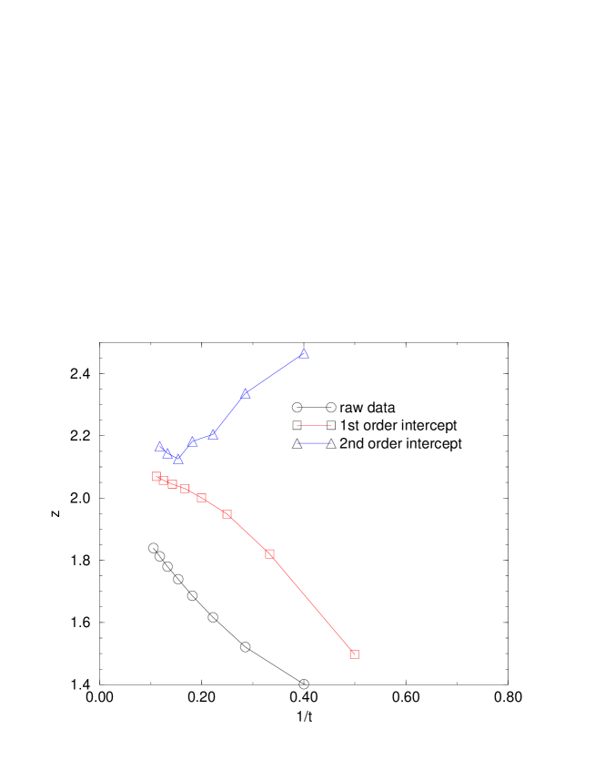
Figure 1: Plot of the critical exponent $z$ vs. $1/t$ (Heidelberg group).

T	m (Glauber)	e (Glauber)	T	m (Glauber)	e (Glauber)	T	m (Glauber)	e (Glauber)
0	1.00000000	0.00000000	17	0.78287989	0.49666620	34	0.75161947	0.52225099
1	0.92387181	0.07612802	18	0.78024367	0.49915815	35	0.75034603	0.52312965
2	0.88930745	0.27878672	19	0.77775922	0.50144418	36	0.74910920	0.52396988
3	0.86826671	0.35298481	20	0.77541236	0.50355210	37	0.74790926	0.52477812
4	0.85343942	0.39143993	21	0.77318752	0.50550180	38	0.74674372	0.52555236
5	0.84208738	0.41546570	22	0.77107242	0.50731384	39	0.74561180	0.52629785
6	0.83292949	0.43221206	23	0.76905750	0.50900323	40	0.74450920	0.52701310
7	0.82527573	0.44472865	24	0.76713498	0.51058358	41	0.74343671	0.52770277
8	0.81871664	0.45453473	25	0.76529694	0.51206432	42	0.74238953	0.52836585
9	0.81298342	0.46248268	26	0.76353643	0.51345741	43	0.74136891	0.52900757
10	0.80789697	0.46910024	27	0.76184711	0.51476957	44	0.74037224	0.52962886
11	0.80333031	0.47472005	28	0.76022277	0.51601052	45	0.73940143	0.53022785
12	0.79918884	0.47957117	29	0.75865931	0.51718485	46	0.73845357	0.53080592
13	0.79540222	0.48381554	30	0.75715202	0.51830041	47	0.73752722	0.53136430
14	0.79191812	0.48756875	31	0.75569749	0.51936114	48	0.73662030	0.53190743
15	0.78869300	0.49091859	32	0.75429320	0.52036977	49	0.73573540	0.53243573
16	0.78568804	0.49393126	33	0.75293487	0.52133128	50	0.73486859	0.53294310

Table 2: Raw data for the calculation by the Cologne group.

Figure 2: Plot of the critical exponent $z$ vs. $1/t$ (Cologne group).

Acknowledgment       Partial support from the BMFT project 0326657D and EU project CPACT 930105 (PL296476) is gratefully acknowledged. Part of this work was funded by a Stipendium of the Graduiertenkolleg “Modellierung und Wissenschaftliches Rechnen in Mathematik und Naturwissenschaften” at the IWR Heidelberg.

We thank D. Stauffer for numerous fruitful discussions and scientific advice. We thank the Leibniz Supercomputing Center Munich for the generous grant of computation time at the local IBM 9076 SP2 parallel computer and the Zentrum für paralleles Rechnen Cologne for the possibility to use their IBM SP1.

References

- [1] K. Binder ed., Monte Carlo Methods in Statistical Physics, Springer Verlag, Heidelberg–Berlin, 1979
- [2] N. Ito, Physica A 192 (1993) 604 and Physica A 196 (1993) 591
- [3] D.W. Heermann, Computer Simulation Methods in Theoretical Physics, 2nd edition, Springer Verlag, Heidelberg, 1990
- [4] M.H. Kalos and P.A. Whitlock, Monte Carlo Methods, Vol. 1, Wiley, New York, 1986
- [5] K. Binder and D.W. Heermann, Monte Carlo Simulation in Statistical Physics: An Introduction Springer Verlag, Heidelberg, 1988
- [6] C. Münkel, D.W. Heermann, J. Adler, M. Gofman, D. Stauffer Physica A 193 (1993) 540
- [7] D. Stauffer Int. J. Mod. Phys. C 5 (1994) 717
- [8] M. Siegert, D. Stauffer, Physica A 208 (1994) 31
- [9] A. Linke, D.W. Heermann and P. Altevogt Comp. Phys. Comm. 90 (1995) 66
- [10] P.C. Hohenberg, B.I. Halperin Rev. Mod. Phys. 49 (1977) 435
- [11] J. Adler private communication, as cited in [2]
- [12] B. Dammann, J.D. Reger Europhys. Lett. 21 (1993) 157
- [13] P. Grassberger, Physica A 214 (1995) 547