Crossover scaling functions and an
extended minimal subtraction scheme

Abstract

A field theoretic renormalization group method is presented which is capable of dealing with crossover problems associated with a change in the upper critical dimension. The method leads to flow functions for the parameters and coupling constants of the model which depend on the set of parameters which characterize the fixed point landscape of the underlying problem. Similar to Nelson’s trajectory integral method any vertex function can be expressed as a line integral along a renormalization group trajectory, which in the field theoretic formulation are given by the characteristics of the corresponding Callan-Symanzik equation. The field theoretic renormalization automatically leads to a separation of the regular and singular parts of all crossover scaling functions.

The method is exemplified for the crossover problem in magnetic phase transitions, percolation problems and quantum phase transitions. The broad applicability of the method is emphasized.

1 Introduction

Systems in the vicinity of a critical point show scale invariance [1]. Quantities like the susceptibility obey a homogeneity property, which is characterized by critical exponents and scaling functions. Within the framewrk of renormalization group theory it can be shown that this scaling property is closely related to the existence of a fixed point of the renormalization group transformation. In the simplest case the critical behavior of a particular problem is dominated by just one fixed point. Quite frequently, however, one encounters physical systems which can exhibit different scaling behavior in different asymptotic regimes. In those cases it becomes important to study the crossover from one type of critical behavior to another. Examples for such crossover problems are bicritical and tricritical points (in general multicritical points), magnetic systems with anisotropic interactions such as anisotropies in the exchange interaction as well as dipolar interaction, finite size problems, and in general any problem which is characterized by some length scales in addition to the correlation length $\xi$.

The theoretical investigations of those crossover phenomena started with a scaling theory by Riedel and Wegner [2], and the extended scaling hypothesis of Pfeuty, Fisher and Jasnow [3]. Nelson has presented the first renormalization-group formalism for calculating the crossover scaling functions associated with such situations, the so called trajectory integral method [4]. In this paper we will present a field theoretic version of Nelson’s trajectory integral method and exemplify the method by several problems from various fields of critical phenomena. The method is based on the work by Amit and Goldschmidt  [5] who proposed a “generalized minimal subtraction method”, which has subsequently been applied to various crossover problems [7, 8, 11]. Recently the method has been extended to deal with situations, where the crossover is accompanied by a change in the upper critical dimension [9, 10].

In many crossover problems one encounters a situation where besides the correlation length $\xi$ there is a second length scale, characterized by the anisotropy scale $g$. Out of many examples we would like to discuss three quite characteristic cases.

(1) The critical behavior of a uniaxial dipolar ferromagnet is described by the effective Ginzburg-Landau-Wilson (GLW) free energy functional [9]

$${\cal H}={\textstyle\frac{1}{2}}\int_{\bf k}\left[r+k^{2}+g^{2}{q^{2}\over p^{2}}\right]\phi^{\alpha}({\bf k})\phi^{\alpha}({-\bf k})+{u\over 4!}\int_{\bf x}[\phi^{\alpha}({\bf x})\phi^{\alpha}({\bf x})]^{2}\,,$$ (1)

where $g$ measures the strength of the dipolar interaction relative to the exchange interaction, and the wave vector ${\bf k}$ has been decomposed into a component $q$ along the uniaxial direction and the remaining components ${\bf p}$.

(2) The crossover from isotropic to directed percolation can be described by a type of Reggeon field theory with the action [12, 13]

$${\cal S}= \int_{\bf x}\int_{t}{\tilde{\phi}}({\bf x},t)\left[r-\nabla^{2}-{1\over c^{2}}{\partial^{2}\over\partial t^{2}}+{2g\over c}{\partial\over\partial t}\right]\phi({\bf x},t)$$ (2)

$$+{u\over 2}\int_{\bf x}\int_{t}\left[{\tilde{\phi}}^{2}({\bf x},t)\phi({\bf x},t)-{\tilde{\phi}}({\bf x},t)\phi^{2}({\bf x},t)\right]\,.$$

(3) Multicritical behavior near the superfluid to Mott insulator quantum phase transition in Bose lattice models are described by the effective action—citeFGW89

$${\cal S}={\textstyle\frac{1}{2}}\int_{{\bf k},\omega}\left(r+k^{2}+2gi\omega+\omega^{2}\right)\mid\phi({\bf k},\omega)\mid^{2}+{u\over 4}\int_{{\bf x},t}\mid\phi({\bf x},t)\mid^{4}\,,$$ (3)

where the field $\phi$ serves as an order parameter for superfluidity and the parameter $g$ (which vanishes at the multicritical point) is a measure of the absence of particle-hole symmetry.

All these phenomena have in common the characteristic that the anisotropy scale appears in the harmonic part of the effective functional of the model, and that asymptotically there is a change in the upper critical dimension (usually a reduction). Hence there are not only different critical points complicating the renormalization group analysis, but in addition those fixed points are characterized by different upper critical dimensions. The latter invalidates conventional methods such as $\varepsilon$-expansion since there is no fixed upper critical dimension to expand around. On the contrary the crossover may be even viewed as a continuous variation of the upper critical dimension.

The paper is organized as follows. In the following section we introduce an extended minimal subtraction procedure which is capable of describing crossover phenomena from one fixed point to another accompanied by a change in the upper critical dimension. In section 3 we exemplify the method for the three models mentioned above. Finally, we summarize our results in section 4 and give an outlook concerning the broad applicability of the method.

2 The method of generalized minimal subtraction

Crossover phenomena are characterized by the presence of at least one additional relevant length scale $g$ besides the correlation length $\xi\propto r^{-\nu}$. Frequently it is given by an anisotropy or “mass” parameter describing the variation from one scaling region to another, or in renormalization group language, from a primary fixed point to a secondary fixed point. We have listed some examples in the introduction. In order to describe this crossover from one critical behavior to another Riedel and Wegner [2] have formulated a scaling theory, and later Pfeuty, Fisher and Jasnow [3] proposed an extended scaling hypothesis for crossover systems. Let $r$ be the reduced temperature and $g$ be the scaling field characterizing the additional length scale in the problem, then the crossover scaling Ansatz, e.g. for the susceptibility, reads

$$\chi(r,g)=r^{-\gamma}f(g/r^{\phi})$$ (4)

near the multicritical point $(r,g)=(0,0)$. Here $\gamma$ is the susceptibility exponent at the primary fixed point, while $\phi$ is the crossover exponent. In order to describe the change of the critical indices induced by the crossover from the primary to the secondary fixed point, one assumes that the crossover scaling function $f(x)$ becomes singular at $x_{c}$

$$f(x)\propto(x_{c}-x)^{-{\dot{\gamma}}}$$ (5)

as $r\rightarrow r_{c}(g)$ approaches criticality for fixed $g$. As is obvious from the above description of the phenomenological crossover scaling theory, it has the disadvantage that the crossover in the critical indices is incorporated in the crossover scaling function in a rather singular way. It would be much more convenient to have a formulation of the crossover problem, where the crossover of the exponents is incorporated in the power law prefactor $r^{-\gamma}$ by $\gamma$ becoming an effective exponent depending on the crossover scaling variable $x=g/r^{\phi}$. This would leave us with a regular scaling function $f^{\prime}(x)$. As will become clear later the field theoretic method proposed in this section, will satisfy the latter requirement.

The first quantitative theory for crossover scaling functions based on the renormalization group theory was given by Nelson [4]. He introduced a formalism which expresses the free energy as a trajectory integral along the renormalization group flow lines. The method proposed below will be similar in spirit to this trajectory integral method, but will have considerable technical advantages due to the explicit separation of singular and regular terms in the crossover scaling function.

Now we describe a field theoretic method for the analysis of crossover phenomena. The technical difficulty one encounters here is that both the ultraviolet (UV) and infrared (IR) singularities will differ in the two distinct scaling regimes. Early work on formulating crossover phenomena in terms of field theoretic methods, tried to parallel the formulation using phenomenological scaling theories. In this “traditional” approach to crossover problems, one would compute the critical exponents at one of the stable fixed points; all the crossover features would then be contained in the accompanying scaling function as corrections to this scaling behavior. However, in general a calculation to high order in the perturbation expansion would be required in order to achieve a satisfactory description of the entire crossover region. Of course, using an ($\varepsilon=d_{c}-d$) expansion with respect to either of the fixed points renders the other one completely inaccessible, if their upper critical dimensions do not coincide. Therefore Amit and Goldschmidt’s idea [5, 6] to incorporate the crossover features already in the exponent functions has proven much more successful than treating the problem on the basis of scaling functions. The essential prescription one has to bear in mind is that the renormalization constants are not solely functions of the anharmonic coupling, but necessarily also of the additional “mass” or anisotropy parameter $g_{0}$ describing the interplay between the two different scaling regimes [5]. For a consistent treatment of the entire crossover region, one thus has to assure that the UV singularities are absorbed into the Z factors for any arbitrary value of $g_{0}$, including $g_{0}\rightarrow\infty$. This is not a trivial prescription, as usual the $1/(d_{c}-d)$ poles will be altered in the different scaling regimes. For the situation that we have in mind, even the value of the upper critical dimension is bound to change as the crossover takes place, in contrast to previously studied cases [7, 8, 11]. However, we shall demonstrate that with the above stated so-called “generalized subtraction scheme” this change in the upper critical dimension may be incorporated into the usual formalism without any drastic changes, provided one refrains from any $\varepsilon$ expansion about $d_{c}$. The perturbation series is then an expansion with respect to the effective coupling $v$ to be introduced later, which is not an a-priori small parameter, and the perturbation expansion is uncontrolled in this sense. If higher orders of the perturbation expansion were known, one could substantially refine the theory by a Borel resummation procedure. For a more detailed discussion of the question in which cases one may dispense with a $(d_{c}-d)$ expansion, we refer to work of Schloms and Dohm [15].

We remark that the somewhat misleading term “generalized minimal subtraction scheme” stems from the fact that in the framework of an $\varepsilon$ expansion this corresponds to adding logarithms of $g_{0}$, which are finite in the limit $\varepsilon\rightarrow 0$, to the $Z$ factors. This is the procedure proposed in the original work by Amit and Goldschmidt [5]. But it works only if the upper critical dimension of the primary and secondary fixed point are equal. Otherwise the method by Amit and Goldschmidt has to be extended. There are several ways to implement the requirement that the vertex functions become finite in both limits $g_{0}\rightarrow 0$ and $g_{0}\rightarrow\infty$ after reparameterizing the theory using renormalization factors. We will explicitly use two of them. Firstly, for the uniaxial dipolar ferromagnet, discussed in section 3.1, we will use the prescription of Amit and Goldschmidt, extended in the following way. Upon performing an $\varepsilon$-expansion around the upper critical dimension of the primary fixed point, one gets to one loop order renormalization factors of the structure $Z=1+{a\over\varepsilon}+b\ln g_{0}$. We reexponentiate those logarithms of $g$ such as to map the result one would obtain by doing an expansion of the model for $g_{0}\rightarrow\infty$ around the upper critical dimension of the secondary fixed point. This prescription allows for an analytic treatment of the flow equations. Secondly, we will determine the renormalization factors by requiring that it contains all the singularities for both limits $g_{0}=0$ and $g_{0}=\infty$, but without performing any expansion around any of the critical dimensions. A (minor) price to be paid is that for the flow equations and related quantities only numerical solutions are accessible, and merely the limiting cases of $g_{0}=0$ and $g_{0}\rightarrow\infty$, respectively, allow for an analytical investigation. The latter method is quite close to the method of normalization conditions [6], but is minimal in that it contains just the poles in ${1\over\varepsilon}$ for both limits $g_{0}=0$ and $g_{0}\rightarrow\infty$. Here $\varepsilon$ refers to the distance to the upper critical dimension of the primary and secondary fixed point, respectively.

2.1 Flow equations

Although the following discussion of the flow equations can be presented more generally, it is convenient to have the specific set of effective free energy functionals and actions in mind, which we have presented in the introduction. Therefore, we assume that all of Wilson’s flow functions characterizing the crossover in the fixed points and the corresponding critical exponents depend only on two parameters, $\zeta=\zeta(u,g)$.

The renormalization group equations relate the values of an arbitrary vertex function at one point in parameter space to a transformed point. Conceptually the renormalization group equations are obtained by observing that all bare vertex functions $\Gamma^{0}$ are independent of the arbitrary renormalization scale $\mu$

$$\mu{\partial\over\partial\mu}\big{|}_{0}\Gamma^{0}({\bf a},g,u;{\bf q})=0\,,$$ (6)

where ${\bf a}$ is a set of parameters characterizing the effective free energy functional under consideration, and $\big{|}_{0}$ indicates that all derivatives have to be taken at fixed values of the bare parameters. The quantity $g$ is the second length scale of the problem besides the correlation length $\xi$, and $u$ is the coupling constant of the nonlinearity. Wilson’s flow functions are defined by

$$\zeta_{x}=\mu{\partial\over\partial\mu}\big{|}_{0}\ln(x/x_{0})\,,$$ (7)

where $x$ stands for the parameters ${\bf a}$, the anisotropy scale $g$ and the coupling constant $u$. Furthermore we introduce the $\zeta$-function for the renormalization of the vertex function $\Gamma$

$$\zeta_{\Gamma}=\mu{\partial\over\partial\mu}\big{|}_{0}\ln Z_{\Gamma}\,,$$ (8)

where $\Gamma^{0}=Z_{\Gamma}\Gamma$. Then one derives the following partial differential equation

$$\left[\mu{\partial\over\partial\mu}+\sum_{i}\zeta_{a_{i}}a_{i}{\partial\over\partial a_{i}}+\zeta_{g}g{\partial\over\partial g}+\zeta_{u}u{\partial\over\partial u}+\zeta_{\Gamma}\right]\Gamma(\mu,{\bf a},g,u;{\bf q})=0$$ (9)

for the renormalized vertex function. As a consequence of the generalized renormalization scheme, all the flow functions are functions of the coupling constant $u$ as well as the anisotropy scale $g$. This leads to renormalization group trajectories in a two-dimensional parameter space, the $(g,u)$-plane. Within this plane there are usually several fixed points, where two of them are of particular importance. These are the primary fixed point $P$ located at $g=0$ and the secondary fixed point $S$ located at $g=\infty$. The primary fixed point turns out to be infrared stable for $g=0$ only, whereas all the renormalization group flow tends to the secondary fixed point $S$ if the anisotropy scale $g$ is nonzero. The renormalization group flow within Wilson’s elimination procedure is generated by the introduction of a spatial rescaling factor $b$. In the present field theoretic framework, a renormalization group trajectory is given in terms of the characteristics of the Callan-Symanzik equation, Eq.(9). The characteristics are defined as the solution of the following first order differential equations

$$\ell{dx(\ell)\over d\ell}=\zeta_{x}(\ell)x(\ell)\,,$$ (10)

with the initial conditions $x(1)=x$, namely $x(\ell)=x\exp{\int_{1}^{\ell}\zeta_{x}(\ell^{\prime})d\ell^{\prime}/\ell^{\prime}}$. If we denote the engineering dimension of the vertex function $\Gamma$ by $d_{\Gamma}$ and define the dimensionless (renormalized) vertex function ${\hat{\Gamma}}$ by

$$\Gamma(\mu,\{x\};{\bf q},\omega)=\mu^{d_{\Gamma}}{\hat{\Gamma}}(\{x\};{\bf q}/\mu)\,,$$ (11)

the solution of Eq.(9) reads

$$\Gamma(\mu,\{x\};{\bf q})=(\mu\ell)^{d_{\Gamma}}\exp\left\{\int_{1}^{\ell}\zeta_{\Gamma}(\ell^{\prime}){d\ell^{\prime}\over\ell^{\prime}}\right\}{\hat{\Gamma}}\left({\bf a}(\ell),g(\ell),v(\ell);{{\bf q}\over\mu\ell}\right)\,.$$ (12)

Here we have introduced an effective anharmonic coupling $v$, which is some combination of the nonlinearity $u$ and the anisotropy scale $g$, where the detailed form depends on the particular problem one is considering. The introduction of this effective coupling constant is necessitated by the fact that one should work with coupling constants whose fixed point values are finite in both limits, $g\rightarrow 0$ and $g\rightarrow\infty$. The representation (12) of the vertex function in terms of the characteristics of the parameters and coupling constants constitutes an explicit expression for the desired crossover scaling function.

Compared to the trajectory integral method of Nelson [4] the above formalism has the advantage that the singular and the regular part of the crossover scaling functions are explicitly separated. This is simply a consequence of the field theoretic renormalization procedure.

2.2 Flow diagram, fixed points and exponents

In this subsection we give a qualitative discussion of the renormalization group flow in the $({\bar{g}},v)$-plane, where ${\bar{g}}=g/(1+g)$ and $v$ are appropriately defined effective coupling constants, which are finite in the isotropic ($g=0$) and anisotropic ($g=\infty$) limit. Usually the topology of the flow diagram is determined by the presence of four fixed points, the primary and the secondary fixed points, and two Gaussian fixed points with $v=0$ at $g=0$ and $g=\infty$. The primary fixed point is infrared stable only if the anisotropy parameter equals zero. Otherwise the only infrared stable fixed point is the secondary fixed point. All other fixed points are unstable. The flow diagram is separated into two regions by a separatrix, which is given by the trajectory originating from the primary fixed point and terminating in the secondary fixed point. This renormalization group trajectory describes the universal crossover from primary to secondary critical behavior.

The flow diagram can be investigated quantitatively upon solving the flow equation of the running coupling $v(\ell)$

$$\ell{dv(\ell)\over d\ell}=\beta_{v}(\ell)\,,$$ (13)

where the $\beta$ function is defined by $\beta_{v}=\mu{\partial\over\partial\mu}\bigg{|}_{0}v$. In the flow equations above, the parameter $\ell$ may be considered as describing the effect of a scaling transformation upon the system. Roughly speaking $\ln\ell$ corresponds to the Wilson rescaling factor $b$. Obviously, the theory becomes scale-invariant when a fixed-point $v^{*}$, to be obtained as a zero of the $\beta$ function, $\beta_{v}(v^{*})=0$, is approached. The properties of the vertex function in the vicinity of the fixed point will yield the correct asymptotic behavior, if the latter is infrared-stable. Upon defining the fixed point values of the flow functions by $\zeta_{a}^{*}=\zeta_{a}(v=v^{*})$, also called the anomalous dimensions of the parameters $a$, we find

$$\Gamma(\mu,\{x\};{\bf q})=\mu^{d_{\Gamma}}\ell^{d_{\Gamma}+\zeta_{\Gamma}^{*}}{\hat{\Gamma}}\left(\{a_{i}\ell^{\zeta_{a_{i}}^{*}}\},g\ell^{\zeta_{g}^{*}},v^{*};{{\bf q}\over\mu\ell}\right)\,.$$ (14)

Using the matching condition $\ell=q/\mu$, one arrives at the following scaling form

$$\Gamma(\mu,r,g,v^{*};{\bf q})\propto q^{2-\eta}{\hat{\Gamma}}_{11}\left({r\over(q/\mu)^{1/\nu}},g(q/\mu)^{\zeta_{g}^{*}},v^{*};1\right)\,,$$ (15)

where we have specialized to the simple case that the set of parameters $a_{i}$ reduces to just one parameter, namely the reduced temperature $r$. We defined two independent critical exponents according to $\eta=-\zeta_{\Gamma}^{*}$ and $\nu=-{1\over\zeta_{r}^{*}}$. The crossover exponent $\phi$ can be read off from the homogeneity relation for the vertex function upon using the matching condition $r(\ell)\propto r\ell^{\zeta_{r}^{*}}=1$

$$\Gamma(\mu,r,g,v;{\bf q})\propto r^{\gamma}{\hat{\Gamma}}\left(1,g/r^{\phi},v^{*},;{q\over\mu}r^{-\nu}\right)\,,$$ (16)

where $\gamma=\nu(2-\eta)$ and $\phi=\zeta_{g}^{*}/\zeta_{r}^{*}$. Note that all of the above exponents correspond to the exponents at the secondary, and asymptotically stable, fixed point. If one could neglect the variation of the scaling functions on the flow of the parameters on the right hand side of Eq.(12), the effective exponents of the problems would simply be given by equations like $\eta=-\zeta_{\Gamma}^{*}$, where the fixed point values of the Wilson flow functions are replaced by their values along the renormalization group trajectory. Such an approximation is quite frequently referred to as a “renormalized mean field” approximation.

3 Model systems with dimensional crossover

3.1 Uniaxial dipolar ferromagnet

The influence of the dipolar interactions on the critical behavior of magnetic systems with isotropic and uniaxial exchange interaction is quite different, especially if one takes into account the dipole-dipole interaction present in any real ferromagnetic material. For isotropic ferromagnets the dipolar interaction leads only to a slight modification of the critical exponents. Uniaxial dipolar ferromagnets, however, show classical behavior with logarithmic corrections in three dimensions [16, 17, 18], which in the language of renormalization group theory means that the upper critical dimension for the asymptotic critical behavior is shifted to $d_{c}=3$.

The existence of logarithmic corrections was verified experimentally for a number of uniaxial ferromagnetic substances [19, 20]. However, these experiments were performed in regions of reduced temperature, where departures from the asymptotic behavior are expected and are indeed observed. In particular, one finds a maximum in the effective exponent of the susceptibility [20]. Here we study this crossover by a the extended minimal subtraction described in the preceding section. This method allows the calculation of the complete flow of the coupling constants and parameters from the Ising fixed point to the uniaxial dipolar fixed point.

The combined effect of the uniaxial anisotropy of the exchange interaction and the anisotropy of the long-range dipolar interaction leads to the following effective free energy functional [16, 17, 18, 21]

$${\cal H}={\textstyle\frac{1}{2}}\int_{\bf k}\left[r_{0}+k^{2}+g^{2}_{0}{q^{2}\over p^{2}}\right]\phi_{0}^{\alpha}({\bf k})\phi_{0}^{\alpha}(-{\bf k})+{u_{0}\over 4!}\int_{{\bf x}}[\phi_{0}^{\alpha}({\bf x})\phi_{0}^{\alpha}({\bf x})]^{2}\,.$$ (17)

This problem is characterized by two length scales. Firstly, there is the correlation length $\xi$, which diverges $\xi\propto r^{-\nu}$ as the critical temperature $T_{c}$ is approached. Here $r$ is the renormalized value of the bare reduced temperature variable $r_{0}=(T-T_{c}^{0})/T_{c}^{0}$. Secondly, there is a length scale introduced by the presence of the dipolar interaction, given by the so called dipolar wave vector $q_{D}\propto g_{0}^{2}$.

The renormalized parameters, coupling constants and fields are defined by $u=\mu^{d-4}Z_{u}S_{d}u_{0}$, $r=Z_{\phi}^{-1}Z_{r}r_{0}\mu^{-2}$, $g=Z_{\phi}^{-1}Z_{g}g_{0}\mu^{-1}$, and $\phi_{0}^{\alpha}({\bf k})=Z_{\Phi}^{1/2}\phi^{\alpha}({\bf k})$, where the factor $S_{d}={2/(4\pi)^{d/2}\Gamma(d/2)}$ is introduced for convenience. One finds to one loop order

$$Z_{u}=1-u{n+8\over 6\varepsilon}\left(1+{g}\right)^{-\varepsilon}\,,\quad Z_{r}=1-u{n+2\over 6\varepsilon}\left(1+{g}\right)^{-\varepsilon}\,,$$ (18)

and $Z_{\phi}=Z_{g}=1$. The susceptibility can be analyzed in terms of the effective exponent $\gamma_{\rm eff}={d\ln\chi^{-1}({r},{g},u)/d\ln r}$. The one loop result is

$$\gamma_{\rm eff}=-2/\zeta_{r}(g(\ell),u(\ell))+{d\ln\chi^{-1}(1,{g(\ell)},u(\ell))\over d\ln r}\,,$$ (19)

with the matching condition $r(\ell)/\mu^{2}\ell^{2}=1$. The $\zeta$-function for the mass, is $\zeta_{r}(\ell)=-2+(n+2)u(\ell)(1+g(\ell))^{-1}/6$, and for $d=3$ the second term in Eq.(19) reads

$${d\ln\chi^{-1}(1,{g(\ell)},u(\ell))\over d\ln r}=u(\ell){n+2\over 12}\left(1+g^{-2}(\ell)\right)^{-1/2}$$

$$\quad\quad\quad\quad\quad\quad\quad\times\biggl{[}1+\left(1+g^{-1}(\ell)\right)^{-1}-{2g(\ell)}\ln\left(1+g^{-1}(\ell)\right)\biggr{]}\,.$$ (20)

The solution of the flow equation, $\ell du(\ell)/d\ell=\beta(\ell)$ with $\beta=\mu\partial_{\mu}u\big{|}_{0}$, for $\varepsilon=1$ is

$$u(\ell)=u_{{}_{H}}g(\ell)\left[{gu_{{}_{H}}\over u}+\ln\left({1+g(\ell)\over 1+g}\right)\right]^{-1}\,,$$ (21)

where $u_{H}=6\varepsilon/(n+8)$ is the Heisenberg fixed point value. In the asymptotic limit the susceptibility reduces to $\chi^{-1}(r)=r\mid\ln r\mid^{-(n+2)/(n+8)}$ in agreement with Refs. [17, 18] In Fig.1 the experimental data from Ref. [20] for $\gamma_{\rm eff}$ are compared with the theory, where the non universal parameters in Eqs.(19)-(21) have been chosen as $g=1$ and $u=u_{{}_{H}}={1/3}$ ($n=1$). In the range $r\leq 1$ of the reduced temperature there is excellent agreement between theory and experiment. Especially, it is found that the observed crossover corresponds to the flow from the Ising fixed point to the uniaxial dipolar fixed point. For $r\geq 1$ the data tend to the mean field value $\gamma_{\rm eff}=1$ corresponding to a crossover to the Gaussian fixed point. This can be described only qualitatively within a critical theory by the limit $\ell\rightarrow\infty$.

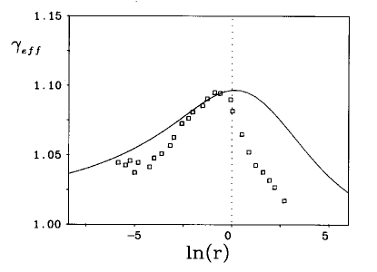
Figure 1: Effective exponent of the susceptibility for $g=1.0$ and $u=u_{{}_{I}}$ versus $\ln(r)$. The momentum scale is chosen as $\mu=1$. Experimental data on $LiTbF_{4}$ from Ref.[20].

3.2 Crossover from isotropic to directed percolation

Another example, where the presence of a second length scale leads to a crossover in the critical behavior, is the physics of biased percolation. The patterns generated by these percolation models incorporate self-similar as well as self-affine clusters.

In ordinary percolation, sites or bonds are filled at random with probability $p$ [22]. The percolation process then proceeds along paths connecting occupied nearest neighbors. The clusters formed by nearest-neighbor links are self-similar, i.e., they display isotropic scaling. In directed percolation [23] the links between nearest neighbors have a bias in one preferred direction $t$, such that the percolation process advances along this direction only. The size of the clusters in the preferred direction is characterized by a length scale different from that in the perpendicular direction. If percolation in the positive $t$ direction is merely favored with a certain probability with respect to the negative $t$ direction, but propagation “backward” in time is still admitted, the situation will be more complicated. If the “anisotropy” $g$ is low, one expects almost isotropic scaling behavior in a large region of the phase diagram. However, when the critical region near the percolation threshold $p_{c}$ is approached, self-affine scaling will become apparent.

In order to give a quantitative description of the crossover from isotropic to directed percolation we investigate the pair correlation function $G({\bf r}_{2},{\bf r}_{1})$, which measures the probability that sites ${\bf r}_{2}=({\bf x}_{2},t_{2})$ and ${\bf r}_{1}=({\bf x}_{1},t_{1})$ belong to the same cluster. Following the work of Cardy and Sugar [12], and Benzoni and Cardy [13], the pair correlation function (the superscript “0” denotes unrenormalized quantities) is found to be a sum $G^{0}({\bf r}_{2};{\bf r}_{1})=\sum_{m,n=1}^{\infty}[(-i)^{m+n-2}/m!n!]G^{0}_{mn}({\bf r}_{2};{\bf r}_{1})$, where the correlation functions $G^{0}_{mn}$ are obtained from the effective action

$${\cal J}=\!\int\!\! d^{D}x\!\!\int\!\!dt\biggl{\{}{\tilde{\phi}}_{0}({\bf x},t)\!\left[r_{0}-{\bf\nabla}^{2}-{1\over c_{0}^{2}}\partial_{t}^{2}+{2g_{0}\over c_{0}}\partial_{t}\right]\!\phi_{0}({\bf x},t)$$ (22)

$$+{u_{0}\over 2}\left[{\tilde{\phi}}_{0}({\bf x},t)^{2}\phi_{0}({\bf x},t)-{\tilde{\phi}}_{0}({\bf x},t)\phi_{0}({\bf x},t)^{2}\right]\biggr{\}}\,,$$

with $r_{0}\propto p-p_{c}$. The effective action is renormalized upon introducing renormalized fields $\phi=Z_{\phi}^{1/2}\phi_{0}$ and ${\tilde{\phi}}=Z_{\phi}^{1/2}{\tilde{\phi}}_{0}$, dimensionless renormalized parameters $r=Z_{\phi}^{-1}Z_{r}(r_{0}-r_{0c})\mu^{-2}$, $c^{2}=Z_{\phi}Z_{c}^{-1}c_{0}^{2}$, $g=Z_{\phi}^{-1/2}Z_{c}^{-1/2}Z_{g}g_{0}\mu^{-1}$, and a renormalized coupling constant $u=Z_{\phi}^{-3/2}Z_{u}u_{0}B_{d}^{1/2}\mu^{(d-6)/2}$. $B_{d}=\Gamma(4-d/2)/(4\pi)^{d/2}$ is a geometric factor, and $r_{0c}$ denotes the fluctuation-induced shift of the percolation threshold. The five independent multiplicative renormalization constants are then uniquely determined by extracting the ultraviolet singularities of the two- and three-point vertex functions at finite mass $r_{0}=\mu^{2}$. In the course of renormalizing the model it is convenient to introduce an effective anharmonic coupling $v=u^{2}cI^{d}_{17}(g)$.

From an analysis of the renormalization group equation (where for notational convenience we have taken $\mu=1$ in the following)

$$\Gamma_{11}(\{x\},{\bf q},\omega)=\ell^{2}e^{\int_{1}^{\ell}\zeta_{\phi}(\ell^{\prime})d\ell^{\prime}/\ell^{\prime}}{\hat{\Gamma}}_{11}\left(r(\ell),v(\ell),{{\bf q}\over\ell},{g(\ell)\omega\over c(\ell)\ell},{\omega^{2}\over c(\ell)^{2}\mu^{2}\ell^{2}}\right)\,.$$ (23)

one finds four independent critical exponents. At a fixed point $v^{*}$ using the matching condition ${\ell=q}$, one arrives at the following general self-affine scaling form

$$\Gamma_{11}(r,c,g,u,{\bf q},\omega)\propto q^{2-\eta_{\perp}}{\hat{\Gamma}}_{11}\left({r\over q^{1/\nu_{\perp}}},v^{*},1,{g\omega/c\over q^{z}},{\omega^{2}/c^{2}\over q^{2z(1-\Delta)}}\right)\,,$$ (24)

with the critical exponents $\eta_{\perp}=-\zeta_{\phi}^{*}$, $\nu_{\perp}=-1/\zeta_{r}^{*}$, $z=1+\zeta_{c}^{*}-\zeta_{g}^{*}$, and $z\Delta=-\zeta_{g}^{*}$. Here, $\eta_{\perp}$ and $\nu_{\perp}$ correspond to the two independent indices familiar from the theory of static critical phenomena. The exponent $z$ was introduced in analogy to a dynamical critical exponent, and in our case is related to the anisotropic scaling behavior. Finally, $\Delta$ is a positive crossover exponent describing the transition from isotropic to directed percolation. It stems from the fact that there appear two different scaling variables for the “frequency” $\omega$ in Eq. (24). In the asymptotic limit of directed percolation, $g\rightarrow\infty$, the second scaling variable disappears, and the scaling behavior is described by the three exponents $\eta_{\perp}$, $\nu_{\perp}$, and $z$.

Similarly, with the choices $\ell=\left(g\omega/c\right)^{1/(1+\zeta_{c}^{*}-\zeta_{g}^{*})}$ and $\ell=r^{-1/\zeta_{r}^{*}}$ the longitudinal exponents $2-\eta_{\parallel}=(2-\eta_{\perp})/z$ and $\nu_{\parallel}=z\nu_{\perp}$ and the (“susceptibility”) exponent $\gamma=\nu_{\perp}(2-\eta_{\perp})=\nu_{\parallel}(2-\eta_{\parallel})$, respectively. In the special case of isotropic percolation ($g_{0}=0$), the scaling relations simplify considerably, describing self-similar scaling with only two independent critical exponents $\eta=-\zeta_{\phi}^{*}$ and $\nu=-1/\zeta_{r}^{*}$.

We have seen that both the self-similar and the self-affine scaling behavior are within the scope of the present theory, at least for dimensions $d<5$; for $5<d\leq 6$ the model is not renormalizable in the directed limit, and simply characterized by the exponents corresponding to the Gaussian fixed point $v^{*}_{\rm GD}$, with logarithmic corrections for $d=5$. This again emphasizes the fact that no expansion with respect to a fixed upper critical dimension can be applied consistently. In order to study the entire crossover region between these asymptotic regimes, the coupled set of flow equations have to be solved numerically. Fig. 2 shows the flow diagram (at $d=3$ dimensions) for the effective couplings $v(\ell)$ and ${\bar{g}}(\ell)$, whose topology is determined by the four fixed points. The separatrix connecting $v^{*}_{\rm I}$ with the infrared-stable fixed point $v^{*}_{\rm D}$ describes the universal crossover features from isotropic to directed percolation.

Figure 2: Renormalization-group trajectories in the $(v,{\tilde{g}})$ parameter space for the crossover from isotropic to directed percolation (to one-loop order) in $d=3$ dimensions.

The interchange from self-similar to self-affine scaling is most conveniently described by introducing effective exponents for the pair-correlation function. Using the zero-loop result for the two-point vertex function

$$\Gamma_{11}(\{x\},{\bf q},\omega)=\ell^{2}e^{\int_{1}^{\ell}\zeta_{\phi}(\ell^{\prime})d\ell^{\prime}/\ell^{\prime}}\left[r(\ell)+\left({q\over\ell}\right)^{2}+{\omega^{2}\over\ell^{2}c(\ell)^{2}}+2i{\omega g(\ell)\over\ell c(\ell)}\right]\,,$$ (25)

we specialize to $r=0$ and ${\bf q}={\bf 0}$ and define

$$2-\eta_{\parallel\,\rm eff}(\omega)={d\ln{\sqrt{\mid\Gamma_{11}(0,{\bf 0},\omega)\mid^{2}}}\over d\ln\omega}\quad.$$ (26)

Using $\left|\omega^{2}/\ell^{2}c(\ell)^{2}+2i\omega g(\ell)/\ell c(\ell)\right|^{2}=1$ yields $2-\eta_{\parallel\,\rm eff}(\ell)=[2+\zeta_{\phi}(\ell)]d\ln\ell/d\ln\omega$. Similarly, in the case $r=\omega=0$ one finds

$$2-\eta_{\perp\,{\rm eff}}(q)={d\ln\Gamma_{11}(0,{\bf q},0)\over d\ln q}\,,$$ (27)

which reduces to $2-\eta_{\perp\,{\rm eff}}=2+\zeta_{\phi}(\ell)$, if $(q/\ell)^{2}=1$ is inserted. Finally, considering ${\bf q}={\bf 0}$ and $\omega=0$ one introduces

$$\gamma_{\rm eff}(r)={d\ln\Gamma_{11}(r,0,0)\over d\ln r}\quad,$$ (28)

and choosing the matching condition $r(\ell)=1$ we find $\gamma_{\rm eff}(\ell)=-[2+\zeta_{\phi}(\ell)]/\zeta_{r}(\ell)$.

The flow of the effective exponents $\eta_{\parallel\,\rm eff}(\ell)$, $\eta_{\perp\,\rm eff}(\ell)$, and $\gamma_{\rm eff}(\ell)$ in $d=3$ dimensions is depicted in Fig. 3, with the initial value for the coupling $v(1)=v^{*}_{\rm I}$ of the isotropic scaling fixed point. The dependence on the anisotropy scale $g$ was eliminated by plotting versus the scaling variable $\ln g(\ell)$; the graphs corresponding to different initial values $g(1)$ then all collapse onto one master curve. The most important conclusion to be drawn from Fig. 3 is that the anisotropy scale, at which the crossover occurs, considerably differs for the effective exponents defined above. $\eta_{\parallel\,\rm eff}$ starts to cross over from the isotropic to the directed fixed point value already at $\ln g(\ell_{\rm cross})\approx-0.8$, whereas $\gamma_{\rm eff}$ shows this crossover at $\ln g(\ell_{\rm cross})\approx-0.2$, and $\eta_{\perp\,\rm eff}$ only at $\ln g(\ell_{\rm cross})\approx+0.8$. Note that the sizeable change of $\eta_{\parallel\,\rm eff}$ is already apparent at mean-field level, where it acquires the values $0$ and $1$ in the isotropic and directed limit, respectively. However, a crossover of the exponents $\eta_{\perp\,\rm eff}$ and $\gamma_{\rm eff}$ requires the $\zeta$ functions at least on the one-loop level.

Figure 3: Effective exponents $\eta_{\parallel\,{\rm eff}}(\ell)$ (solid), $\eta_{\perp\,{\rm eff}}(\ell)$ (dashed), and $\gamma_{\rm eff}(\ell)$ (dotted) for the connectivity as functions of the running anisotropy parameter $g(\ell)$ for a fixed initial value of the coupling constant $v(1)=v^{*}_{\rm I}$.

3.3 Multicritical behavior in lattice boson models

The critical behavior at the zero temperature Mott insulator to superfluid (S-I) transition of lattice boson models can be analyzed in terms of the effective action [14]

$${\cal S}={\textstyle\frac{1}{2}}\int_{{\bf k},\omega}\left[r_{0}+k^{2}+\omega^{2}+2ig_{0}\omega\right]\mid\phi_{0}({\bf k},\omega)\mid^{2}+{u_{0}\over 4}\int_{{\bf x},t}\mid\phi_{0}({\bf x},t)\mid^{4}\,,$$ (29)

where the field $\phi$ serves as the order parameter for superfluidity. The parameters $r_{0}$ and $u_{0}$ can be calculated from the underlying microscopic lattice models. One finds that $g_{0}(\mu,J)=\partial r_{0}(\mu,J)/\partial\mu$, where $\mu$ and $J$ are the chemical potential and the hopping matrix element of the lattice model, respectively. Since in mean field theory the phase boundary is given by $r_{0}(\mu,J)=0$, the point $g_{0}=0$ constitutes a multicritical point for S-I transition.

Before starting the renormalization group calculation of the crossover scaling functions, we give a brief review of the phenomenological scaling theory [14].The quantum phase transition at $T=0$ is characterized by both a diverging length scale $\xi\propto r^{-\nu}$ and a diverging time scale $\Omega^{-1}\propto r^{-\nu z}$. Near the multicritical point $(r,g)=(0,0)$ the singular part of the free energy shows crossover scaling behavior

$$f_{s}\propto r^{(d+z)\nu}{\tilde{f}}_{s}(g/r^{\phi})\,,$$ (30)

with $\phi$ being the crossover scaling exponent. As discussed in section 2 the crossover scaling function ${\tilde{f}}_{s}(x)$ has to become singular at some critical value $x_{c}$ in order to describe the crossover from primary to secondary critical exponents.

Here we use the field theoretic method described in section 2 to determine the effective exponents. We introduce renormalization factors by $\phi=Z_{\phi}^{1/2}\phi_{0}$, and dimensionless renormalized parameters $r=Z_{\phi}^{-1}Z_{r}(r_{0}-r_{0c})\mu^{-2}$, $g=Z_{\phi}^{-1/2}Z_{g}g_{0}\mu^{-1}$, and a renormalized coupling constant $u=Z_{\phi}^{-2}Z_{u}u_{0}B_{d}\mu^{d-3}$. The crossover induced by the term linear in the frequency $\omega$ leads to a reduction of the upper critical dimension from $d_{c}=3$ to $d_{c}=2$. From a one-loop calculation we find [24] for the renormalization factors $Z_{\phi}=1$, $Z_{g}=1$, and

$$Z_{r} =1-{u\over\varepsilon}\int_{o}^{1}dxx^{m/2-1}(x+g^{2})^{(d-m-n)/2}\,,$$ (31)

$$Z_{u} =1-{1\over\varepsilon}{\bar{A}}u-{1\over\varepsilon}{\bar{B}}u\,,$$ (32)

where ${\bar{A}}={\textstyle\frac{1}{4}}I_{12}^{d}(g)$ and ${\bar{B}}=(1+g^{2})^{\varepsilon/2}$ with $\varepsilon=3-d$ being the distance to the upper critical dimension of the primary fixed point. One should note that $Z_{g}=1$ is valid to all orders in perturbation theory since there is no singular contribution proportional to $\omega$. The one-loop theory may be further improved by taking into account results which become exact in the limit $g\rightarrow\infty$. In this limit the special (“causal”) structure of the propagator implies that the corrections to the bare two-point vertex function vanish to all orders in perturbation theory [25, 14], i.e., $Z_{r}(g\rightarrow\infty)=1$ exactly. Furthermore, there are only “ladder”-diagrams [25] contributing to the renormalization of $u$, which form a geometric series with the result

$$u\mu^{\varepsilon}={u_{0}\over 1+Au_{0}}\,,$$ (33)

with $A={1\over\varepsilon}B_{d}\mu^{-\varepsilon}{\bar{A}}$. Now, in order to improve the one-loop result we suggest to resum the ladder diagrams corresponding to the one-loop term $Au_{0}$, while still using the one-loop result for all the other terms. This procedure amounts to

$$u\mu^{\varepsilon}={u_{0}\over 1+Au_{0}}-Bu_{0}\,,$$ (34)

where $B={1\over\varepsilon}B_{d}\mu^{-\varepsilon}{\bar{B}}$. Equivalently to one loop order we could also use $u\mu^{\varepsilon}=u_{0}/(1+(A+B)u_{0})$.

Upon defining Wilson’s flow functions as in section 3.2 one can study the behavior of the vertex function $\Gamma_{11}$ under renormalization group transformations

$$\Gamma_{11}(\mu,r,g,u;q,\omega)=\mu^{2}\ell^{2}{\hat{\Gamma}}_{11}\left(r(\ell),g(\ell),v(\ell);{q\over\mu\ell},{\omega\over\mu\ell}\right)\,,$$ (35)

where it is convenient to introduce the effective coupling constant $v=uI_{12}^{d}(g)$. At the secondary fixed point $v^{*}$ one finds using the matching condition $r(\ell)=1$

$$\Gamma_{11}(\mu,r,g,u;q,\omega)\propto\ell^{2\nu}{\hat{\Gamma}}_{11}(1,g\xi,v^{*};q\xi,\omega\xi)\,,$$ (36)

where $\xi\propto r^{-\nu}$. Since $Z_{g}=1$ to all orders in perturbation theory, one finds that the crossover exponent $\phi$ is exactly given by the correlation length exponent. One can define an effective exponent $\nu(\ell)=-1/\zeta_{r}(\ell)$, the flow of which is obtained from a solution of the flow equations [24]. An effective dynamic exponent may be obtained by analyzing the pole $\Gamma$ of the dynamic susceptibility (we have used the 0–loop result for the scaling function)

$$\Gamma\propto\mu\ell\left[g(\ell)-\sqrt{r(\ell)+g^{2}(\ell)+q^{2}/(\mu\ell)^{2}}\right]\,,$$ (37)

the scaling behavior of which may be analyzed in various ways [24]. At the critical point $r=0$ with $q/\mu\ell=1$ we get

$$\Gamma\propto q\left[g/q-\sqrt{1+g^{2}/q^{2}}\right]$$ (38)

describing the trivial crossover from $z=1$ to $z=2$ as $q\rightarrow 0$. Note, that there is, however, nontrivial crossover behavior for the exponent of the correlation length from the Ising fixed point value $\nu^{*}_{I}$ to the Gaussian fixed point value $1/2$.

4 Summary and outlook

In this paper a field theoretic renormalization group technique using normalization conditions was presented, which allows for the description of crossover phenomena, where the primary and secondary fixed point have different upper critical dimension. This method can be thought of as the field theoretic version of Nelson’s trajectory integral method. It has the advantage of being capable of describing quite complicated crossover scenarios. Especially, using the field theoretic renormalization method one can derive an explicit expression for the crossover scaling function, where the regular and singular parts are already separated.

We have employed this method for three particular interesting crossover phenomena from various fields of critical phenomena, namely magnetic phase transitions with dipolar anisotropy, biased percolation problems, and the multicritical point of the Mott insulator to superfluid transition in Bose lattice models.

Another variant of Amit and Goldschmidt’s generalized minimal subtraction procedure has been used by Stephens and O’Connor [26, 27] to investigate crossover phenomena ranging from finite size scaling problems to quantum-classical crossover.

We close with emphasizing that the method could be applied to various other quite interesting crossover phenomena. Since it is quite likely that many experiments are not done in the asymptotic but in the crossover regime, it seems highly desirable to perform such calculations in order to get a quantitative understanding of the critical behavior.

References

- [1] For a recent review on phase transitions and critical phenomena see e.g. F. Schwabl and U.C. Täuber, in Encyclopedia of Applied Physics, Vol. 13 (VCH Publishers, 1995) 343.
- [2] E. Riedel and F. Wegner, Z. Phys. 255 (1969) 195; Phys. Rev. Lett. 24 (1970) 730; 24 (1970) 930(E).
- [3] P. Pfeuty, D. Jasnow, and M.E. Fisher, Phys. Rev. B 10 (1974) 251.
- [4] D.R. Nelson, Phys. Rev. B 11 (1975) 3504.
- [5] D.J. Amit and Y.Y. Goldschmidt, Ann. of Phys. 114 (1978) 356.
- [6] D. J. Amit, Field Theory, the Renormalization Group, and Critical Phenomena, 2nd ed. (World Scientific, Singapore, 1984).
- [7] I. D. Lawrie, J. Phys. A 14 (1981) 2489; ibid. 18 (1985) 1141.
- [8] E. Frey and F. Schwabl, J. Phys. (Paris) Colloq. 48 (1988) C8-1569; Phys. Rev. B 43 (1991) 833.
- [9] E. Frey and F. Schwabl, Phys. Rev. B 42 (1990) 8261.
- [10] E. Frey, U.C. Täuber, and F. Schwabl, Europhys. Lett. 26 (1994) 413; Phys. Rev. B 49 (1994) 5058.
- [11] U. C. Täuber and F. Schwabl, Phys. Rev. B 46 (1992) 3337; ibid 48 (1993) 186.
- [12] J. L. Cardy and R. L. Sugar, J. Phys. A 13 (1980) L423.
- [13] J. Benzoni and J. L. Cardy, J. Phys. A 17 (1984) 179.
- [14] M.P.A. Fisher, P.B. Weichman, G. Grinstein, and D.S. Fisher Phys. Rev. B 40 (1989) 546.
- [15] R. Schloms and V. Dohm, Nucl. Phys. B 328 (1989) 639; Phys. Rev. B 42 (1990) 6142.
- [16] A.I. Larkin and D.E. Khmelnitskii, Sov. Phys. JETP 29 (1969) 1123.
- [17] A. Aharony, Phys. Rev. B 8 (1973) 3363; Phys. Lett. 44A (1973) 313.
- [18] E. Brezin and J. Zinn-Justin, Phys. Rev. B 13 (1976) 251.
- [19] G. Ahlers, A. Kornblit and H.J. Guggenheim, Phys. Rev. Lett. 34 (1975) 1227.
- [20] R. Frowein, J. Kötzler, B. Schaub and H.G. Schuster, Phys. Rev. B 25 (1982) 4905.
- [21] T. Nattermann and J. Trimper, J Phys. C 9 (1976) 2589.
- [22] For a review on the theory of percolation, see e.g. D. Stauffer and A. Aharony, Introduction to Percolation Theory, 2nd ed. (Taylor and Francis, London, 1992).
- [23] For a review, see W. Kinzel, in: Percolation Structures and Processes, Ann. Isr. Phys. Soc. Vol. 5, Eds. G. Deutscher, R. Zallen, and J. Adler (Bar-Ilan University, 1983), p. 425.
- [24] E. Frey, (1995) unpublished.
- [25] D.I. Uzunov, Phys. Lett. 87A 11 (1981).
- [26] D. O’Connor and C.R. Stephens, Nucl. Phys. B 360 (1991) 297; J. Magn. Magn. Mat. 104-107 (1992) 297; J. Phys. A 25 (1992) 101; Phys. Rev. Lett. 72 (1993) 506; Int. J. of Mod. Phys. 9 (1994) 2805.
- [27] F. Freire, D. O’Connor, and C.R. Stephens, J. Stat. Phys. 74 (1994) 219.