Theory of Chiral Order in Random Copolymers

Abstract

Recent experiments have found that polyisocyanates composed of a mixture of opposite enantiomers follow a chiral “majority rule:” the chiral order of the copolymer, measured by optical activity, is dominated by whichever enantiomer is in the majority. We explain this majority rule theoretically by mapping the random copolymer onto the random-field Ising model. Using this model, we predict the chiral order as a function of enantiomer concentration, in quantitative agreement with the experiments, and show how the sharpness of the majority-rule curve can be controlled.

Cooperative chiral order plays a vital role in the self-assembly of ordered supramolecular structures in liquid crystals [1], organic thin films [2, 3, 4, 5], and lipid membranes [6, 7, 8, 9, 10, 11, 12]. One particularly simple and well-controlled example of cooperative chiral order is in random copolymers. Recent experiments have found that polyisocyanates formed from a mixture of opposite enantiomers follow a chiral “majority rule” [13]. The chiral order of the copolymer, measured by optical activity, responds sharply to slight differences in the concentrations of the enantiomers, and is dominated by whichever enantiomer is in the majority. In this paper, we show that the majority rule can be understood through a mapping of the random copolymer onto the random-field Ising model [14, 15, 16]. Using this model, we predict the chiral order as a function of enantiomer concentration, in quantitative agreement with the experiments, and show that the sharpness of the majority-rule curve is determined by two energy scales associated with the chiral packing of monomers.

In a series of experiments, Green et al. have investigated chiral order in polyisocyanates [17]. This polymer consists of a carbon-nitrogen backbone with a pendant group attached to each monomer, as shown in Fig. 1. Although the backbone is nonchiral, steric constraints force the molecule to polymerize in a helical structure. If the pendant group is also nonchiral, the helix is randomly right- or left-handed. A long chain then consists of domains of fixed helicity, separated by occasional helix reversals. On average, there are equal right- and left-handed domains, leading to zero net optical activity. However, if the pendant group is chiral, there is a preference for one sense of the helix, which leads to a net optical activity. Because of the cooperative interaction between the monomers in a domain, even a very small chiral influence leads to a large optical activity [18]. Most recently, Green et al. have synthesized random copolymers with a mixture of right- and left-handed enantiomeric pendant groups, with concentrations $p$ and $1-p$, respectively [13]. The resulting optical activity, shown in Fig. 2, has a surprisingly sharp dependence on $p$. A 56/44 mixture of enantiomers has almost the same optical activity as a pure 100/0 homopolymer, and even a 51/49 mixture has a third of that optical activity.

To explain this cooperative chiral order theoretically, we map the random copolymer onto the one-dimensional random-field Ising model, a standard model in the theory of random magnetic systems [14, 15, 16]. Although related models have been applied to other polymer systems [19, 20, 21, 22], our theory gives a new, direct correspondence between the Ising order parameter and the optical activity. This correspondence provides a novel experimental test of predictions for the random-field Ising model. Let the Ising spin $\sigma_{i}=\pm 1$ represent the sense of the polymer helix at the monomer $i$. The energy of a polymer can then be written as

$$H=-J\sum_{i=1}^{N-1}\sigma_{i}\sigma_{i+1}-\sum_{i=1}^{N}h_{i}\sigma_{i}.$$ (1)

Here, the random field $h_{i}$ specifies the enantiomeric identity of the pendant group on monomer $i$: $h_{i}=+h$ if it is right-handed (with probability $p$) and $h_{i}=-h$ if it is left-handed (with probability $1-p$). This field is a quenched random variable; it is fixed by the polymerization of each individual chain. The parameter $2h$ is the energy cost of a right-handed monomer in a left-handed helix, or vice versa. Molecular modeling gives $2h\approx 1.7$ kJ/mol (0.4 kcal/mol) for the pendant group used in these experiments[23]. The parameter $2J$ is the energy cost of a helix reversal. Fits of the optical activity of pure homopolymers as a function of temperature $T$ give $2J\approx 17$ kJ/mol (4 kcal/mol) [18]. Note that $2J$ is much greater than $k_{B}T\approx 2.5$ kJ/mol (0.6 kcal/mol), but $2h<k_{B}T$. The degree of polymerization $N$ ranges from 350 to 5800 in the experiments [13]. The magnetization of the Ising model,

$$M=\left\langle\frac{1}{N}\sum_{i=1}^{N}\sigma_{i}\right\rangle,$$ (2)

corresponds to the chiral order parameter that is measured by optical activity. To predict the optical activity of the random copolymer as a function of enantiomer concentration, we must calculate $M$ as a function of $p$.

To calculate the order parameter $M$, we note that each chain consists of domains of uniform helicity $\sigma_{i}$. As an approximation, suppose that each domain has length $L$, which is to be determined. Each domain responds to the total chiral field $h_{\rm tot}=\sum h_{i}$ of the monomers in it. Because the domain is uniform, the response is $M(h_{\rm tot})=\tanh(h_{\rm tot}/k_{B}T)$, equivalent to a single spin in a magnetic field. Averaging over the probability distribution $P(h_{\rm tot})$, we obtain

$$M=\int_{-\infty}^{\infty}dh_{\rm tot}P(h_{\rm tot})\tanh\left(\frac{h_{\rm tot}}{k_{B}T}\right).$$ (3)

The probability distribution $P(h_{\rm tot})$ is a binomial distribution. For large domains, it can be approximated by a Gaussian with mean ${2hL(p-\frac{1}{2})}$ and standard deviation ${2h[Lp(1-p)]^{1/2}}$. For $p\approx\frac{1}{2}$, the standard deviation becomes $hL^{1/2}$. Furthermore, if the width of the Gaussian is much greater than the width of the tanh, $hL^{1/2}\gg k_{B}T$, then the tanh can be approximated by a step function. The expression for $M$ then becomes

$$M\approx{\rm erf}\left[\left(2L\right)^{1/2}\left(p-\frac{1}{2}\right)\right].$$ (4)

We must now estimate the domain size $L$. The domain size is determined by (a) the distance $L_{\rm rf}$ between helix reversals that are induced by the random field, (b) the distance $L_{\rm th}$ between helix reversals that are induced by thermal fluctuations, and (c) the chain length $N$. Because each of these effects contributes to the density $1/L$ of domain boundaries, we expect

$$\frac{1}{L}\approx\frac{1}{L_{\rm rf}}+\frac{1}{L_{\rm th}}+\frac{1}{N}.$$ (5)

For $p\approx\frac{1}{2}$, the random-field domain size $L_{\rm rf}$ can be estimated using a variation of the Imry-Ma argument for the random-field Ising model [14]. A domain forms when the field energy $hL^{1/2}$ grows to equal the boundary energy $J$. By equating these two energies, we obtain the random-field domain size

$$L_{\rm rf}\approx\left(\frac{J}{h}\right)^{2}.$$ (6)

With the values $2J\approx 17$ kJ/mol (4 kcal/mol) and $2h\approx 1.7$ kJ/mol (0.4 kcal/mol) appropriate for the experimental system, the random-field domain size becomes $L_{\rm rf}\approx 100$ monomers. By comparison, the thermal domain size is $L_{\rm th}=e^{2J/k_{B}T}\approx 800$, and the chain length is $N\approx 350$–$5800$. Because $L_{\rm rf}$ is much less than $L_{\rm th}$ and $N$, we obtain $L\approx L_{\rm rf}$; i. e., the domain size is limited by random-field effects.

To test this approximate calculation explicitly, and to obtain a more precise value of the domain size, we performed numerical simulations of the random-field Ising model. In these simulations, we used a series of chain lengths from 4 to 230, and used the values of $J$ and $h$ appropriate for the experiments. For each chain length, we constructed an explicit realization of the random field, then calculated the partition function and order parameter using transfer-matrix techniques. We then averaged the order parameter over at least 1000 realizations of the random field. Figure 3 shows $M$ as a function of $p$ for chain length $N=230$. These results can be fit very well to Eq. (4), with the domain size $L(230)=96$. The results for other values of $N$ can be fit equally well. Figure 4 shows the fitted domain size $L(N)$ as a function of chain length $N$. These results can be extrapolated using $1/L(N)=1/L_{\rm max}+1/N$, with $L_{\rm max}=164$. This random-field domain size agrees well with Eq. (6), especially considering that the Imry-Ma argument is only a scaling argument. Thus, the chiral order parameter should indeed be given by Eq. (4), with the extrapolated domain size $L=164$.

To compare our theory with the experiment, we plot our prediction for the chiral order parameter $M$ on top of the experimental data for the optical activity in Fig. 2. The prediction agrees very well with the data. In particular, $M$ saturates at $(p-\frac{1}{2})\approx 0.06$, a 56/44 composition, in agreement with the data. This saturation point is a direct measure of $1/(2L)^{1/2}$, which is controlled by the ratio of the two energy scales $J$ and $h$. We emphasize that the theory matches the experimental data with no adjustable parameters, other than the relative scale of the optical-activity axis and the order-parameter axis. That relative scale is the optical activity of a pure 100/0 homopolymer.

We can make two remarks about these results. First, both the random-field domain size $L_{\rm rf}$ and the thermal domain size $L_{\rm th}$ depend on $p$. The Imry-Ma argument above applies only to the regime where $p\approx\frac{1}{2}$. This is the appropriate regime for understanding the experiments, because all the significant variation in the chiral order parameter $M$ occurs around $p\approx\frac{1}{2}$. Outside that regime, $M$ saturates at $\pm 1$, and it is not sensitive to $L$. Second, the fact that $L_{\rm rf}\ll L_{\rm th}$ shows that quenched disorder is much more significant than thermal disorder in this copolymer system. Thus, the system is effectively in the low-temperature limit. If the temperature $T$ were increased so that $L_{\rm th}\lesssim L_{\rm rf}$, then thermal disorder (i. e. entropy) would become more significant. However, that would require a temperature of $T\gtrsim 400$ K, which is unrealistic because the system would degrade chemically.

Using our theory, we can make two predictions for future experiments. First, the experiment could be repeated using different degrees of polymerization. For short chains, the domain size $L$ is limited by the chain length $N$, particularly for $N\lesssim 200$, as shown in Fig. 4. Thus, shorter chains should give a broader version of the majority-rule curve. By contrast, longer chains should not give a sharper majority-rule curve, because the chains are already in the regime where $L$ is approximately independent of $N$. Second, the experiment could be repeated using pendant groups that are “less chiral,” i. e. polyisocyanates with a lower energy cost for a right-handed monomer in a left-handed helix. A lower value of the chiral field $h$ should give a larger value of the domain size $L\approx(J/h)^{2}$, and hence a sharper majority-rule curve. (This prediction applies as long as $L_{\rm rf}\ll L_{\rm th}$, or $2h\gg 2Je^{-J/k_{B}T}\approx 0.6$ kJ/mol [0.14 kcal/mol]. Thus, $h$ can be reduced by a factor of 3 from its value in the current experiments, and the majority-rule curve can become 3 times sharper. Beyond that point, the sharpness will be limited by the thermal domain size.) This second prediction might seem counter-intuitive, because one might expect a smaller chiral field to give a smaller effect. However, this prediction is reasonable, considering that the majority-rule curve is limited by the number of monomers that cooperate inside a single domain. If the local chiral field is reduced, then each monomer is more likely to have the same helicity as its neighbors, independent of the local chiral field, and hence the cooperativity increases.

Finally, we note that the sharp majority-rule curve in polyisocyanates can be exploited in an optical switch [24]. If a mixture of enantiomers is exposed to a pulse of circularly polarized light, one enantiomer is preferentially excited into a higher-energy state. That state can decay into either chiral form. Thus, a light pulse depletes the preferentially excited enantiomer and changes the enantiomer concentration $p$, which changes the optical activity. In other systems, this approach has been limited by the fact that light pulses induce only a slight change in $p$, and hence only a slight change in optical activity. However, in polyisocyanates, a slight change in $p$ close to $p=\frac{1}{2}$ is sufficient to induce a very significant change in optical activity. Indeed, this polymer has almost a binary response to changes in $p$, which is needed for an optical switch. Our theory shows how to optimize the majority-rule curve for use in an optical switch.

In conclusion, we have shown that the cooperative chiral order in polyisocyanates can be understood through the random-field Ising model. The energy scales $J$ and $h$, which arise from the chiral packing of the monomers, give the random-field domain size $L_{\rm rf}$, which indicates how many monomers are correlated in a single domain. This domain size determines the sharpness of the majority-rule curve. Our theory agrees well with the current experiments, and it shows how future experiments can control the chiral order.

We thank M. M. Green and J. M. Schnur for many helpful discussions.

FIG. 1.: Molecular structure of the polyisocyanate with enantiomeric pendant groups derived from citronellic acid, which was studied in Ref. [13].

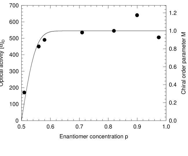
FIG. 2.: Symbols: Optical activity $[\alpha]_{D}$ of the random copolymer at the sodium D-line as a function of enantiomer concentration $p$, from Ref. [13]. Solid line: Theoretical prediction for the chiral order parameter $M$ from Eq. (4), with the domain size $L=164$. The prediction agrees with the data with no adjustable parameters, other than the relative scale of the vertical axes.

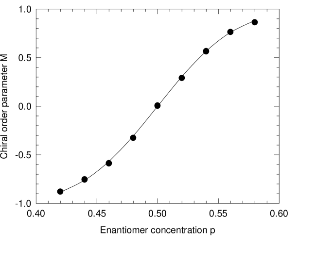
FIG. 3.: Numerical simulation of the chiral order parameter $M$ as a function of enantiomer concentration $p$ for chain length $N=230$. The solid line shows a fit to the prediction of Eq. (4), which gives the domain size $L(230)=96$.

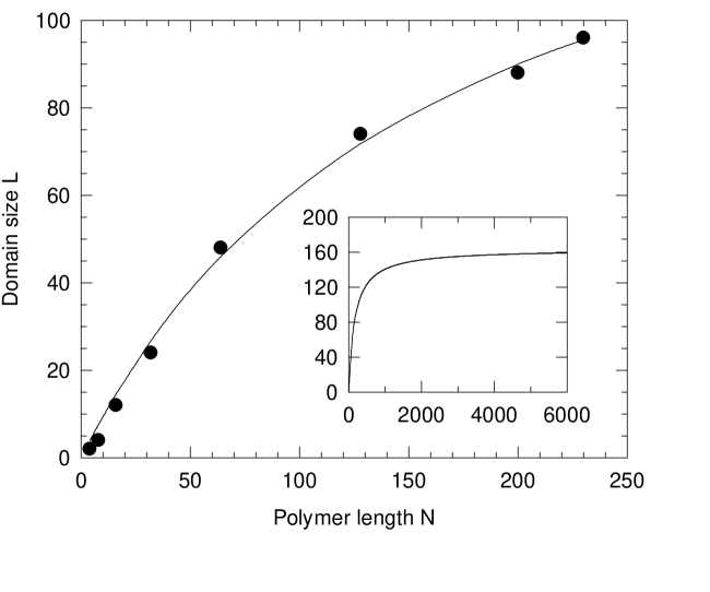
FIG. 4.: The domain size $L(N)$ from numerical simulations for several values of the chain length $N$. The solid line shows a fit to the extrapolation form $1/L(N)=1/L_{\rm max}+1/N$, or $L(N)=L_{\rm max}N/(L_{\rm max}+N)$, which gives $L_{\rm max}=164$. The inset shows the extrapolation up to $N=6000$.

REFERENCES

- [1] P.-G. de Gennes and J. Prost, The Physics of Liquid Crystals (Clarendon, Oxford, second edition, 1993).
- [2] J. V. Selinger, Z.-G. Wang, R. F. Bruinsma, and C. M. Knobler, Phys. Rev. Lett. 70, 1139 (1993).
- [3] C. J. Eckhardt et al., Nature 362, 614 (1993).
- [4] R. Viswanathan, J. A. Zasadzinski, and D. K. Schwartz, Nature 368, 440 (1994).
- [5] J. V. Selinger and R. L. B. Selinger, Phys. Rev. E 51, R860 (1995).
- [6] J. M. Schnur, Science 262, 1669 (1993).
- [7] W. Helfrich and J. Prost, Phys. Rev. A 38, 3065 (1988).
- [8] P. Nelson and T. Powers, J. Phys. II France 3, 1535 (1993).
- [9] D. S. Chung, G. B. Benedek, F. M. Konikoff, and J. M. Donovan, Proc. Natl. Acad. Sci. USA 90, 11341 (1993).
- [10] J. V. Selinger and J. M. Schnur, Phys. Rev. Lett. 71, 4091 (1993).
- [11] J. M. Schnur et al., Science 264, 945 (1994).
- [12] C.-M. Chen, T. C. Lubensky, and F. C. MacKintosh, Phys. Rev. E 51, 504 (1995).
- [13] M. M. Green et al., J. Am. Chem. Soc. 117, 4181 (1995).
- [14] Y. Imry and S.-K. Ma, Phys. Rev. Lett. 35, 1399 (1975).
- [15] T. Nattermann and J. Villain, Phase Transitions 11, 5 (1988).
- [16] T. Nattermann and P. Rujan, Int. J. Mod. Phys. B 3, 1597 (1989).
- [17] M. M. Green et al., Science 268, 1860 (1995).
- [18] S. Lifson, C. Andreola, N. C. Peterson, and M. M. Green, J. Am. Chem. Soc. 111, 8850 (1989).
- [19] A. L. Kholodenko and K. F. Freed, Macromolecules 15, 899 (1982).
- [20] J.-C. Lin, P. L. Taylor, and R. Rangel, Phys. Rev. E 47, 981 (1993).
- [21] R. Zhang and P. L. Taylor, J. Appl. Phys. 73, 1395 (1993).
- [22] O. Heinonen and P. L. Taylor, J. Phys.: Condens. Matter 5, 3333 (1993).
- [23] S. Lifson, C. E. Felder, and M. M. Green, Macromolecules 25, 4142 (1992).
- [24] M. Zhang and G. B. Schuster, J. Am. Chem. Soc. 116, 4852 (1994).