[

Long-range order versus random-singlet phases in antiferromagnetic
systems with quenched disorder

Abstract

The stability of antiferromagnetic long-range order against quenched disorder is considered. A simple model of an antiferromagnet with a spatially varying Néel temperature is shown to possess a nontrivial fixed point corresponding to long-range order that is stable unless either the order parameter or the spatial dimensionality exceeds a critical value. The instability of this fixed point corresponds to the system entering a random-singlet phase. The stabilization of long-range order is due to quantum fluctuations, whose role in determining the phase diagram is discussed.

]

Quantum antiferromagnetism (AFM) has experienced a surge of interest in recent years, both in efforts to explain the magnetic properties of doped semiconductors[1], and in connection with high-T_c superconductivity [2, 3]. In the former context in particular, the interplay between AFM and strong quenched disorder is an important issue. Bhatt and Lee [4] have modeled the weakly doped, insulating regime of these systems at zero temperature ($T=0$) by an ensemble of randomly distributed, AFM coupled Heisenberg spins with a very broad distribution of coupling constants $J$, and employed a numerical renormalization procedure [5]. While, with decreasing temperature, an increasing number of spin pairs freeze into inert singlets, they concluded that the remaining spins give essentially a free spin contribution to the magnetic susceptibility. The net result is a ‘random-singlet’ (RS) phase, with a sub-Curie power-law behavior of the magnetic susceptibility. The quantum nature of the spins thus prevents the classically expected long-range order (LRO) of either AFM or spin glass type, and explains the experimentally observed absence of LRO.

Bhatt and Fisher[6] have applied similar ideas to the highly doped metallic regime. These authors argue that rare fluctuations in the random potential always provide traps for single electrons, which then act as randomly distributed local moments (LM) to which the method of Bhatt and Lee can be applied, but now in a metallic environment. Their conclusion was that the LM cannot be quenched by either the Kondo effect or the conduction electron induced RKKY interaction. This leads again to a RS phase with a magnetic susceptibility that diverges as $T\rightarrow 0$, albeit slower than any power.

These results raise the important question whether, and how, AFM LRO can ever exist in a disordered system. Intuitively, one expects quantum fluctuations to weaken the metallic RS phase since they enhance the interaction of the isolated electrons with their environment. One should therefore wonder whether quantum fluctuations can restore LRO by suppressing the RS phase that would otherwise pre-empt an AFM transition.

In this Letter we address these questions by studying a model of an itinerant AFM with a spatially random Néel temperature. We first describe our main results. We find that quantum fluctuations do indeed restore a LRO AFM phase, provided that the order parameter dimensionality, $p$, is smaller than a critical value $p_{c}$ which depends on the spatial dimensionality, $d$. For $d=3$, we estimate $p_{c}>3$. The phase diagram in the plane spanned by the disorder, $\Delta$, and the (mean) AFM coupling constant, $J$, for $d<4$ and $p<p_{c}$ is schematically depicted in Fig. 1.

FIG. 1.: Schematic phase diagram for $d<4$ and $p<p_{c}$, showing the antiferromagnetic (AFM) and random-singlet (RS) phases in the $J-\Delta$ plane. For $\Delta=0$, one has an AFM for $J>J_{c}$, and a Fermi liquid for $J<J_{c}$. The dependence of the phase boundary on the fluctuation parameter $u$ is not shown. See the text for further explanations.

In agreement with the conclusion of Ref. [6], one is in the RS phase for sufficiently small values of $J$ for all $\Delta>0$, and also for sufficently small $\Delta>0$ for all values of $J$. However, for $\Delta_{1}<\Delta<\Delta_{2}$ there is AFM LRO for sufficiently large $J$. The transition to this AFM state is non-Gaussian in nature, i.e. it has non-mean field exponents. Still larger disorder destroys this AFM phase[7]. At $\Delta=0$, there is the Gaussian transition described by Hertz [8] from a Fermi liquid at $J<J_{c}$ to an AFM at $J>J_{c}$. This AFM phase is unstable against arbitrarily small amounts of disorder.

For $4<d<d^{*}$, where $d^{*}$ depends on $p$, and $p<p_{c}$, the phase diagram still looks like the one shown in Fig. 1, except that the Gaussian AFM phase extends from the $J$-axis to finite values of $\Delta$, up to a value $\Delta^{*}<\Delta_{1}$. For $d>d^{*}$ the disorder window $\Delta_{1}<\Delta<\Delta_{2}$ disappears, and the transition is always Gaussian. The non-Gaussian transition also disappears for $p>p_{c}$. If $d>4$, one then has only the Gaussian transition at small $\Delta$, while for $d<4$ there is no LRO phase.

The qualitative features of this phase diagram are due to the nature of the mechanism that restores the non-Gaussian transition, viz. quantum fluctuations that can lead to long-range spin correlations which quench the LM. In $d>4$, disorder is much less destructive for LRO than in $d<4$. For small disorder, this allows for a Gaussian fixed point where both the quantum fluctuations and the disorder flow to zero. For larger disorder, quantum fluctuations are necessary to restore LRO even in $d>4$, and the fixed point is non-Gaussian. In $d<4$, the latter mechanism is the only one, so there is only a non-Gaussian transition. The qualitative dependence of the phase diagram on the number of spin components follows along the same lines: With increasing $p$, as with increasing $d$, the AFM phase shrinks. For $p>p_{c}$ in $d<4$, LRO can no longer be restored and one has a RS phase for all values of $J$. In $d>4$ for $p>p_{c}$ there still is a Gaussian transition, while the non-Gaussian one disappears if either $p$ or $d$ become too large.

We have performed a perturbative renormalization group (RG) calculation that corroborates the above ideas and results, and also sheds additional light on the structure of the phase diagram. We also have obtained quantitative results in the framework of a double $\epsilon$-expansion, working in $4-\epsilon$ space and $\epsilon_{\tau}$ imaginary time dimensions[9]. To one-loop order we obtain for the correlation length exponent $\nu$ and the dynamical critical exponent $z$ at the non-Gaussian transition,

$$\nu={1\over 2}+{1\over 32(p-1)}\left[3p\epsilon+4(p+2)\epsilon_{\tau}\right]\quad,$$ (2)

$$z=2+{1\over 8(p-1)}\left[(4-p)\,\epsilon+4(p+2)\,\epsilon_{\tau}\right]\quad.$$ (3)

To this order, the exponent $\eta=0$. All other static exponents can be obtained from the usual scaling laws[10]. In what follows we describe these explicit calculations, and show how they lead to the above conclusions.

Our starting point is Hertz’s action [8] for an itinerant quantum antiferromagnet, which is a $\phi^{4}$-theory for a $p$-component order parameter field $\vec{\phi}$ whose expectation value is proportional to the staggered magnetization. The bare two-point vertex function reads,

$$\Gamma({\bf q},\omega_{n})=t+{\bf q}^{2}+\omega_{n}\quad.$$ (4)

Here $t$ denotes the distance from the critical point, ${\bf q}$ is the wavevector, and $\omega_{n}$ is a Matsubara frequency. We modify this action by adding disorder in the form of a ‘random mass’ term, i.e. we consider $t$ a random function of position with a Gaussian distribution with mean $t$ and variance $\Delta$. We use the replica trick [11] to integrate out this quenched disorder and obtain an action,

$$S[\vec{\phi}^{\alpha}]={1\over 2}\int d{\bf x}\,d{\bf y}\,\int_{0}^{1/T}d\tau\,d\tau^{\prime}\,\sum_{\alpha}\ \vec{\phi}^{\alpha}({\bf x},\tau)\$$ (5)

$$\times\Gamma({\bf x}-{\bf y},\tau-\tau^{\prime})\ \vec{\phi}^{\alpha}({\bf y},\tau^{\prime})$$ (6)

$$+u\int d{\bf x}\,\int_{0}^{1/T}d\tau\,\sum_{\alpha}\left(\vec{\phi}^{\alpha}({\bf x},\tau)\cdot\vec{\phi}^{\alpha}({\bf x},\tau)\right)^{2}$$ (7)

$$-\Delta\int d{\bf x}\,\int_{0}^{1/T}d\tau\,d\tau^{\prime}\,\sum_{\alpha,\beta}\ \left(\vec{\phi}^{\alpha}({\bf x},\tau)\cdot\vec{\phi}^{\alpha}({\bf x},\tau)\right)$$ (8)

$$\times\left(\vec{\phi}^{\beta}({\bf x},\tau^{\prime})\cdot\vec{\phi}^{\beta}({\bf x},\tau^{\prime})\right)\quad.$$ (9)

Here $\alpha$ and $\beta$ are replica indices, $\tau$ denotes imaginary time, $\Gamma({\bf x},\tau)$ is the Fourier transform of the vertex function given in Eq. (4), and $u$ is the coupling constant of the usual $\phi^{4}$-term [8]. Note that $u,\Delta\geq 0$, so the presence of disorder (i.e. $\Delta\neq 0$) has a destabilizing effect on the field theory.

Let us first reconsider the clean case, $\Delta=0$. We define the scale dimension of a length $L$ to be $[L]=-1$, and that of time to be $[\tau]=-z$, with $z$ the dynamical critical exponent, and look for a Gaussian fixed point where $z=2$ and $\eta=0$. Power counting in $d$ dimensions shows that the scale dimension of $u$ is $[u]=4-(d+z)$, so $u$ is irrelevant for all $d>2$, and the Gaussian FP is stable[8]. In contrast, the term $\sim\Delta$ carries an extra time integral, so with respect to the Gaussian FP we have $[\Delta]=4-d$. Hence the disorder is relevant for $d<4$, and the Gaussian FP is no longer stable in the presence of disorder. This instability of the Gaussian FP can also be inferred from the Harris criterion[12].

In order to see whether there is any other FP that might be stable instead of the Gaussian one, we have performed a one-loop RG calculation for the model, Eq. (9). A simple momentum-frequency shell calculation yields the following flow equations,

$${du\over dl}=(\epsilon-2\epsilon_{\tau})\,u-{p+8\over 6}\,u^{2}+24\,u\,\Delta\quad,$$ (11)

$${d\Delta\over dl}=\epsilon\,\Delta+16\,\Delta^{2}-{p+2\over 3}\,u\,\Delta\quad,$$ (12)

$${dt\over dl}=2\,t-{p+2\over 6}\,u\,t+4\Delta\,t\quad.$$ (13)

Here $l=\ln b$ with $b$ the RG length scale factor, and we have scaled $u\rightarrow u/24$, and $\Delta\rightarrow\Delta/2$. Our model is formally very similar to the classical model studied in Refs. [9], and our flow equations, Eqs. (1), can easily be mapped onto theirs. A controlled loop expansion requires a double expansion in two small parameters, which in the present case take the form of $\epsilon=d-4$, and the number of time dimensions $\epsilon_{\tau}$. The physical case is, of course, $\epsilon=\epsilon_{\tau}=1$, and the expansion in $\epsilon_{\tau}$ is probably ill-behaved[9]. It is therefore reassuring to see that the FP structure of the flow equations does not change if one formally sets $\epsilon_{\tau}=1$, see the discussion below.

Equations (1) allow for four FP, which we denote by $(u^{*},\Delta^{*},t^{*})$. To determine the stability of the critical surface, it suffices to discuss Eqs. (11,12). The four FP are: (1) A Gaussian FP with $u^{*}=\Delta^{*}=0$, (2) a Random FP with $u^{*}=3(\epsilon+4\epsilon_{\tau})/2(p-1)$, $\Delta^{*}=[(4-p)\epsilon+4(p+2)\epsilon_{\tau}]/32(p-1)$, (3) an Unphysical FP with $u^{*}=0$, $\Delta^{*}=-\epsilon/16$, and (4) a Classical FP with $u^{*}=6(\epsilon-2\epsilon_{\tau})/(p+8)$, $\Delta^{*}=0$. The two FP that correspond to critical points in the present context are the Random and the Gaussian one. A linear stability analysis within our one-loop calculation shows that the Gaussian FP is stable for $d>4$, and unstable for $d<4$, independent of $p$. The Random FP is stable provided that $3p\epsilon>4(p-4)\epsilon_{\tau}$. It thus is always stable for $d<4$ and $p<4$, which includes the physical case $d=3$, $p=3$. For $\epsilon=\epsilon_{\tau}$, large values of $p$ will destroy the stability of the Random FP in $d<4$, while for sufficiently small $p$ it is stable not only for $d<4$, but also in a range of $d>4$. For $d>4$, the Random and the Gaussian FP thus may both be stable. The eigenvalues for the Random FP are complex, so the corrections to scaling at this transition are oscillatory in nature[13]. The remaining two FP do not describe phase transitions. For $d<4$, the Unphysical FP is inaccessable from physical, i.e. positive, bare values of $\Delta$. For $d>4$ it is unstable. The Classical FP is the usual stable (for $d<4$) FP for a clean, classical ($\epsilon_{\tau}=0$) system. For a clean quantum system, it becomes unstable since the dynamical exponent $z$ lowers the upper critical dimension, and the Gaussian FP is stable instead. The Gaussian FP then in turn is unstable against disorder. By linearizing Eq. (13) about the Random FP, we obtain the correlation length exponent, Eq. (2). Eq. (3) and $\eta=0$ follow from the renormalization of the terms $\omega_{n}$ and ${\bf q}^{2}$, respectively, in Eq. (4): The latter is not renormalized to one-loop order, and the renormalization of the former yields $z=2+4\Delta^{*}$.

In order to determine the regions of attraction for the FP, we have solved the flow equations numerically for various values of $\epsilon$ and $\epsilon_{\tau}$. The results did not qualitatively depend on the precise values as long as $2\epsilon_{\tau}>\epsilon$. We restrict our discussion to the physical quadrant $u>0$, $\Delta>0$. For $d<4$ and $p>p_{c}$ neither FP is stable, and one finds runaway flow for all initial conditions with $\Delta\neq 0$. This runaway flow we interpret as indicative of LM formation, with the scale $b_{c}\sim\Delta^{-1/\epsilon}$ at which $\Delta$ diverges the (mean) extension of a LM. We have obtained further support for this interpretation by constructing a classical instanton solution for the unstable field theory [14]. The physical meaning of the instanton is a LM, and $b_{c}$ sets the scale in the instanton equation. Application of the methods of Refs. [4] and [6] to these LM will then yield a RS phase.

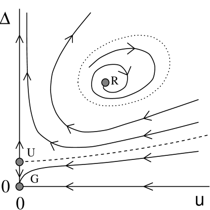
FIG. 2.: Schematic flow diagram on the critical surface for $p<p_{c}$ and $d>4$ (but $d<d^{*}$, see the text). The dotted line separates the region of attraction for the Random FP (R) from a region of runaway flow. Both the Random FP and the Gaussian FP (G) are stable, while the Unphysical FP (U) is unstable. The broken line is a separatrix that marks the limit of the region of attraction of the Gaussian FP.

For $p<p_{c}$ (with $p_{c}=16\epsilon_{\tau}/(4\epsilon_{\tau}-3\epsilon)$ in one-loop approximation), the Random FP is stable and has a finite region of attraction. With increasing distance of the initial values from the FP we still found the flow to be attracted by the FP, but only after oscillatory excursions to large values of $\Delta$ and $u$, where the one-loop approximation is no longer valid. It is natural to interpret these large excursion as runaway flow indicative of the RS phase. This interpretation gets support from the two-loop flow equations derived by Boyanovsky and Cardy[9]. Solving these equations for $d<4$, with a reinterpretation of the parameters as appropriate for the present problem, we have found that the region of attraction for the Random FP is finite, with a limit cycle separating the region of attraction from a region of runaway flow. We conclude that the flow diagram on the critical surface ($t=t^{*}$) is qualitatively as shown in Figs. 2, 3. For $d>4$, both the Gaussian FP and the Random FP are stable. The former is attractive for small values of $\Delta$, and its region of attraction is limited by a separatrix that ends in the unstable Unphysical FP, see Fig. 2. For disorder values above that separatrix the flow is qualitatively the same as in $d<4$. These flow diagrams correspond to the phase diagrams discussed above and shown for $d<4$ in Fig. 1. We finally discuss the general structure of the phase diagram, in particular why LRO occurs only in a disorder window. As we have seen, the nontrivial structure of the phase diagram arises from competition between fluctuation induced LRO, and LM. Technically, the instanton or LM contribution to the free energy goes like $-\Delta^{\alpha}$, with $\alpha$ some positive exponent. For small bare values of $\Delta$, the instanton scale $b_{c}\sim\Delta^{-1/\epsilon}$ is large, and it takes many RG iterations to reach it. The renormalized $\Delta$ is therefore large, and the free energy gain due to the formation of LM is larger than that due to forming LRO. The same is true for large bare values of $\Delta$. However, for intermediate disorder values LRO is energetically favorable. The approach to the AFM FP then leads to a large correlation length, i.e. long-ranged spin-spin correlations that fall off only as $1/r^{d-2+\eta}$. Such long-ranged correlations quench the LM [15], which is why the rare regions discussed in Ref. [6] cannot preclude the AFM transition.

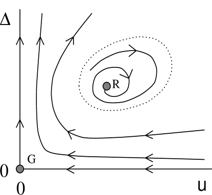
FIG. 3.: Same as Fig. 2, but for $d<4$.

In summary, we have found that long-range order in $3-d$ disordered AFM systems can be restored by quantum fluctuations which destroy the random-singlet phase. Our most striking prediction is the possibility of re-entry into an AFM state with increasing disorder. Any attempts to check this prediction experimentally, however, should keep in mind that changing the disorder usually also changes other parameters, e.g. $J$ and $u$. One might also try to confirm our result by looking for a transition between an antiferromagnetic and a random-singlet phase with exponents that are neither mean-field like (as at $T=0$ in the clean case), nor classical (as at $T>0$ in the disordered case)[16]. Although the present theory has been formulated for itinerant electrons, this could be done in either metallic or insulating systems.

This work was supported by the NSF under grant Nos. DMR-92-17496 and DMR-95-10185. We greatfully acknowledge the hospitality of the TSRC in Telluride, CO.

REFERENCES

- [1] For a recent review, see, e.g., D. Belitz and T. R. Kirkpatrick, Rev. Mod. Phys. 66, 261 (1994).
- [2] S. Chakravarty, B. I. Halperin, and D. R. Nelson, Phys. Rev. B 39, 2344 (1989).
- [3] S. Sachdev, A. V. Chubukov, and A. Sokol, Phys. Rev. B, 51, 14874 (1995).
- [4] R. N. Bhatt and P. A. Lee, Phys. Rev. Lett. 48, 344 (1982).
- [5] C. Dasgupta and S. K. Ma, Phys. Rev. B 22, 1305 (1980).
- [6] R. N. Bhatt and D. S. Fisher, Phys. Rev. Lett. 68, 3072 (1992).
- [7] At large disorder one also expects a metal-insulator transition with a critical disorder . The position of with respect to and can not be determined a priori and may depend on the system. Before is reached the system may enter a Griffiths phase with nontrivial magnetic properties, D. Belitz and T. R. Kirkpatrick, Phys. Rev. B xx, xxx (1995).
- [8] J. A. Hertz, Phys. Rev. B 14, 1165 (1976).
- [9] Such a double expansion is necessary for a controlled perturbative description of the fluctuation effects. It has been used to treat classical magnets with correlated impurities, S. N. Dorogovtsev, Phys. Lett. 76A, 169 (1980). D. Boyanovsky and J. L. Cardy, Phys. Rev. B 26, 154 (1982) gave an improved treatment of this model and also noted its relevance for quantum systems.
- [10] See, e.g., S. K. Ma, Modern Theory of Critical Phenomena, (Benjamin, Reading, MA 1976).
- [11] See, e.g., G. Grinstein in Fundamental Problems in Statistical Mechanics VI, edited by E. G. D. Cohen (North Holland, Amsterdam 1985), p.147.
- [12] A. B. Harris, J. Phys. C 7, 1671 (1974). E. R. Korutcheva and D. I. Uzunov, Phys. Lett. 106A, 175 (1984); A. J. Millis, Phys. Rev. B 48, 7183 (1993); and Sachdev, Chubukov, and Sokol (Ref. [3]), have mentioned the instability of any Hertz-type fixed point against disorder. Korutcheva and Uzunov have also discussed certain aspects of the model, Eq. (3). Notice that disorder has a much more profound effect at than at . For instance, for a clean classical 3D Heisenberg model the exponent , and hence the clean FP is stable against disorder. More generally, thermal fluctuations at are not as easily overcome by disorder as are quantum fluctuations. In general, they suppress the RS phase and enable LRO AFM to exist.
- [13] D. E. Khmelnitskii, Phys. Lett. 67A, 59 (1978).
- [14] See, e.g., J. Zinn-Justin, Quantum Field Theory and Critical Phenomena, Clarendon (Oxford 1989), ch. 35.
- [15] See Eq. (9.17b) in Ref. [1].
- [16] In an actual experiment at one will always observe a crossover to classical exponents sufficiently close to the transition.