Ferromagnetism in Hubbard Models

Abstract

We present the first rigorous examples of non-singular Hubbard models which exhibit ferromagnetism at zero temperature. The models are defined in arbitrary dimensions, and are characterized by finite-ranged hoppings, dispersive bands, and finite on-site Coulomb interaction $U$. The picture, which goes back to Heisenberg, that sufficiently large Coulomb interaction can revert Pauli paramagnetism into ferromagnetism has finally been confirmed in concrete examples.

Department of Physics, Gakushuin University, Mejiro, Toshima-ku, Tokyo 171, JAPAN

Introductions:

The origin of ferromagnetism has been a mystery in physical science for quite a long time [1]. It was Heisenberg [2] who first realized that ferromagnetism is intrinsically a quantum many-body effect, and proposed a scenario that spin-independent Coulomb interaction and the Pauli exclusion principle generate “exchange interaction” between electronic spins. One of the motivations to study the so-called Hubbard model has been to establish and understand the generation of ferromagnetism in simplified situations [3, 4]. Unfortunately, rigorous examples of ferromagnetism (or ferrimagnetism) in the Hubbard models have been limited to singular models which have infinitely large Coulomb interaction (Nagaoka-Thouless ferromagnetism [5]), or in which magnetization is supported by a dispersionless band (Lieb’s ferrimagnetism [6], and flat-band ferromagnetism due to Mielke [7] and the present author [8]). In [9, 10], local stability of ferromagnetism in a generic family of Hubbard models with nearly-flat bands was proved.

In the present Letter, we treat a class of Hubbard models in arbitrary dimensions, which are non-singular in the sense that they have finite ranged hoppings, dispersive (single-electron) bands, and finite Coulomb interaction $U$. We prove that the models exhibit ferromagnetism in their ground states provided that $U$ is sufficiently large. We recall that Hubbard models with dispersive bands (like ours) exhibit Pauli paramagnetism when $U=0$, and remain non-ferromagnetic for sufficiently small $U$. The appearance of ferromagnetism is a purely non-perturbative phenomenon.

As far as we know, this is the first time that the existence of ferromagnetism is established in non-singular itinerant electron systems. We stress that our examples finally provide the definite affirmative answer to the long standing fundamental problem; whether spin-independent Coulomb interaction can be the origin of ferromagnetism in itinerant electron systems [11]. See [8, 10, 12] for further discussions on ferromagnetism in the Hubbard models.

Main results:

In order to simplify the discussion, we describe our results in one-dimensional models. We discuss models in higher dimensions at the end of the Letter. Let $N$ be an arbitrary integer, and let $\Lambda$ be the set of integers $x$ with $|x|\leq N$. We identify $x=-N$ and $x=N$ to regard $\Lambda$ as a periodic chain with $2N$ sites. We denote by ${\cal E}$ and ${\cal O}$ the subsets of $\Lambda$ consisting of even and odd sites (integers), respectively. As usual we denote by $c^{\dagger}_{x,\sigma}$, $c_{x,\sigma}$, and $n_{x,\sigma}$ the creation, the annihilation, and the number operators, respectively, for an electron at site $x\in\Lambda$ with spin $\sigma=\uparrow,\downarrow$.

We consider the standard Hubbard Hamiltonian

$$H=\mathop{\sum_{x,y\in\Lambda}}_{\sigma=\uparrow,\downarrow}t_{x,y}\,c^{\dagger}_{x,\sigma}c_{y,\sigma}+U\sum_{x\in\Lambda}n_{x,\uparrow}n_{x,\downarrow},$$ (1)

where $t_{x,x+1}=t_{x+1,x}=t^{\prime}$ for any $x\in\Lambda$, $t_{x,x+2}=t_{x+2,x}=t$ if $x\in{\cal E}$, $t_{x,x+2}=t_{x+2,x}=-s$ if $x\in{\cal O}$, and $t_{x,x}=V$ if $x\in{\cal O}$. The remaining elements of $t_{x,y}$ are vanishing. See Figure 1. Here $s$, $t$, and $U$ are positive parameters [13]. The parameters $t^{\prime}$ and $V$ are determined by $s$, $t$, and another positive parameter $\lambda$ as $t^{\prime}=\lambda(s+t)$ and $V=(\lambda^{2}-2)(s+t)$. Our main theorem applies to the case $\lambda=\sqrt{2}$, where we have $V=0$. We consider the Hilbert space with $N$ electrons in the system. This corresponds to the quarter-filling of the whole bands, or the half-filling of the lower band.

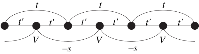
Figure 1: The one-dimensional lattice and the hopping matrix elements. There are hoppings to nearest and next-nearest neighbors, and on-site potential.

If we consider the single-electron problem corresponding to the Hamiltonian (1), we find that the model has two bands with dispersion relations $\varepsilon_{1}(k)=-2s\cos 2k-2(s+t)$, and $\varepsilon_{2}(k)=2t\cos 2k+\lambda^{2}(s+t)$ with $|k|\leq\pi/2$. Note that both the bands have perfect cosine dispersions, which is a special feature of the present model [14]. There is an energy gap $\lambda^{2}(s+t)$ between the two bands.

For $\alpha=1,2,3$, we define the total spin operators by $S^{(\alpha)}_{\rm tot}=\sum_{x\in\Lambda}\sum_{\sigma,\tau=\uparrow,\downarrow}c^{\dagger}_{x,\sigma}\,(p^{(\alpha)}/2)_{\sigma,\tau}\,c_{x,\tau}$, where $p^{(\alpha)}$ are the Pauli matrices, and denote the eigenvalues of $({\bf S}_{\rm tot})^{2}=\sum_{\alpha=1}^{3}(S^{(\alpha)}_{\rm tot})^{2}$ as $S_{\rm tot}(S_{\rm tot}+1)$. The maximum possible value of $S_{\rm tot}$ is $S_{\rm max}\equiv N/2$.

Let $b^{\dagger}_{k,\sigma}$ be the creation operator corresponding to the single-electron eigenstate with the energy $\varepsilon_{1}(k)$. Let $\Phi_{\rm vac}$ be the state with no electrons. The state $\Phi_{\rm ferro}=(\prod_{k}b^{\dagger}_{k,\uparrow})\Phi_{\rm vac}$ (where the lower band is fully filled by up-spin electrons) has the lowest energy among the states with $S_{\rm tot}=S_{\rm max}$. It is easy to observe that $\Phi_{\rm ferro}$ is an eigenstate of $H$ with the energy $E_{0}=-2(s+t)N$. A simple variational calculation shows that $\Phi_{\rm ferro}$ cannot be a ground state of $H$ (and hence the true ground state has $S_{\rm tot}<S_{\rm max}$) if $U<4s$. The main result of the present Letter is the following.

Theorem I—Suppose $\lambda>\lambda_{\rm c}=[(2+\sqrt{5})^{1/2}-2]^{1/2}\simeq 0.241$. If $t/s$ and $U/s$ are sufficiently large, the ground states of the Hamiltonian (1) have $S_{\rm tot}=S_{\rm max}$, and are non-degenerate apart from the $(2S_{\rm tot}+1)$-fold spin degeneracy. $\Phi_{\rm ferro}$ is one of the ground states. How large the parameters should be can be determined by diagonalizing a Hubbard model on a five-site chain. (See Figure 2.)

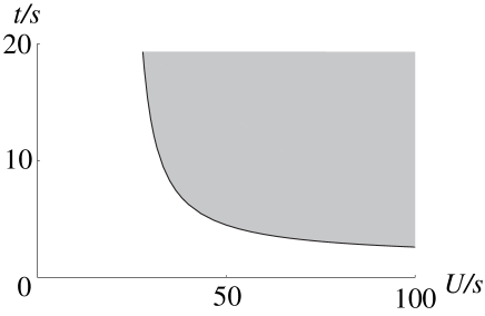
Figure 2: When $\lambda=\sqrt{2}$, Theorem I is applicable for $t/s$ and $U/s$ in the shaded region. The existence of ferromagnetism is established, for examples, if $t\geq 4.5\,s$ when $U=50\,s$, or $t\geq 2.6\,s$ when $U=100\,s$. Though the plot was obtained from a numerical calculation in a five-site Hubbard model, our theorem guarantees that the model with arbitrary lattice size exhibits ferromagnetism.

The present models reduce to the flat-band models studied in [8] if we set $s=0$. Therefore we can regard Theorem I as a confirmation in special cases of the previous conjecture [15, 8, 9, 10] that the flat-band ferromagnetism is stable under perturbations. Moreover the strong result about the spin-wave excitation proved in [9, 10] also applies to the preset models.

Theorem II—Suppose that the model parameters satisfy $\lambda\geq\lambda_{3}$, $s/t\leq\rho_{0}$, and $K_{2}\lambda t\geq U\geq A_{3}\lambda^{2}s$, where $\lambda_{3}$, $\rho_{0}$, $K_{2}$, and $A_{3}$ are positive constants that appear in [10]. Then the spin-wave excitation energy $E_{\rm SW}(k)$ (i.e., the lowest energy among the states with $(N-1)$ up-spin electrons and one down-spin electron and with crystal momentum $k$) of the Hubbard model (1) satisfies

$$F_{2}\frac{4U}{\lambda^{4}}(\sin k)^{2}\leq E_{\rm SW}(k)-E_{0}\leq F_{1}\frac{4U}{\lambda^{4}}(\sin k)^{2},$$ (2)

where $E_{0}$ is the ground state energy, and $F_{1}$, $F_{2}$ are constants such that $F_{1}\simeq F_{2}\simeq 1$ if $\lambda\gg 1$, $\lambda s\ll t$, and $U\gg\lambda^{2}s$. (See [10] for details and a proof.)

In the parameter region where both Theorems I and II are applicable, we have an ideal situation that the global stability of ferromagnetism as well as the appearance of “healthy” low-lying excited states are established rigorously. We have rigorously derived a ferromagnetic system with (effective) exchange interaction $J\simeq 2U/\lambda^{4}$, starting from the Hubbard models for itinerant electrons!

It is quite likely that the present models represent (Mott-Hubbard) insulators. We expect that the same models with smaller electron numbers describe metallic ferromagnetism [16], but have no rigorous results in this direction (except for those in the flat-band models [8]).

Proof of Theorem I:

For $x\in\Lambda$ and $\sigma=\uparrow,\downarrow$, we define $a_{x,\sigma}=\lambda\,c_{x,\sigma}-(-1)^{x}(c_{x-1,\sigma}+c_{x+1,\sigma})$, which correspond to the strictly localized basis states used in [8, 9, 10]. The anti-commutator $\{a^{\dagger}_{x,\sigma},a_{y,\sigma}\}$ is $\lambda^{2}+2$ if $x=y$, is $1$ if $|x-y|=2$, and is vanishing otherwise. By using these operators, Hamiltonian (1) can be written in a compact manner as

$$H=(\lambda^{2}s-2t)N-s\mathop{\sum_{x\in{\cal E}}}_{\sigma=\uparrow,\downarrow}a^{\dagger}_{x,\sigma}a_{x,\sigma}+t\mathop{\sum_{x\in{\cal O}}}_{\sigma=\uparrow,\downarrow}a^{\dagger}_{x,\sigma}a_{x,\sigma}+U\sum_{x\in\Lambda}n_{x,\uparrow}n_{x,\downarrow},$$ (3)

in the sector with $N$ electrons. We further rewrite it as $H=(\lambda^{2}s-2t)N+\sum_{x\in{\cal E}}h_{x}$ with the local Hamiltonian defined as

$$h_{x}=-s\sum_{\sigma=\uparrow,\downarrow}a^{\dagger}_{x,\sigma}a_{x,\sigma}+U\,n_{x,\uparrow}n_{x,\downarrow}+\sum_{r=\pm 1}\left(\frac{t}{2}\sum_{\sigma=\uparrow,\downarrow}a^{\dagger}_{x+r,\sigma}a_{x+r,\sigma}+\frac{U}{2}\,n_{x+r,\uparrow}n_{x+r,\downarrow}\right).$$ (4)

Since $[h_{x},h_{x+2}]\neq 0$, it is impossible to diagonalize all $h_{x}$ simultaneously.

Lemma—Suppose $\lambda>\lambda_{\rm c}$, and $t/s$ and $U/s$ are sufficiently large. Then the minimum eigenvalue of $h_{x}$ (regarded as an operator on the whole Hilbert space) is $-(\lambda^{2}+2)s$. In any of the corresponding eigenstates, there are one, two, or three electrons in the sublattice $\{x-2,x-1,x,x+1,x+2\}$, and these electrons are coupled ferromagnetically. Any eigenstate $\Phi$ with the eigenvalue $-(\lambda^{2}+2)s$ can be written in the form

$$\Phi=a^{\dagger}_{x,\uparrow}\Phi_{1}+a^{\dagger}_{x,\downarrow}\Phi_{2},$$ (5)

with some states $\Phi_{1}$ and $\Phi_{2}$, and satisfies

$$c_{x+1,\downarrow}c_{x+1,\uparrow}\Phi=0.$$ (6)

We prove the Lemma in the next part. In what follows, we assume that the model parameters satisfy the conditions in the Lemma. The basic strategy of the proof of Theorem I is to extend the local ferromagnetism found above into a global ferromagnetism. Special characters of the present model makes such an extension possible.

The Lemma implies $h_{x}\geq-(\lambda^{2}+2)s$, and hence $H\geq(\lambda^{2}s-2t)N-N(\lambda^{2}+2)s=-2(s+t)N=E_{0}$. This proves that $\Phi_{\rm ferro}$ (which has the eigen-energy $E_{0}$) is a ground state.

To show the uniqueness of the ground states, we assume $\Phi$ is a ground state, i.e., $H\Phi=E_{0}\Phi$. Then we have $h_{x}\Phi=-(\lambda^{2}+2)s\,\Phi$ for each $x\in{\cal E}$, and $\Phi$ is characterized by the Lemma. We note that the collection of states $(\prod_{x\in A}a^{\dagger}_{x,\uparrow})(\prod_{x\in B}a^{\dagger}_{x,\downarrow})\Phi_{\rm vac}$ with arbitrary subsets $A,B\subset\Lambda$ such that $|A|+|B|=N$ forms a (complete) basis of the $N$-electron Hilbert space. Imagine that we expand $\Phi$ using this basis. Since (5) holds for any $x\in{\cal E}$, $\Phi$ must be written in the form

$$\Phi=\sum_{\tilde{\sigma}}\varphi(\tilde{\sigma})(\prod_{x\in{\cal E}}a^{\dagger}_{x,\sigma(x)})\Phi_{\rm vac},$$ (7)

where $\tilde{\sigma}=(\sigma(x))_{x\in{\cal E}}$ is a spin configuration with $\sigma(x)=\uparrow,\downarrow$, and $\varphi(\tilde{\sigma})$ is a coefficient. Unlike in the flat-band models [8], a state of the form (7) is not necessarily an eigenstate of the hopping part of $H$.

By examining how $c_{x+1,\downarrow}c_{x+1,\uparrow}$ acts on (7), the condition (6) reduces to

$$\varphi(\tilde{\sigma})=\varphi(\tilde{\sigma}_{x,x+2}) \tilde{\sigma}$$ for any , (8)

where $\tilde{\sigma}_{x,x+2}$ is the spin configuration obtained by switching $\sigma(x)$ and $\sigma(x+2)$ in $\tilde{\sigma}$. Since (8) holds for any $x\in{\cal E}$, we find that $\varphi(\tilde{\sigma})=\varphi(\tilde{\tau})$ whenever $\sum_{x\in{\cal E}}\sigma(x)=\sum_{x\in{\cal E}}\tau(x)$. Since $\Phi_{\rm ferro}$ is written as $\Phi_{\rm ferro}={\rm const.}(\prod_{x\in{\cal E}}a^{\dagger}_{x,\uparrow})\Phi_{\rm vac}$, this means that $\Phi$ can be written in the form $\Phi=\sum_{M=0}^{N}\alpha_{M}(S^{-}_{\rm tot})^{M}\Phi_{\rm ferro}$, where the spin lowering operator is $S^{-}_{\rm tot}=\sum_{x\in\Lambda}c^{\dagger}_{x,\downarrow}c_{x,\uparrow}$. This proves that $\Phi_{\rm ferro}$ and its $SU(2)$ rotations are the only ground states of $H$.

Proof of Lemma:

Because of the translation invariance, it suffices to prove the Lemma for $x=0$. We first diagonalize the hopping part of $h_{0}$ (obtained by setting $U=0$). We express a single-electron state supported on the sublattice $\Lambda_{0}=\{-2,-1,0,1,2\}$ as a five-dimensional vector $\varphi=(\varphi_{-2},\varphi_{-1},\varphi_{0},\varphi_{1},\varphi_{2})$. The normalized eigenstates are $\varphi^{(0)}=(\lambda^{2}+2)^{-1/2}(0,-1,\lambda,-1,0)$ with the eigenvalue $\varepsilon_{0}=-(\lambda^{2}+2)s$, $\varphi^{(1)}=\{2(\lambda^{2}+1)\}^{-1/2}(\lambda,-1,0,1,-\lambda)$ with $\varepsilon_{1}=0$, $\varphi^{(2)}=\{2(\lambda^{2}+2)(\lambda^{2}+3)\}^{-1/2}(-(\lambda^{2}+2),\lambda,2,\lambda,-(\lambda^{2}+2))$ with $\varepsilon_{2}=0$, and two more with $\varepsilon_{3}=(\lambda^{2}+1)t/2$ and $\varepsilon_{4}=(\lambda^{2}+3)t/2$. We denote the corresponding creation operators as $d^{\dagger}_{i,\sigma}=\sum_{x\in\Lambda_{0}}\varphi^{(i)}_{x}c^{\dagger}_{x,\sigma}$. It is crucial to note that $a^{\dagger}_{0,\sigma}=(\lambda^{2}+2)^{1/2}d^{\dagger}_{0,\sigma}$.

Since the local Hamiltonian $h_{0}$ conserves the number of electrons in $\Lambda_{0}$, we can examine its minimum eigenvalue in each sector with a fixed number of electrons in $\Lambda_{0}$. When there are no electrons in $\Lambda_{0}$, the only possible eigenvalue of $h_{0}$ is $0>-(\lambda^{2}+2)s$. Let $f_{n}$ and $e_{n}$ be the minimum eigenvalues of $h_{0}$ in the sectors with $n$ electrons in $\Lambda_{0}$ with the total spin (of the $n$ electrons) $S^{(n)}_{\rm tot}=n/2$, and $S^{(n)}_{\rm tot}<n/2$, respectively.

Noting that $f_{n}=\sum_{m=0}^{n-1}\varepsilon_{m}$, we find $f_{1}=f_{2}=f_{3}=-(\lambda^{2}+2)s$ and $f_{n}>-(\lambda^{2}+2)s$ for $n\geq 4$. Since the corresponding ferromagnetic eigenstates are $(\prod_{m=0}^{n-1}d^{\dagger}_{m,\uparrow})\widetilde{\Phi}$ (where $\widetilde{\Phi}$ is an arbitrary state with no electrons in $\Lambda_{0}$) or their $SU(2)$ rotations, they are written in the desired form (5), and satisfy (6). Therefore, in order to prove the Lemma, it suffices to show

$$e_{n}>-(\lambda^{2}+2)s n=2,3,\ldots,8$$ for any . (9)

Since the condition (9) only involves eigenvalues of a finite system, it can be checked by numerically diagonalizing finite dimensional matrices for given values of $\lambda$, $s$, $t$ and $U$. We can thus construct a computer aided proof that our Hubbard model exhibits ferromagnetism. Figure 2 summarizes the result of a preliminary analysis in this direction.

Let us prove (9) in a range of parameters without using computers. Let $e_{2}^{\rm sym}$ (resp., $e_{2}^{\rm as}$) be the minimum eigenvalue of $h_{0}$ in the sector with two electrons in $\Lambda_{0}$ forming spin-singlet states which is symmetric (resp., antisymmetric) under the spatial reflection $x\rightarrow-x$. Let us evaluate $e_{2}^{\rm sym}$. In the limit $t\uparrow\infty$, a spin-singlet state with two electrons in the symmetric sector which has finite expectation value of $h_{0}$ is written as

$$\Psi=\left\{\alpha\,d^{\dagger}_{0,\uparrow}d^{\dagger}_{0,\downarrow}+\frac{\beta}{\sqrt{2}}(d^{\dagger}_{0,\uparrow}d^{\dagger}_{2,\downarrow}+d^{\dagger}_{2,\uparrow}d^{\dagger}_{0,\downarrow})+\gamma\,d^{\dagger}_{2,\uparrow}d^{\dagger}_{2,\downarrow}+\delta\,d^{\dagger}_{1,\uparrow}d^{\dagger}_{1,\downarrow}\right\}\widetilde{\Phi},$$ (10)

where $\widetilde{\Phi}$ is any state with no electrons in $\Lambda_{0}$. The expectation value of the hopping part of $h_{0}$ in this state is given by $\langle h_{0}^{\rm hop}\rangle=(\Psi,h_{0}^{\rm hop}\,\Psi)/(\Psi,\Psi)=A[-2(\lambda^{2}+2)s|\alpha|^{2}-(\lambda^{2}+2)s|\beta|^{2}]$, where $A=(|\alpha|^{2}+|\beta|^{2}+|\gamma|^{2}+|\delta|^{2})^{-1}$. If we further let $U\uparrow\infty$, a finite energy state must also satisfy $c_{0,\downarrow}c_{0,\uparrow}\Psi=0$ and $c_{1,\downarrow}c_{1,\uparrow}\Psi=0$. These conditions lead us to the constraints

$$\frac{\lambda^{2}}{\lambda^{2}+2}\alpha+\frac{2\lambda}{(\lambda^{2}+2)\sqrt{\lambda^{2}+3}}\beta+\frac{2}{(\lambda^{2}+2)(\lambda^{2}+3)}\gamma=0,$$

$$\frac{1}{\lambda^{2}+2}\alpha-\frac{\lambda}{(\lambda^{2}+2)\sqrt{\lambda^{2}+3}}\beta+\frac{\lambda^{2}}{2(\lambda^{2}+2)(\lambda^{2}+3)}\gamma+\frac{1}{2(\lambda^{2}+1)}\delta=0.$$ (11)

We denote the desired minimum eigenvalue $e_{2}^{\rm sym}$ for $t=U=\infty$ as $e_{2,\infty}^{\rm sym}$. To get $e_{2,\infty}^{\rm sym}$, we minimize the energy expectation value $\langle h_{0}^{\rm hop}\rangle$ with respect to the constraints (11). The rest is a tedious but straightforward estimate. Eliminating $\beta$ from (11), we get $\alpha+\gamma/(\lambda^{2}+3)+\delta/(\lambda^{2}+1)=0$, which implies $|\gamma|^{2}+|\delta|^{2}\geq f(\lambda)|\alpha|^{2}$ with $f(\lambda)=\{(\lambda^{2}+1)^{-2}+(\lambda^{2}+3)^{-2}\}^{-1}$. By substituting this bound into $\langle h_{0}\rangle+(\lambda^{2}+2)s=A(\lambda^{2}+2)s(-|\alpha|^{2}+|\gamma|^{2}+|\delta|^{2})$, we get $e_{2,\infty}^{\rm sym}+(\lambda^{2}+2)s\geq A(\lambda^{2}+2)s|\alpha|^{2}\{f(\lambda)-1\}$. Noting that $\alpha\neq 0$ in the minimizer, the condition $f(\lambda)>1$ (which is equivalent to $\lambda>\lambda_{\rm c}$) implies $e_{2,\infty}^{\rm sym}>-(\lambda^{2}+2)s$. Since $e_{2}^{\rm sym}$ is a continuous function of $t$ and $U$, this proves that $e_{2}^{\rm sym}>-(\lambda^{2}+2)s$ for sufficiently large $t$ and $U$.

By repeating the similar (but easier) variational analysis, we find that $e_{2}^{\rm as}=-(\lambda^{2}/3)s>-(\lambda^{2}+2)s$, and $e_{n}=\infty$ for $n\geq 3$ when $t=U=\infty$. This implies that the desired condition (9) holds for $\lambda>\lambda_{\rm c}$ and sufficiently large $t$ and $U$. The Lemma has been proved.

Models in higher dimensions:

Models in higher dimensions can be constructed and analyzed in quite the same spirit [12]. Take, for example, the flat-band models studied in [8]. ($V$ and $M$ correspond to ${\cal E}$ and ${\cal O}$ of the present paper, respectively.) For $x\in V$ we let $a_{x,\sigma}$ as in [8]. For $x=m(v,w)\in M$, we let $a_{x,\sigma}=\lambda c_{x,\sigma}+c_{v,\sigma}+c_{w,\sigma}$. We define the Hamiltonian as

$$H=-s\mathop{\sum_{x\in V}}_{\sigma=\uparrow,\downarrow}a^{\dagger}_{x,\sigma}a_{x,\sigma}+t\mathop{\sum_{x\in M}}_{\sigma=\uparrow,\downarrow}a^{\dagger}_{x,\sigma}a_{x,\sigma}+U\sum_{x\in\Lambda}n_{x,\uparrow}n_{x,\downarrow},$$ (12)

which again contains next-nearest neighbor hoppings and on-site potentials. (12) should be compared with (3). By a straightforward extension of the present method, we can prove that the ground states of the model with $|V|$-electrons exhibit ferromagnetism when $\lambda$, $t/s$, and $U/s$ are sufficiently large [12].

It is a pleasure to thank Tohru Koma, Andreas Mielke, and Bruno Nachtergaele for useful discussions.

Note added (August 1997): The proof of Theorem I has been considerably improved. Now the condition $\lambda>\lambda_{\rm c}$ has been replaced simply by $\lambda\neq 0$. Full details will appear in [12], which is still under preparation for the moment.

References

• [*] Electronic address: hal.tasaki@gakushuin.ac.jp
• [1] D. C. Mattis, The Theory of Magnetism I (Springer-Verlag, 1981).
• [2] W. J. Heisenberg, Z. Phys. 49, 619 (1928).
• [3] For a recent survey of rigorous results in the Hubbard model, see E. H. Lieb, in Proceedings of “Advances in dynamical systems and quantum physics”, World Scientific (in press), and in Proceedings of 1993 NATO ASW “The physics and mathematical physics of the Hubbard model”, Plenum (in press).
• [4] Recently Müller-Hartmann [J. Low. Temp. Phys. 99, 349 (1995)] argued that the Hubbard model with $U=\infty$ on a one-dimensional zigzag chain exhibits ferromagnetism. Since the model is away from half-filling, $U=\infty$ does not necessarily mean that the model is singular. Although his argument is quite interesting, it does not form a mathematically rigorous proof (as far as we can read off from his paper) as it involves an uncontrolled continuum limit of a strongly interacting system. Interestingly, the geometry of the chain is exactly the same as that of ours.
• [5] Y. Nagaoka, Phy. Rev. 147, 392 (1966); D. J. Thouless, Proc. Phys. Soc. London 86, 893 (1965).
• [6] E. H. Lieb, Phy. Rev. Lett. 62, 1201 (1989).
• [7] A. Mielke, J. Phys. A24, L73 (1991); ibid. A24, 3311 (1991); ibid. A25, 4335 (1992); Phys. Lett. A174, 443 (1993).
• [8] H. Tasaki, Phy. Rev. Lett. 69, 1608 (1992); A. Mielke and H. Tasaki, Commun. Math Phys. 158, 341 (1993).
• [9] H. Tasaki, Phy. Rev. Lett. 73, 1158 (1994).
• [10] H. Tasaki, J. Stat. Phys., 84 535–653 (1996).
• [11] The reader might ask what the basic mechanism of ferromagnetism in the present models is. Our ferromagnetism may be (partially) interpreted in terms either of the standard two pictures of ferromagnetism, namely, the Heisenberg-like “exchange” picture and the band-electron picture. The most crucial point in our proof is that we describe electronic states in such a way that both the particle-like character of electrons and the band structure of the model are taken into account.
• [12] H. Tasaki, to be published.
• [13] We can of course consider models in which ${\cal E}$-sites and ${\cal O}$-sites have different values of $U$.
• [14] This special property of the dispersion relations is closely related to the representation (3) of the Hamiltonian.
• [15] K. Kusakabe and H. Aoki, Physica B 194–196, 215 (1994); Phy. Rev. Lett. 72, 144 (1994).
• [16] A support to this conjecture is given by a perturbation theory using the Wannier basis. It suggests that the low energy effective theories of these doped models are ferromagnetic $t$-$J$ models, where $|t/J|$ can be made arbitrarily small by taking Hubbard models close to flat-band models.