Quantum phase transitions in spin systems
and
the high temperature limit of continuum quantum field theories

Abstract

We study the finite temperature crossovers in the vicinity of a zero temperature quantum phase transition. The universal crossover functions are observables of a continuum quantum field theory. Particular attention is focussed on the high temperature limit of the continuum field theory, the so-called “quantum-critical” region. Basic features of crossovers are illustrated by a simple solvable model of dilute spinless fermions, and a partially solvable model of dilute bosons. The low frequency relaxational behavior of the quantum-critical region is displayed in the solution of the transverse-field Ising model. The insights from these simple models lead to a fairly complete understanding of the system of primary interest: the two-dimensional quantum rotor model, whose phase transition is expected to be in the same universality class as those in antiferromagnetic Heisenberg spin models. Recent work on the experimental implications of these results for the cuprate compounds is briefly reviewed.

Proceedings of the
19th IUPAP International Conference on Statistical Physics
Xiamen, China, July 31 - August 4 1995
World Scientific, to be published, edited by B.-L. Hao.

I Introduction

Consider a quantum system on an infinite lattice described by the Hamiltonian ${\cal H}(g)$, with $g$ a dimensionless coupling constant. For any reasonable $g$, all observable properties of the ground state of ${\cal H}$ will vary smoothly as $g$ is varied. However, there may be special points, like $g=g_{c}$, where there is a non-analyticity in some property of the ground state: we identify $g_{c}$ as the position of a quantum phase transition. In finite lattices, non-analyticities can only occur at level crossings; the possibilities in infinite systems are richer as avoided level crossings can become sharp in the thermodynamic limit. In this paper, I will restrict my discussion to second order quantum transitions, or transitions in which the correlation length and correlation time diverge as $g$ approaches $g_{c}$. As I will review below, any such quantum transition can be used to define a continuum quantum field theory (CQFT): the CQFT has no intrinsic short-distance (or ultraviolet) cutoff. The main purpose of this paper is to review some recent work [1, 2, 3, 4, 5] on the properties of ${\cal H}(g)$ at finite temperatures ($T$) in the vicinity of $g=g_{c}$. This is equivalent to a study of the finite $T$ crossovers of the associated CQFT. We shall focus especially on the dynamic properties of a ubiquitous finite $T$ region, usually called “quantum critical” [6] (as we shall see below, there are reasons why this name is misleading and not quite appropriate; nevertheless, I will use it here). The quantum-critical region appears as the high $T$ limit of the CQFT; unlike the statics of classical lattice models, the high $T$ limit of a CQFT is usually highly non-trivial. All of this discussion will take place in the context of some simple examples drawn from quantum spin systems.

I set the stage by reviewing the Wilsonian approach to critical phenomena and field theories [7], using the perspective of quantum critical phenomena. By the usual Trotter product decomposition, we can set up the partition function of ${\cal H}(g)$ as a functional integral over degrees of freedom which fluctuate as a function of the spatial co-ordinate $x$ and imaginary time $\tau$. Let us now examine the behavior of this functional integral under the rescaling transformation [8, 9]

$$x\rightarrow e^{-\ell}x~{}~{}~{}~{}~{}~{}~{}~{}~{}~{}~{}\tau\rightarrow e^{-z\ell}\tau$$ (1)

The dynamic exponent $z$ determines the relative scaling dimensions of space and time co-ordinates. The critical point at $g=g_{c}$ is a fixed point of (1), and $g-g_{c}$ is a relevant perturbation away from this point. We have therefore the flow equation

$$\frac{dg}{d\ell}=\frac{1}{\nu}(g-g_{c})$$ (2)

which defines the critical exponent $\nu$. (For simplicity I do not discuss the case of fixed points with more than one relevant perturbation, as they can be treated in a similar manner). In the long-distance, long-time limit, this deviation from the critical point will be characterized by some renormalized energy scale, $G$. I emphasize that $G$ is a dimensionful parameter, expressed in the laboratory units of energy, and directly measurable in an experiment; a typical example would be an energy gap. In the vicinity of the critical point, the renormalized energy scale $G$ will be related to the bare coupling $g$ by

$$G\sim\Lambda|g-g_{c}|^{z\nu}$$ (3)

where $\Lambda$ is an ultraviolet cutoff, measured for convenience in the units of energy too. From the perspective of a field theorist, the CQFT associated with the quantum critical point is now defined by taking the limit $\Lambda\rightarrow\infty$ at fixed $G$; from (3) we see that, because $z\nu>0$, it is possible to take this limit by tuning the bare coupling $g$ closer and closer to the critical point as $\Lambda$ increases. (A condensed matter physicist would take the complementary, but equivalent, perspective of keeping $\Lambda$ fixed but moving closer to criticality by lowering his probe frequency $\omega\sim G$). The resulting CQFT then contains only the energy scale $G$. At finite temperatures, there is a second energy scale $T$ (using units in which $k_{B}=1$); its thermodynamic properties will then be a universal function of the only dimensionless ratio available—$G/T$. It is the purpose of this paper to review recent work on the crossovers as a function of $G/T$ in a number of systems, and to highlight the unusual properties of the heretofore unexplored high-temperature, “quantum critical”, limit of the CQFT, $T\gg G$.

It is now easy to see why the high $T$ limit of the CQFT can be non-trivial. A conventional high $T$ expansions of the lattice model ${\cal H}$ proceeds with the series

$$\mbox{Tr}e^{-{\cal H}/T}=\mbox{Tr}1-\frac{1}{T}\mbox{Tr}{\cal H}+\frac{1}{2T^{2}}\mbox{Tr}{\cal H}^{2}+\ldots$$ (4)

The successive terms in this series are well-defined and finite because of the ultraviolet cutoffs provided by the lattice. Further, the series is well-behaved provided $T$ is larger than all other energy scales; in particular we need $T\gg\Lambda$. In contrast, the CQFT was defined by the limit $\Lambda\rightarrow\infty$ at fixed $T$, $G$, so the high $T$ limit of the CQFT corresponds to the intermediate temperature range $G\ll T\ll\Lambda$ of the lattice model. It is not possible to access this temperature range by an expansion as simple as (4), and more sophisticated techniques, to be discussed here, are necessary. (One could also, of course, determine a large number of terms in (4) and then use some Padé extrapolation methods to access the $T\ll\Lambda$ region: this method has been used by Sokol et. al. [10] and I will not discuss it here).

In contrast to the static properties, the dynamic properties of ${\cal H}$ are already non-trivial in the high $T\gg\Lambda$ limit of the lattice model. Although one expects some sort of incoherent, dissipative dynamics, the damping co-efficients cannot be determined directly—all the approaches used so far are essentially variants of the methods discussed by Moriya [11] and Forster [12], and use a short-time expansion, coupled with an ansatz for the spectral function, to extrapolate to the long-time limit. In this paper, we will discuss the dynamics in the high $T$ limit of the CQFT, $G\ll T\ll\Lambda$, or the “quantum-critical dynamics”. The dynamics continues to be dissipative and relaxational, but is not amenable to a description either by a classical Boltzmann equation for a dilute gas of quasiparticle excitations, or by a classical Langevin-like models of the types discussed in the classic review of Hohenberg and Halperin [13]. However, as we shall show, the scaling structure of the CQFT does permit some progress to be made; indeed we will discuss below the complete solution of the quantum-critical dynamics of a simple spin model, including the exact determination of a damping co-efficient.

We will begin our discussion with a simple solvable model of spinless fermions in Section II: this will allow introduction of the main concepts in a very simple setting. Section III will extend these results to a related but more complex model of dilute bosons in spatial dimensions $d<2$. An explicit solution of the relaxational dynamics of the quantum-critical region will be obtained in the discussion in Section IV on the Ising model in a transverse field. The expository analyses of these toy models will lead in Section V to the main system of interest—the $O(3)$ quantum rotor model in $d=2$. We will also review applications of these results to numerical simulations and experiments. Finally Section VI will conclude by highlighting the main results and noting recent work on related subjects.

II Dilute gas of spinless fermions

Much of the physics I wish to discuss is displayed in a surprisingly simple model of a dilute gas of spinless fermions at finite temperature: its scaling forms have a structure identical to those of much more complicated models. The main shortcoming of the model is that the associated CQFT has no interactions, and there is therefore no relaxational behavior in the scaling functions.

Consider the following Hamiltonian:

$${\cal H}_{F}=-t\sum_{<ij>}\left(c_{i}^{\dagger}c_{j}+c_{j}^{\dagger}c_{i}-c_{i}^{\dagger}c_{i}-c_{j}^{\dagger}c_{j}\right)-\mu\sum_{i}c_{i}^{\dagger}c_{i}$$ (5)

where $c_{i}$ is a spinless fermion annihilation operator at the site $i$ of a $d$-dimensional hypercubic lattice, and $<ij>$ are nearest neighbors. There are no interactions in ${\cal H}_{F}$, so it is trivially solvable. Consider the ground state of ${\cal H}_{F}$ as a function of the dimensionless coupling constant $g=\mu/t$. For $g<g_{c}=0$, the ground state has no particles. There is a non-analytic onset in the density of particles at $g=g_{c}$, signaling a quantum phase transition. The bandwidth $\sim t$ of the fermions plays the role of the upper cutoff in energy ($\Lambda$) for this transition, and the critical region defining the applicability of a CQFT is roughly $T,\mu\ll t$. In fact, it is not difficult to determine the exact effective action of the CQFT (in units with $\hbar=1$):

$${\cal L}_{F}=\int d^{d}x\int_{0}^{1/T}d\tau\Psi_{F}^{\dagger}(x,\tau)\left(\frac{\partial}{\partial\tau}-\frac{\nabla^{2}}{2m}-\mu\right)\Psi_{F}(x,\tau)$$ (6)

where $\Psi_{F}(x_{i})=a^{-d}c_{i}$, $m\sim 1/(ta^{2})$, and $a$ is the lattice spacing. For this action we can identify by the usual methods the exponents $\nu=1/2$ and $z=2$ at the $\mu=0$ critical point; taking the density $n=\langle\Psi_{F}^{\dagger}\Psi_{F}\rangle$ as the order parameter, we get the exponents $\beta=d/2$ and $\eta=d$. Further, it is also easy to see that all interactions are irrelevant at this critical point in all dimensions $d>0$ (the least irrelevant interaction term, $|\Psi_{F}\nabla\Psi_{F}|^{2}$, becomes relevant only for $d<0$). Finally, for the renormalized energy scale measuring the deviation from the critical point, $G$, we may take $G=\mu$, the bare chemical potential in ${\cal H}_{F}$. Note that there is no non-universal scale-factor in the relationship between $G$ and $\mu$—this is a consequence of the triviality of the critical exponents. More typical models with anomalous exponents will have non-universal scale-factors.

We show in Fig 1 the phase diagram of ${\cal H}_{F}$ as a function of $G=\mu$ and $T$. Our interest is primarily in the regions within the hatched lines where the CQFT (6) applies. Within this region there are three physically distinct types of behavior (A, B and C): as ${\cal L}_{F}$ is trivially solvable, the universal properties of A, B, and C and the crossovers between them can be exactly determined. Let us describe the regions in turn:

(A) Activated $\mu\ll-T$: The fermions are very dilute, with a density $\sim e^{\mu/T}$. Quantum effects are suppressed and the particles behave classically.

(B) Fermi or Luttinger liquid $\mu\gg T$: Now quantum degeneracy effects are paramount. At $T=0$, the ground state is a Fermi liquid (in $d=1$, a Luttinger liquid); at finite $T$ thermal effects lead to a small number of particle and hole excitations near the Fermi surface.

(C) Quantum Critical $|\mu|\ll T$: Unlike A and B, the temperature $T$ is the most important energy scale in this region. We can set $\mu=0$ here without much damage (all corrections involve positive powers of $\mu/T$). The energy of a typical excitation in this region is of order $T$ and as a result, quantum and thermal fluctuations are equally important.

The relationships between the regions becomes clearer upon considering an explicit example of a crossover function. The density of particles $n=\langle\Psi_{F}^{\dagger}\Psi_{F}\rangle$ obeys the scaling form

$$n=(2mT)^{d/2}\Phi_{n}\left(\frac{\mu}{T}\right)$$ (7)

where the universal scaling function $\Phi_{n}(\overline{\mu})$ is given by

$$\Phi_{n}(\overline{\mu})=\int\frac{d^{d}k}{(2\pi)^{d}}\frac{1}{e^{k^{2}-\overline{\mu}}+1}.$$ (8)

Notice that there are no arbitrary scale-factors in (7). In the activated region A ($\overline{\mu}\ll-1$), we have $\Phi_{n}\approx e^{\overline{\mu}}/(4\pi)^{d/2}$, which is exactly the result we would have obtain from the classical Maxwell-Boltzmann statistics. In the Fermi liquid region B ($\overline{\mu}\gg 1$), $\Phi_{n}\approx\overline{\mu}^{d/2}V_{d}/(2\pi)^{d}$, where $V_{d}$ is the volume of the unit sphere in $d$ dimensions; this is the fully quantum result obtained by filling up the Fermi sphere. Most interesting is the quantum critical region C ($|\overline{\mu}|\ll 1)$ where

$$\Phi_{n}(\overline{\mu})=\zeta\left(\frac{d}{2}\right)\left(\frac{\pi}{2}\right)^{d}\left(1-2^{1-d/2}\right)+{\cal O}(\overline{\mu})$$ (9)

The value of $\Phi_{n}(0)$ depends upon the details of the Fermi distribution function, and not just its forms in the classical and quantum limits: this illustrates our assertion that quantum and classical effects are equally important in region C.

It is also interesting to compare the behavior of the density in the universal region C with the true high temperature limit of the lattice model - region D. In other words, we are going vertically upwards in $T$ at $\mu=0$ in Fig 1. It is easy to compute:

$$n=\left\{\begin{array}[]{cc}(2mT)^{d/2}\Phi_{n}(0)&|G|\ll T\ll\Lambda~{}~{}(\mbox{region C})\\ 1/2a^{d}-c_{1}/T&T\gg\Lambda~{}~{}(\mbox{region D})\end{array}\right.$$ (10)

where $c_{1}$ is a non-universal constant (recall that in this model $G=\mu$ and $\Lambda=t$). Notice the difference between the universal high $T$ limit of the CQFT (the first result) and the lattice high $T$ limit. I hope that this example has illustrated the general principle, and in the remainder of the paper I will make no further reference to non-universal regions like D. It will be implicitly assumed that we are working with the universal continuum theory, and we will describe only regions like A, B and C.

Before closing our discussion on this deceptively simple model, we discuss the scaling form of observables as a function of momentum $k$ and frequency $\omega$. Because of the absence of interactions, the single-particle Green’s function is trivial; so we discuss the density-density correlator $\chi_{n}(k,\omega)$ which has a slightly more interesting structure. As the particles are free, $\chi_{n}$ is of course given simply by the Lindhard function, which can be manipulated into the scaling form

$$\chi_{n}(k,\omega)=\frac{(2mT)^{d/2}}{T}\Phi_{\chi_{n}}\left(\frac{k}{\sqrt{2mT}},\frac{\omega}{T},\frac{\mu}{T}\right)$$ (11)

where $\Phi_{\chi_{n}}$ is a universal complex-valued function related to the Lindhard function. Notice that, like the scaling form (7), there are again no arbitrary scale factors. Further, $\Phi_{\chi_{n}}$ is well-defined at $\mu/T=0$, where it yields the dynamic susceptibility of the quantum-critical region C. We will see several other examples of scaling forms like (7) and (11) in this paper, but the scaling functions will not be as simple as they are here.

III Dilute Bose gas

Now we consider the same density onset quantum transition considered in Sec II, but for the case of bosons. The discussion here is drawn from that of Sachdev, Senthil and Shankar [4] to which the reader is referred for further details.

Unlike the case for spinless fermions, it is no longer possible to ignore the interactions between the particles. We consider the properties of the following continuum model

$${\cal L}_{B} = \int d^{d}x\int_{0}^{1/T}d\tau\Psi_{B}^{\dagger}(x,\tau)\left(\frac{\partial}{\partial\tau}-\frac{\nabla^{2}}{2m}-\mu\right)\Psi_{B}(x,\tau)$$ (12)

$$+ \frac{1}{2}\int d^{d}x\int d^{d}x^{\prime}\int_{0}^{1/T}d\tau|\Psi_{B}(x,\tau)|^{2}v(x-x^{\prime})|\Psi_{B}(x^{\prime},\tau)|^{2}$$ (13)

where $\Psi_{B}$ is a boson annihilation operator, and $v(x)$ is a repulsive interaction of range $\sim a$. Like ${\cal L}_{F}$, ${\cal L}_{B}$ has a quantum phase transition at $\mu=T=0$, and we will discuss its universal properties here. Because of the finite range of $v$, the universality only sets in at distances larger than $a$. A straightforward RG analysis [14] of the vicinity of the quantum critical point shows that $v$ flows into the $v=0$ fixed point for $d\geq 2$. It turns out that $v$ is actually dangerously irrelevant for $d\geq 2$: we do not wish to enter into a discussion of such effects here, and so most of our remaining discussion will be restricted to $d<2$.

For $d<2$, $v(x)$ flows into a universal fixed point interaction $v(x)=u^{\ast}\delta(x)$ for some $d$ dependent constant $u^{\ast}$. The scaling structure of this fixed point turns out to be very closely related to the non-interacting spinless fermion model of Sec II for the same value of $d$. All exponents and scaling forms of the boson and fermion models are identical, but the scaling functions themselves are different. The crossover phase diagram of the $d<2$ dilute Bose gas is essentially identical to the fermion phase diagram in Fig 1, but the physical interpretation of the phases is somewhat different:

(A) Activated $\mu\ll-T$: This is essentially identical to the fermion case as the particles are dilute and their quantum statistics plays a negligible role.

(B) Incipient Superfluid $\mu\gg T$: The ground state is now a superfluid (in $d=1$ a Luttinger liquid), but classical thermal fluctuations destroy the long range order at any non-zero temperature. Nevertheless, the phase coherence length is large and system behaves like a superfluid at short scales.

(C) Quantum Critical $|\mu|\ll T$: This is similar to the fermion case in that $T$ is the most important energy scale. However, there are now strong interactions among the particles, leading to an incoherent excitation spectrum. The system does not display characteristics of a superfluid ground state at any length scale, but instead crosses over directly from free particle behavior at short time scales, to dissipative, relaxational dynamics at long time scales. The single particle Green’s function $G(x,\tau)=\langle\Psi_{B}(x,\tau)\Psi_{B}^{\dagger}(0,0)\rangle$ has a non-trivial scaling function $\Phi_{G}$ (this form actually holds in all three regions A, B, and C)

$$G^{R}(k,\omega)=\frac{1}{T}\Phi_{G}\left(\frac{k}{\sqrt{2mT}},\frac{\omega}{T},\frac{\mu}{T}\right).$$ (14)

We have Fourier transformed and analytically continued to the retarded Green’s function at real frequencies. This scaling form also holds for the spinless fermions of Section II, but the scaling function then is simply the free fermion form $\Phi_{G}(\overline{k},\overline{\omega},\overline{\mu})=1/(\overline{\omega}-\overline{k}^{2}-\overline{\mu}+i\eta)$ where $\eta$ is a positive infinitesimal. Computing $\Phi_{G}$, and other scaling functions, for bosonic quantum critical dynamics is not as easy. One approach [4] is to expand in powers of the fixed-point interaction $u^{\ast}$ which becomes small as $d$ approaches 2 from below: this becomes an expansion in $\varepsilon=2-d$.

In $d=1$, it is possible to make more explicit progress. It has been argued [4] that now $u^{\ast}=\infty$. The bosons thence become impenetrable, and their quantum mechanics becomes identical to those of free fermions. Hence, in $d=1$, the quantum critical dynamics of dilute gases of spinless fermions and boson are described by the same CQFT, ${\cal L}_{F}$ of Eqn (6). For the bosonic system we have to supplement ${\cal L}_{F}$ with the following non-local relationship between the boson and fermion operators (essentially a continuum Jordan-Wigner transformation)

$$\Psi_{B}(x)=\exp\left(i\pi\int_{-\infty}^{x}dx^{\prime}\Psi_{F}^{\dagger}(x^{\prime})\Psi_{F}(x^{\prime})\right)\Psi_{F}(x)$$ (15)

We are not home yet, as evaluating correlators of (15) under (6) is not easy. Korepin and Slavnov [15, 16] have succeeded in showing how this problem may be reduced to determining the solution and Fredholm determinant of a linear Fredholm integral equation. At this stage, numerical analysis is required, and some scaling functions have been determined to essentially arbitrary accuracy [4].

Finally, an additional comment about the $d\geq 2$ case. There is now true superfluidity and a finite temperature phase transition to a normal state, all within region B. The remainder of the phase diagram remains the same as in the $d\leq 2$ case.

IV Ising Model in a transverse field

Unlike the dilute Fermi and Bose gases, the Ising model possesses anomalous exponents. Yet it is simple enough in $d=1$ to allow exact computation of a quantum-critical dynamic correlation function. We will also review, in this section, the very useful and general mapping between the quantum model and an equivalent classical statistical mechanics model; we will then discuss the crossovers in the phase diagram like Fig 1 in the context of the classical model. Some of of the following discussion is a review of well-known properties of the Ising model [17, 18, 19, 20]; our main purpose here is to use the explicit solution in $d=1$ to present a physical interpretation which generalizes to other quantum phase transitions.

We will explicitly discuss the following Hamiltonian, describing the Ising model in a transverse field in $d=1$ (we will remark briefly on the generalization to higher $d$):

$${\cal H}_{I}=-J\sum_{i}\left(g\sigma_{x,i}+\sigma_{z,i}\sigma_{z,i+1}\right)$$ (16)

where $J>0$ in an overall energy scale, $g>0$ is a dimensionless coupling constant, and $\sigma_{x,i},\sigma_{z,i}$ are Pauli matrices on a chain of sites, $i$. Consider the ground states of ${\cal H}_{I}$ for small and large $g$ in turn. For small $g$, the second term in (16) dominates and the spins all align themselves either in the $+z$ or $-z$ directions: there is a spontaneous magnetization and spin-reversal symmetry is broken. On the other hand, for large $g$, the first term in (16) prefers a state which is in a superposition of $\sigma_{z}$ eigenstates, with different sites uncorrelated: the wavefunction looks like $\prod_{i}(|+\rangle_{i}+|-\rangle_{i})$. These two limits are separated by a phase transition at $g=g_{c}$ (in fact, $g_{c}=1$, exactly, because of a self-duality property of (16)). In this section, we shall discuss the finite $T$ dynamic properties in the vicinity of $g=g_{c}$.

To begin, we recall the well-known fact [17, 18] that the $T=0$ correlators of ${\cal H}_{I}$ are similar to those in the classical, two-dimensional, Ising model given by the partition function $\mbox{Tr}~{}e^{-F}$ with

$$F=-K\sum_{<ij>}\sigma_{z,i}\sigma_{z,j}$$ (17)

where the sites $i,j$ now lie on a square lattice (say). This classical model has a phase transition at $K=K_{c}$. At the level of the critical continuum theories, the mapping between the classical and quantum models become exact [18]. There is a simple relationship between the two-dimensional field theory, with classical degrees of freedom, describing $F$ in the vicinity of $K=K_{c}$ and the one-dimensional quantum field theory describing ${\cal H}_{I}$ near $g=g_{c}$: one simply identifies one of the spatial directions of the classical theory as an imaginary time, and then analytically continues the correlators to real time, to obtain observables of the quantum theory. This mapping leads immediately to some useful information. As the classical theory is spatially isotropic, the quantum theory has dynamic exponent $z=1$. Further, in the classical model the $\sigma_{z}~{}\sigma_{z}$ correlator behaves like $\sim p^{-7/4}$ in momentum space [19] ($p$ is the two-dimensional momentum of the classical model); analytically continuing this to real time, we obtain for the dynamic susceptibility $\chi(k,\omega)$ (this is the $\sigma_{z}~{}\sigma_{z}$ correlator of the quantum ${\cal H}_{I}$ and $k$ is now a one-dimensional spatial momentum) as a function of $d=1$ momentum $k$ and frequency $\omega$:

$$\chi(k,\omega)=\frac{Z}{(c^{2}k^{2}-\omega^{2})^{7/8}}~{}~{}~{}~{}~{}~{}T=0,g=g_{c}.$$ (18)

Here $Z$ and $c$ (an excitation velocity) are non-universal constants. We plot $\mbox{Im}\chi(k,\omega)/\omega$ in Fig 2. Notice that there are no delta functions in the spectral density, indicating the absence of any well-defined quasiparticles. Instead, we have a critical continuum of excitations. We can also compute the dynamic local susceptibility,

$$\chi_{L}^{\prime\prime}(\omega)=\int\frac{dk}{2\pi}\mbox{Im}\chi(k,\omega),$$ (19)

a quantity often measured in neutron scattering experiments:

$$\chi_{L}^{\prime\prime}(\omega)=\mbox{sgn}(\omega)\frac{\sqrt{\pi}Z}{2\Gamma(7/8)\Gamma(5/8)c}\left(\frac{1}{|\omega|}\right)^{3/4}~{}~{}~{}~{}~{}~{}T=0,g=g_{c}.$$ (20)

This quantity is the density of states of local spin-flip excitations, and has a divergence as $\omega\rightarrow 0$.

Our discussion so far has been at $T=0$, and let us turn now to non-zero $T$. A finite $T$ translates into a finite size $L_{\tau}=1/T$ for the classical model along imaginary time direction. Periodic boundary conditions are imposed along the finite direction, and so the classical model has the geometry of a cylinder with circumference $L_{\tau}=1/T$. We now discuss the crossovers at finite $T$ in the context of the classical model. At $L_{\tau}=\infty$ ($T=0$) we can characterize the deviations from criticality by the correlation length $\xi\sim|g-g_{c}|^{-1}$ (for the quantum model we may choose our renormalized energy scale $G=1/\xi\sim|g-g_{c}|$). At distances shorter than $\xi$, the spins display critical correlations characteristic of the point $K=K_{c}$; it is only at distances larger than $\xi$ that they become sensitive to the value of $K-K_{c}$ and display characteristics of the ordered (for $K>K_{c}$) or the paramagnetic (for $K<K_{c}$) phase. Now consider the effect of a finite $L_{\tau}$; there are two distinct possibilities:

(i) $\xi<L_{\tau}$ (for the quantum model, $T<G$): Moving from the shortest to largest length scales, the crossover from critical to non-critical (either ordered or paramagnetic) behavior still occurs at a scale $\sim\xi$; the length scale $L_{\tau}$ has little effect at this point. The effects of $L_{\tau}$ only become apparent at larger scales, at which point it is permissible to use an effective model which characterizes the non-critical ground state.

(ii) $L_{\tau}<\xi$ (for the quantum model, $T>G$): Now the short-distance critical fluctuations see a finite size $L_{\tau}$ before they have had a chance to become sensitive to $K-K_{c}$. These critical fluctuations are quenched by finite size effects in a universal way. The resulting non-critical theory then responds only weakly at the scale $\xi$. Note that the system does not display characteristics of the ordered or the paramagnetic state, of the $L_{\tau}=\infty$ system, at any length scale.

The above arguments are summarized in Figs 4 and 4; notice that Fig 4 is quite similar to Fig 1. In all three regions of Fig 4, at the largest frequencies, $\omega$, ${\cal H}_{I}$ displays the critical correlations of the $g=g_{c}$ point as depicted in Fig 4 (we have returned now to the language of the quantum model ${\cal H}_{I}$).

In regions A and B there is a crossover from these critical fluctuations, at an energy scale $G$, to the behavior of the ordered ($g<g_{c}$) or paramagnetic ($g>g_{c}$) ground state of ${\cal H}_{I}$ (see Fig 4). Both ground states have a gap, and thermal fluctuations will lead to dilute gas of quasiparticle excitations. We expect that an effective classical model (like Glauber [21] dynamics, which is similar in spirit to the Langevin models of Hohenberg and Halperin [13]) will provide a suitable description of these thermal fluctuations. In $d=1$, on the ordered side ($g<g_{c}$), these quasiparticle excitations are the ‘kink’ and ‘anti-kink’ solitons; even an infinitesimal concentration of these is sufficient to destroy long-range order at any finite temperature. However, for $d>1$, long-range order is not immediately destroyed: as a result there is finite temperature phase transition within region A where the magnetic moment disappears; this transition will be in the universality class of the $d$-dimensional classical Ising model [17].

In the quantum-critical region C, the critical fluctuations are quenched by thermal effects at the energy scale $T$ (see Fig 4; an early analysis of finite $T$ crossovers in the transverse-field Ising model by Suzuki [17] failed to identify region C). This quenching is completely universal and will be described explicitly below. The system has had no chance to display any characteristic of either non-critical ground state at any frequency scale. At low frequencies, the system realizes a new quantum relaxational regime. It is this regime which is really characteristic of the region C, and not the high frequency critical behavior which is present in all three regions. It is in this sense that the name “quantum-critical” of region C is a misnomer.

As in the case of the dilute Fermi and Bose gases considered earlier, the dynamic susceptibility $\chi(k,\omega)$ will satisfy a universal scaling form over the regions of Fig 4:

$$\chi(k,\omega)=\frac{Z}{T^{7/4}}\Phi_{\chi}\left(\frac{ck}{T},\frac{\omega}{T},\frac{G}{T}\right)$$ (21)

In the following we will determine the leading term in $\Phi_{\chi}$ in the quantum-critical region C i.e. we will present an exact expression for $\Phi_{\chi}(\overline{k},\overline{\omega},0)$.

In the classical model $F$ at $K=K_{c}$ and $L_{\tau}=\infty$, we know from (18) that the Green’s function $G(x,\tau)=\langle\sigma_{z}(0,0)\sigma_{z}(x,\tau)\rangle\sim(x^{2}+\tau^{2}c^{2})^{-1/8}$; we are using the label $\tau$ for spatial direction corresponding to imaginary time. We can now use a remarkable result of Cardy [22], which relies on the conformal invariance of this critical theory, to obtain an exact result for $G$ in a system with a finite $L_{\tau}$:

$$G(x,\tau)=\frac{\Gamma(1/8)Z}{2^{13/8}\pi^{3/4}\Gamma(7/8)c}\left(\frac{1}{L_{\tau}}\right)^{1/4}\left(\frac{1}{\cosh(2\pi x/L_{\tau}c)-\cos(2\pi\tau/L_{\tau})}\right)^{1/8}$$ (22)

This result has been asserted earlier by an inspection of the partial differential equation satisfied by $G$ [23]. Although results like (22) have been known to conformal field theorists for some time, they usually interchange the roles of $x$ and $\tau$ i.e. they consider systems of finite spatial length $L_{x}$, and infinite temporal length, so that the system is in its ground state. For us, the spatial extent is infinite, and there is a finite length $L_{\tau}$ along the $\tau$ direction, with the correlator (22) periodic in $\tau$ with period $L_{\tau}$ (such a perspective has also been discussed by Shankar [24] and by Korepin et. al. [16]). Note that it doesn’t really make sense to talk about the long imaginary time limit, $\tau\gg L_{\tau}$. However, after analytic continuation to real time, the long time limit of the quantum problem, $t\gg 1/T$ or $\omega\ll T$, is eminently sensible, and is precisely the new quantum relaxational regime that we wish to access. The analytic continuation is a little more convenient in Fourier space: we Fourier transform (22) to obtain $G(k,\omega_{n})$ at the Matsubara frequencies $\omega_{n}$ and then analytically continue to real frequencies (there are some interesting subtleties in the Fourier transform to $G(k,\omega_{n})$ and its analytic structure in the complex $\omega$ plane, which are discussed elsewhere [4]). This gives us the universal function $\Phi_{\chi}$ in the quantum-critical region:

$$\Phi_{\chi}(\overline{k},\overline{\omega},0)=\frac{1}{(4\pi)^{7/4}}\frac{\displaystyle\Gamma\left(\frac{1}{16}+i\frac{\overline{\omega}+\overline{k}}{4\pi}\right)\Gamma\left(\frac{1}{16}+i\frac{\overline{\omega}-\overline{k}}{4\pi}\right)}{\displaystyle\Gamma\left(\frac{15}{16}+i\frac{\overline{\omega}+\overline{k}}{4\pi}\right)\Gamma\left(\frac{15}{16}+i\frac{\overline{\omega}-\overline{k}}{4\pi}\right)}.$$ (23)

We show a plot of $\mbox{Im}\Phi_{\chi}/\overline{\omega}$ in Fig 5. This result is the finite $T$ version of Fig 2. Notice that the sharp features of Fig 2 have been smoothed out on the scale $T$, and there is non-zero absorption at all frequencies. We can also observe the crossover as a function of frequency claimed earlier in Fig 4. Notice that for $\overline{\omega},\overline{k}\gg 1$ there is a well-defined peak in $\mbox{Im}\Phi_{\chi}/\overline{\omega}$ (Fig 5) rather like the $T=0$ critical behavior of Fig 2. However, for $\overline{\omega},\overline{k}\ll 1$ we cross-over to the quantum relaxational regime and the spectral density $\mbox{Im}\Phi_{\chi}/\overline{\omega}$ is similar to a Lorentzian around $\overline{\omega}=0$. This relaxational behavior can be characterized by a relaxation rate $\Gamma_{R}$ defined as [13]

$$\Gamma_{R}^{-1}=-i\left.\frac{\partial\ln\chi(0,\omega)}{\partial\omega}\right|_{\omega=0};$$ (24)

(this is motivated by the phenomenological relaxational form $\chi(0,\omega)=\chi_{0}/(1-i\omega/\Gamma_{R}+{\cal O}(\omega^{2}))$). From (21) and (23) we determine:

$$\Gamma_{R}=\left(2\tan\frac{\pi}{16}\right)\frac{k_{B}T}{\hbar},$$ (25)

where we have returned to physical units. The ease with which this result was obtained belies (I claim) its remarkable nature. Notice that we are working in a closed Hamiltonian system, evolving unitarily in time with the operator $e^{-i{\cal H}_{I}t}$, from an initial density matrix given by the Gibbs ensemble at a temperature $T$. Yet, we have obtained relaxational behavior at low frequencies, and determined an exact value for a dissipation constant. Such behavior is more typically obtained in phenomenological models which couple the system to an external heat bath and postulate an equation of motion of the Langevin type. Notice also that ${\cal H}_{I}$ in (16) is known to be integrable with an infinite number of conservation laws [18]. However, the conservation laws are associated with a mapping to a free fermion model and are highly non-local in our $\sigma_{z}$ degrees of freedom; they play essentially no role in our considerations, and do not preclude relaxational behavior in the $\sigma_{z}$ variables.

For completeness we also present results on a related observable which shows the crossover from critical to quantum relaxation behavior. We consider the local susceptiblity $\chi_{L}^{\prime\prime}$, and obtain the finite $T$ form of (20) by integrating (23) over momenta:

$$\chi_{L}^{\prime\prime}(\omega) = \frac{Z}{cT^{3/4}}\Phi_{L}\left(\frac{\omega}{T},\frac{G}{T}\right)$$ (26)

$$\Phi_{L}(\overline{\omega},0) = \frac{1}{2^{7/4}\pi^{5/4}\Gamma(5/8)\Gamma(7/8)}\sinh\left(\frac{\overline{\omega}}{2}\right)\left|\Gamma\left(\frac{1}{8}-i\frac{\overline{\omega}}{2\pi}\right)\right|^{2}$$ (27)

A plot of the scaling function $\Phi_{L}$ is shown in Fig 6. The function has the asymptotic limits:

$$\Phi_{L}(\overline{\omega},0)=\left\{\begin{array}[]{cc}\displaystyle\frac{\Gamma^{2}(1/8)}{2^{11/4}\pi^{5/4}\Gamma(5/8)\Gamma(7/8)}\overline{\omega}&|\overline{\omega}|\ll 1\\ \displaystyle\mbox{sgn}(\overline{\omega})\frac{\sqrt{\pi}}{2\Gamma(7/8)\Gamma(5/8)}\left(\frac{1}{|\overline{\omega}|}\right)^{3/4}&|\overline{\omega}|\gg 1\end{array}\right.$$ (28)

The small $\overline{\omega}$ behavior is relaxational as $\Phi_{L}$ is linear in frequency, and the critical behavior at large frequencies agrees with (20).

V Quantum rotors in two dimensions

The study of this model is of direct experimental interest, as it is believed [6] to be a reasonable model of the spin fluctuations in antiferromagnetic compounds like $La_{2}CuO_{4}$ and its lightly doped variants. The insight gained from the simple models studied in the previous sections will now be of great use, and we will rapidly be able to present a scaling analysis of its quantum phase transition.

The Hamiltonian of the quantum rotor model is

$${\cal H}_{R}=J\sum_{i}\frac{g}{2}\vec{L}_{i}^{2}-J\sum_{<ij>}\vec{n}_{i}.\vec{n}_{j}$$ (29)

where $J>0$ is an overall energy scale, $g>0$ is a dimensionless coupling constant, and $i$,$j$ are the sites of a two dimensional lattice ($<ij>$ denotes nearest neighbors). Notice the similarity between the forms of ${\cal H}_{R}$ and ${\cal H}_{I}$ in (16): it will turn out that the corresponding terms play a similar role. On each site $i$ of the lattice we have the 3-component vector operators $\vec{L}$, $\vec{n}$ (dropping the site index), which obey the commutation relations:

$$[n_{a},n_{b}]=0~{}~{},~{}~{}[L_{a},n_{b}]=i\epsilon_{abc}n_{c}~{}~{},~{}~{}[L_{a},L_{b}]=i\epsilon_{abc}L_{c}.$$ (30)

The vector $\vec{n}$ is of unit length $\vec{n}^{2}=1$, and its orientation identifies direction of the local magnetic order; the quantum rotor model is usually considered as an effective model for an underlying system of Heisenberg spins—in this case the magnetic order can be any ordering which is specified by a single vector and has no spatially averaged magnetic moment. The simplest example of this is the two sublattice Néel ordering, and we will therefore refer to $\langle\vec{n}\rangle$ as the Néel order parameter. The $\vec{L}$ operator measures the angular momentum, and as all phases have no net magnetic moment, we will always have $\langle\vec{L}\rangle=0$.

For further insight into the meaning of ${\cal H}_{R}$, consider the eigenstates of a single site Hamiltonian $Jg\vec{L}^{2}/2$. This describes a particle moving on a unit sphere with angular co-ordinate $\vec{n}$ and kinetic energy $Jg\vec{L}^{2}/2$. Its eigenenergies are $Jg\ell(\ell+1)/2$ with degeneracy $2\ell+1$ where $\ell=0,1,2,3\ldots$. The ground state is a non-degenerate singlet ($\ell=0$) and has maximum uncertainty in the orientation of $\vec{n}$. For large $g$, the ground state of ${\cal H}_{R}$ can be approximated by the tensor product of $\ell=0$ states on each site. This state is clearly a quantum paramagnet and has a gap, $\Delta$, to all excitations. Notice the similarity between this state and the large $g$ quantum paramagnet of the Ising model ${\cal H}_{I}$; in both cases the order parameters $\sigma_{z}$, $\vec{n}$ are in a state of maximum uncertainty. The small $g$ limit of ${\cal H}_{R}$ is also similar to the small $g$ limit of ${\cal H}_{I}$: now the exchange interactions between the sites prefer a state in which $\vec{n}$ has the same definite orientation on each site. Therefore, we expect long-range Néel order in the small $g$ ground state. These two limiting states will be separated by a quantum phase transition at $g=g_{c}$, which is, of course, the main subject of interest in this section.

Before discussing the critical properties, we pause to remark on the relationship between the rotor model and Heisenberg antiferromagnets. Consider a pair of antiferromagnetically coupled spin-$S$ Heisenberg spins: the eigenstates of this pair will have energies $\propto\ell(\ell+1)-\mbox{const}$ for $\ell=0,1,\ldots 2S$. Notice the similarity between these states and those of a single quantum rotor; the only difference is that there is no upper limit on the maximum value of $\ell$ in the rotor case. However, it is reasonable to expect that these extra high energy states will not modify the low energy properties of lattice models. Therefore, there is little reason to doubt that the critical properties of Heisenberg antiferromagnets with a natural pairing of spins (or more generally, a natural clustering into an even number of spins) will be same as those of the rotor model. Antiferromagnets with no such pairing contain net Berry phase terms in their imaginary time path integral, beyond those present for the rotor model. However these Berry phases cancel between the sites, except for “hedgehog”-like spacetime singularities [25], and it has been argued [1, 3] that these remnant Berry phases have no effect of the leading critical singularities. The reader is referred to the original papers for further discussion on these subtle issues [26, 3]: we will restrict our discussion here to the much simpler rotor model ${\cal H}_{R}$.

The critical properties and phase diagram of the $d=2$ rotor model ${\cal H}_{R}$ turn out to be remarkably similar to those of the transverse field Ising model ${\cal H}_{I}$ of (16) in $d=1$. Like the $d=1$ Ising model, the $d=2$ rotor model has no phase transition at any finite $T$: so the phase diagram of Fig 4 applies to ${\cal H}_{R}$, with no phase boundary in region A (the phase diagram for ${\cal H}_{R}$ in $d=2$ was obtained first by Chakravarty et. al. [6]). In both systems, the $T=0$, $g=g_{c}$ critical point has $z=1$. In the case of ${\cal H}_{I}$ this critical point was described by a CQFT which upon analytic continuation to imaginary time was the field theory of the two-dimensional classical Ising model. The analogous mapping for ${\cal H}_{R}$ yields the CQFT associated with the field theory for the three-dimensional, classical, Heisenberg ferromagnet. The universal scaling functions describing the crossovers in Fig 4 and 4 have an identical form in both theories, although, because the critical field theories are different, the critical exponents, universal amplitude ratios, and scaling functions will have different numerical values. The explicit results presented in Sec IV for quantum-critical region C of the Ising model, all apply, unchanged in form, to the region C of the $d=2$ rotor model: the qualitative features of the spectral functions in Figs 2, 5, and 6 remain the same, and the relaxation rate $\Gamma_{R}$ (defined in (24)) satisfies (25) but with a different universal numerical prefactor. However, unlike the $d=1$ Ising model, we cannot now get exact numerical results for the scaling functions of ${\cal H}_{R}$: this is because the three-dimensional classical Hiesenberg ferromagnet is not exactly solvable (unlike the two-dimensional classical Ising model). Instead we have to be satisfied by approximate methods; reasonably accurate numerical estimates can be obtained in the $1/N$ expansion which has been discussed at length by Chubukov, Sachdev and Ye [3].

There is a small, but significant, difference between the Ising model in $d=1$ and the rotor model in $d=2$ which cannot go unmentioned. This difference applies mainly to “ordered” regime in region A (See Figs 4 and 4). The $T=0$ ground state of ${\cal H}_{I}$ for $g<g_{c}$ has a gap, associate with the finite energy cost of creating a kink or anti-kink soliton. In contrast, the $g<g_{c}$ ground state of ${\cal H}_{R}$ has gapless spin-wave excitations because of the broken continuous $O(3)$ symmetry of the ordered state. So we can no longer use the gap, $\Delta$, as the energy scale, $G=\Delta\sim(g_{c}-g)^{z\nu}$ for measuring deviations from $g=g_{c}$ for $g<g_{c}$. A convenient substitute turns out to be the spin stiffness $G=\rho_{s}$ which has the physical dimensions of energy in $d=2$, and which also vanishes as $\rho_{s}\sim(g_{c}-g)^{z\nu}$. At finite $T$ in region A, it is known [27, 6] that the spin correlation length $\sim\exp(2\pi\rho_{s}/T)$ as $T\rightarrow 0$. It is interesting to note that the behavior of ${\cal H}_{I}$ in $d=1$ is very similar: in this case the correlation length is determined by the mean spacing between kinks, and therefore behaves as $\sim\exp(\Delta/T)$ for low $T$ in region A. (Related to the exponential divergence of the correlation length, there is a further sub-division of the “ordered” regime of region A (Figs 4 and 4) at the energy scale $c/(\mbox{correlation length})$; this complication occurs for both the $d=2$ rotor and the $d=1$ Ising models, and has been discussed elsewhere [3, 6].)

Associated with the continuous $O(3)$ symmetry of ${\cal H}_{R}$, there is an important observable whose properties cannot be deduced by an analogy with the the Ising model. This is the uniform susceptibility $\chi_{H}$, the response to a field, $H$ which couples to the global conserved charge associated with the continuous symmetry:

$${\cal H}_{R}\rightarrow-H\sum_{i}L_{zi}$$ (31)

The scaling dimension of $\chi_{H}$ can be determined exactly using symmetry arguments and the assumption of hyperscaling [2, 5]: this yields the scaling form

$$\chi_{H}=\frac{T}{c^{2}}\Phi_{H}\left(\frac{\rho_{s}}{T}\right)$$ (32)

Here $c$, is the same velocity that appears in a $T=0$ correlator like (18), and $\Phi_{H}$ is a fully universal function. This function was computed exactly [2, 3] in a $O(N=\infty)$ rotor model, along with $1/N$ corrections in some limits; it has the limiting behavior

$$\Phi_{H}(r)=\left\{\begin{array}[]{ll}\displaystyle\frac{\sqrt{5}}{\pi}\ln\left(\frac{\sqrt{5}+1}{2}\right)\left[1-\frac{0.6189}{N}+\ldots\right]+\ldots&r\rightarrow 0\\ \displaystyle\frac{2r}{N}+\frac{N-2}{N}+\ldots&r\rightarrow\infty\end{array}\right.$$ (33)

The two terms in the second result ($r\rightarrow\infty$) are expected to be exact to all orders in $1/N$; the same two terms were also obtained by Hasenfratz and Niedermayer [28]. Notice from (32) and (33) that $\chi_{H}$ has a linear dependence on $T$ both for $T\ll\rho_{s}$ and $T\gg\rho_{s}$; the slopes however differ by a factor of about 3 (for $N=3$) and this will be important for experimental comparisons [2, 3].

A Comparison with simulations and experiments on Heisenberg antiferromagnets

The most straightforward comparison is with the double-layer, spin-1/2 Heisenberg antiferromagnet [29]. This model consists of spin-1/2 Heisenberg spins on two adjacent square lattices, with an intralayer antiferromagnetic exchange $J$ and an interlayer antiferromagnetic exchange $K$. The ratio $K/J$ acts much like the dimensionless coupling $g$, with the large $K/J$ a gapped quantum paramagnet of singlet pairs of spins in opposite layers, and the small $K/J$ magnetically ordered. Extensive numerical simulations have been carried out on this model by Sandvik and collaborators [30], and the critical point $K=K_{c}$ identified rather precisely. It is then possible to study the quantum-critical region C quite carefully as it extends over the maximum $T$ range. A number of universal amplitude ratios, including those associated with $\chi_{H}$, and all results are now in good agreement with the $1/N$ expansion on the $O(N)$ quantum rotor model. Results from high temperature series expansions on the double-layer model also support this conclusion [31].

Secondly, comparisons have been made with the single-layer, square lattice spin-1/2 Heisenberg antiferromagnet, both via simulations and by experimental measurements on $La_{2}CuO_{4}$. This model has long-range order at $T=0$, so must map onto the non-linear sigma model with $g<g_{c}$. The low $T$ region A was studied in the paper of Chakravarty, Halperin and Nelson [6], with good experimental agreement. Here we focus on the issue of whether this lattice model exhibits the CQFT high $T$ behavior of region C, or it goes directly from region A to a non-universal, lattice dominated high $T$ region like D of Fig 4. It was first argued by Chubukov and Sachdev [2] that this model does indeed possess a significant intermediate temperature regime of region C: this was based on comparisons with the $T$ dependence of $\chi_{H}$, with the factor of 3 alluded to above playing an important role. They also noted that it would be difficult to identify this region in the correlation length, an observation that was subsequently re-iterated by Greven et. al. [32]. A rather convincing demonstration of the presence of region C was given recently by Elstner et. al. [31, 10] who examined a large number of observables in a high $T$ expansion, and found good consistency with the universal rotor model results.

Also significant in this context have been nuclear magnetic resonance experiments of Imai et. al. [33] on $La_{2}CuO_{4}$. They have measured the $T$ dependence of the $1/T_{1}$ and $1/T_{2}$ relaxation rates at intermediate temperatures. Their observations are in reasonable agreement with the predictions [2, 3, 34, 35] that can be obtained from the universal scaling result for $\chi(k,\omega)$ in the quantum-critical region C.

VI Conclusions

This paper has presented a discussion of the vicinity of a second-order quantum phase transition in the context of a number of simple models. The overall picture that emerges is summarized in Fig 7, which shows a generic phase diagram in the plane of a coupling constant $g$, and the temperature $T$ of a $d$-dimensional system; this phase diagram is a generalization of a diagram obtained first by Chakravarty et. al. [6] for the $d=2$ quantum rotor model. The quantum phase transition occurs at the point $g=g_{c}$, $T=0$. Associated with this critical point, we can define a continuum quantum field theory (CQFT) over spacetime. In general, space ($x$) and time ($\tau$) do not play a similar role in the CQFT and have different scaling dimensions: $x\rightarrow x/s$, $\tau\rightarrow\tau/s^{z}$ under a spatial rescaling by $s$, with $z$ the dynamic exponent. Further, even in imaginary time, the action for the CQFT can be complex due to the presence of Berry phases, and therefore corresponds to a statistical mechanics model with complex weights. Correlators of the CQFT are the universal functions describing crossovers in the vicinity of $g=g_{c}$, $T=0$. The CQFT has no ultraviolet cutoff, but is characterized solely by two energy scales: the temperature $T$ and an energy scale $G\sim|g-g_{c}|^{z\nu}$ characterizing the deviation of the ground state from the critical point (here $\nu$ is the correlation length exponent). The value of the ratio $G/T$ determines two distinct regions of the CQFT shown in Fig 7. In both regions there is a high frequency regime ($\omega>\mbox{max}(T,G)$) which is dominated by excitations of the critical CQFT of the $g=g_{c}$, $T=0$ point. The regions are distinguished only by their low frequency behavior, which we discuss in turn:

(i) The low $T$ region ($T\ll G$, shown shaded in Fig 7) is a region of “conventional” physics for frequency scales $\omega<G$. This frequency regime can be understood by beginning with the non-critical ground state and examining the particle-like excitations above it. A simple classical model (a Boltzmann equation for a gas of quasiparticle excitations, or a Langevin model of the types discussed by Hohenberg and Halperin [13]) is usually adequate for describing the long-distance, long-time dynamics of these excitations. The shaded region can also contain thermally driven, phase transitions; these transitions will be described by a classical field theory.

(ii) The high $T$ region of the CQFT has a novel quantum relaxational regime. This regime is not described by an effective classical model, and displays intrinsic quantum-mechanical effects at the longest time and distance scales. A scaling analysis for this regime was reviewed in this paper. In some cases, as in the model of Section IV, it is possible to obtain an exact value for the relaxation constant.

This paper has reviewed only a small portion of what is a rapidly developing subject. We list below a number of recent (and not so recent) developments in related areas:

• Quantum transitions between Fermi liquids and states with various types of spin or charge density wave orderings were discussed in important early work by Hertz [8]. He focussed on the immediate vicinity of the finite termperature transition, like that within region A in Fig 4. In particular, Hertz missed the existence of the “quantum-critical” regime (as was pointed out recently by Millis [36]—this oversight is similar to Suzuki’s [17] for the Ising model), which has been the main focus of this paper. More detailed studies of quantum transitions involving Fermi liquids have appeared recently [36, 38, 39, 40, 41, 42]. A related, but different, perspective is provided by studies of critical phenomena in rotor models with doped electrons [43, 39].

• Related ideas on scaling in the quantum critical region have been presented by Tsvelik and collaborators [44].

• A great deal of work has been done recently on “quantum impurity” models [45, 46] like the multi-channel Kondo effect. These models also display quantum phase transitions, with crossovers bearing some similarity to those discussed here. However the transitions do not modify the bulk properties, and are related instead to boundary critical phenomena.

• As we indicated briefly in the discussion on the Bose gas in Section III, dangerously irrelevant operators sometimes need to be considered, as they do in the dilute Bose gas for $d>2$. In fact such effects arise somewhat more frequently than they do in classical critical phenomena, as the upper critical dimension of the quantum transition is often quite low. An early analysis of the dilute Bose gas in $d=3$ by Weichmann et. al. [47] was dominated by such effects, although they did not present their results in the general context of quantum phase transitions. Such a perspective can be found in more recent work [36, 37].

• An important subject, on which much is not understood, is the effect of quenched randomness on quantum phase transitions. An early analysis for the random quantum rotor model was given by Boyanovsky and Cardy [9]. A recent exact solution by Fisher [48] of the random transverse-field Ising model in $d=1$ represents significant progress. The nature of spin glass ordering at $T=0$ and its destruction by quantum fluctuations has also been studied recently [49, 37].

• A number of experiments [50, 51, 52] have reported scaling of the type in Eqn (26) in the local dynamic susceptibility. However the universality classes controlling these systems are not understood and quenched randomness appears to play a significant role. Nevertheless, it is interesting to note the qualitative similarity between the experimental measurements in Fig. 4 of Aronson et. al.[52] and our result for the local susceptibility in Fig 6. The latter measures spin correlations on a single Ising spin induced via its coupling to its environment of other Ising spins. However, there is a fundamental equivalence between the spin being measured and its environment; this is an important difference between our bulk approach and alternative descriptions of the experiments using “quantum impurity” models [45, 46, 52] which clearly distinguish between the impurity and environment degrees of freedom.

• A recent study [53] has examined the CQFT of a quantum ferromagnet. This system does not display a quantum phase transition of the type discussed here. Nevertheless, its phase diagram has regions similar to those in Fig 7 and aspects of its scaling properties are related to those of the dilute Bose gas of Section III.

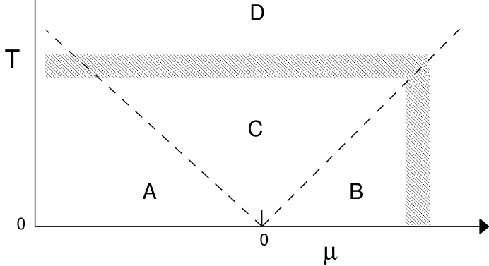
FIG. 1.: Phase diagram of the dilute Fermi gas ${\cal H}_{F}$ (Eqn (5)) as a function of the chemical potential $\mu$ and the temperature $T$. The regions A, B, C, are separated by crossovers; all observables in these regions are described universal crossover functions of the CQFT ${\cal L}_{F}$ (Eqn (6)). Region A has an exponentially activated fermion density, region B is a Fermi liquid (in $d=1$, a Luttinger liquid), and region C is quantum critical. The hatched region marks the boundary of applicability of the CQFT and occurs at $\mu,T\sim\Lambda=t$. The same phase diagram also applies to the dilute Bose gas of Sec. III, but the interpretation of the regions is different.

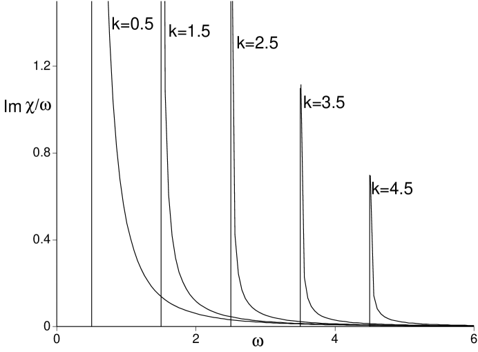
FIG. 2.: Spectral density of the transverse field Ising model (16) at its critical point $g=g_{c}$ at $T=0$. We chose $Z=c=1$ in Eqn (18)

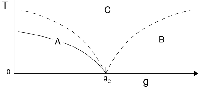
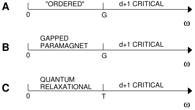
FIG. 3.: Phase diagram of the transverse field Ising model in $d\geq 1$ dimensions; dashed lines denote crossover boundaries, while the solid line is a phase transition. In region A the system displays characteristics of the ordered ground state; thermal fluctuations about this state can destroy long-range order at any non-zero $T$ in $d=1$, but for $d>1$ there is a phase transition (in the universality class of the $d$-dimensional classical Ising model). In region B the system is a gapped quantum paramagnet, and region C is quantum-critical. The crossover boundaries obey $T\sim|g-g_{c}|^{z\nu}$ with $z=1$ and $\nu$ the correlation length exponent of the $d+1$ dimensional classical Ising model ($\nu=1$ in $d=1$). The same phase diagram also applies to the quantum rotor model of Section V in $d\geq 2$, with the difference that the phase transition in region A is present only for $d>2$ and is then in the universality class of the $d+1$ dimensional classical Heisenberg ferromagnet. Chakravarty et. al. [6] obtained this phase diagram for the $d=2$ quantum rotor model.

FIG. 4.: Crossovers as a function of probe frequency in the regions of Fig. 4 for the transverse-field Ising model in $d$ dimensions. The $d+1$ critical regime is described by the CQFT at $g=g_{c}$ and $T=0$. The “ordered” regime is where a classical description in terms of a gas of well-separated domain walls in an otherwise ordered state is appropriate. In $d=1$ such “kinks” destroy long-range-order at any non-zero $T$. The same crossovers also apply to the quantum rotor model of Section V: the “ordered” regime is now one where spin-wave fluctuations about an ordered ground state dominate, and these fluctuations destroy long-range-order at any non-zero $T$ for $d=2$.

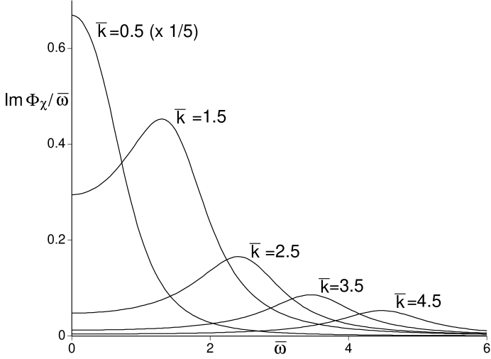
FIG. 5.: Scaling function for the imaginary part of the dynamic susceptibility in the quantum critical region C of the transverse field Ising model in $d=1$. The susceptibility $\chi=Z\Phi_{\chi}/T^{7/4}$ and $\overline{k}=ck/T$, $\overline{\omega}=\omega/T$.

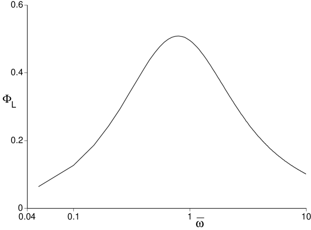
FIG. 6.: Scaling function for the imaginary part of the local dynamic susceptibility in the quantum critical region C of the transverse field Ising model in $d=1$. The susceptibility $\chi_{L}^{\prime\prime}$ is related to $\Phi_{L}$ by (26), $\overline{\omega}=\omega/T$, and notice the logarithmic scale on the horizontal axis.

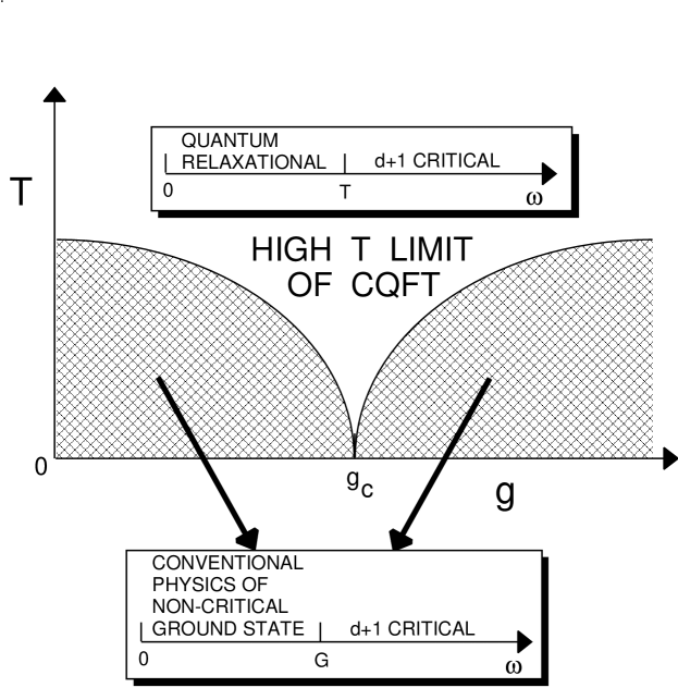
FIG. 7.: Generic phase diagram of a $d$-dimensional system displaying a second-order quantum transition at $g=g_{c}$ and $T=0$. The boundary of the shaded region represents a crossover and not a phase transition. See the text for more information.

- [1] S. Sachdev and J. Ye, Phys. Rev. Lett. 69, 2411 (1992).
- [2] A.V. Chubukov and S. Sachdev, Phys. Rev. Lett. 71, 169 (1993).
- [3] A.V. Chubukov, S. Sachdev, and J. Ye, Phys. Rev. B 49, 11919 (1994).
- [4] S. Sachdev, T. Senthil, and R. Shankar, Phys. Rev. B 50, 258 (1994).
- [5] S. Sachdev, Z. Phys. B 94, 469 (1994).
- [6] S. Chakravarty, B.I. Halperin, and D.R. Nelson, Phys. Rev. B 39, 2344 (1989).
- [7] E. Brezin, J.C. Le Guillou and J. Zinn-Justin, in Phase Transitions and Critical Phenomena, edited by C. Domb and M.S. Green, (Academic Press, New York, 1975) Vol. 6.
- [8] J.A. Hertz, Phys. Rev. B 14, 525 (1976).
- [9] D. Boyanovsky and J.L. Cardy, Phys. Rev. B 26, 154 (1982)
- [10] A. Sokol, R.L. Glenister, and R.R.P. Singh, Phys. Rev. Lett. 72, 1549 (1994).
- [11] T. Moriya, Prog. Theor. Phys. 16, 23 (1956).
- [12] Hydrodynamic Fluctuations, Broken Symmetry, and Correlation Functions, by D. Forster, Benjamin Cummings, Reading (1975).
- [13] P.C. Hohenberg and B.I. Halperin, Rev. Mod. Phys. 49, 435 (1977).
- [14] M.P.A. Fisher, P.B. Weichmann, G. Grinstein, and D.S. Fisher, Phys. Rev. B 40, 546 (1989).
- [15] V.E. Korepin and N.A. Slavnov, Commun. Math. Phys. 129, 103 (1990).
- [16] Quantum Inverse Scattering Method and Correlation Functions by V.E. Korepin, N.M. Bogoliubov, and A.G. Izergin, Cambridge University Press, Cambridge (1993).
- [17] M. Suzuki, Prog. Theor. Phys. 56, 1454 (1976).
- [18] J.B. Kogut, Rev. Mod. Phys. 51, 659 (1979).
- [19] Statistical Field Theory by C. Itzykson and J.-M. Drouffe, Cambridge University Press, Cambridge (1989).
- [20] E. Lieb, T. Schultz, and D. Mattis, Ann. of Phys. 16, 406 (1961); Th. Niemeijer, Physica 36, 377 (1967), 39, 313 (1968); P. Pfeuty, Ann. of Phys. 57, 79 (1970); E. Barouch and B.M. McCoy, Phys. Rev. B 3, 786 (1971); B.M. McCoy, J.H.H. Perk, and R.E. Shrock, Nucl. Phys. B220, 35 (1983).
- [21] R.J. Glauber, J. Math. Phys. 4, 294 (1963).
- [22] J.L. Cardy, J. Phys. A 17, L385 (1984).
- [23] J.H.H. Perk, H.W. Capel, G.R.W. Quispel, and F.W. Nijhoff, Physica 123A, 1 (1984); A. Luther and I. Peschel, Phys. Rev. B 12, 3908 (1975).
- [24] R. Shankar, Int. J. Mod. Phys. B 4, 2371 (1990).
- [25] F.D.M. Haldane, Phys. Rev. Lett. 61, 1029 (1988); N. Read and S. Sachdev, Nucl. Phys. B316, 609 (1989).
- [26] N. Read and S. Sachdev, Phys. Rev. B 42, 4568 (1990).
- [27] E. Brezin and J. Zinn-Justin, Phys. Rev. B 14, 3110 (1976).
- [28] P. Hasenfratz and F. Niedermayer, Phys. Lett. B 268, 231 (1991); Z. Phys. B 92, 91 (1993).
- [29] J. M. Tranquada, G. Shirane, B. Keimer, S. Shamoto, and M. Sato, Phys. Rev. B 40, 4503 (1989); A. J. Millis and H. Monien, Phys. Rev. Lett. 70, 2810 (1993); Phys. Rev. B 50, 16606 (1994).
- [30] A.W. Sandvik and D.J. Scalapino, Phys. Rev. Lett. 72, 2777 (1994); A. W. Sandvik, A.V. Chubukov and S. Sachdev, Phys. Rev. B, 51, 16483 (1995).
- [31] N. Elstner, R.L. Glenister, R.R.P. Singh, and A. Sokol: Phys. Rev. B 51, 8984 (1995).
- [32] M. Greven et. al., Phys. Rev. Lett. 72, 1096 (1994); Z. Phys. B 96, 465 (1995).
- [33] T. Imai et. al. Phys. Rev. Lett. 70, 1002 (1993); ibid 71, 1254 (1993).
- [34] A. Sokol and D. Pines, Phys. Rev. Lett. 71, 2813 (1993).
- [35] A.V. Chubukov, S. Sachdev, and A. Sokol, Phys. Rev. B 49, 9052 (1994).
- [36] A.J. Millis, Phys. Rev. B 48, 7183 (1993).
- [37] S. Sachdev, N. Read and R. Oppermann, Phys. Rev. B, 52, Oct. 1 (1995); cond-mat/9504036.
- [38] L.B. Ioffe and A.J. Millis, cond-mat/9411021; U. Zulicke and A.J. Millis, Phys. Rev. B 51, 8996 (1995); B.L. Altshuler, L.B. Ioffe, and A.J. Millis, cond-mat/9504024.
- [39] S. Sachdev, A.V. Chubukov and A. Sokol, Phys. Rev. B, 51, 14874 (1995).
- [40] S. Sachdev and A. Georges, Phys. Rev. B, 52, Oct. 1 (1995); cond-mat/9503158.
- [41] A.V. Chubukov, cond-mat/9504009.
- [42] G. Murthy and R. Shankar, cond-mat/9505106.
- [43] S. Sachdev Phys. Rev. B 49, 6770 (1994); A.V. Chubukov and S. Sachdev, Phys. Rev. Lett. 71, 3615 (1993).
- [44] B. Andraka and A.M. Tsvelik, Phys. Rev. Lett. 67, 2886 (1991); A.M. Tsvelik and M. Reizer, Phys. Rev. B 48, 9887 (1993).
- [45] I. Affleck and A.W.W. Ludwig, Nucl. Phys. B360, 641 (1991).
- [46] I.E. Perakis, C.M. Varma, and A.E. Ruckenstein, Phys. Rev. Lett. 70, 3467 (1993); C. Sire, C.M. Varma, A.E. Ruckenstein, and T. Giamarchi, Phys. Rev. Lett. 72, 2478 (1994).
- [47] P.B. Weichmann, M. Rasolt, M.E. Fisher, and M.J. Stephen, Phys. Rev. B 33, 4632 (1986).
- [48] D.S. Fisher, Phys. Rev. Lett. 69, 534 (1992); Phys. Rev. B 50, 3799 (1994).
- [49] N. Read, S. Sachdev and J. Ye, Phys. Rev. B, 52, 384 (1995) and references therein.
- [50] G. Aeppli, private communication.
- [51] B. Keimer et.al., Phys. Rev. B 46, 14034 (1992).
- [52] M.C. Aronson et. al., Phys. Rev. Lett. 75, 725 (1995).
- [53] N. Read and S. Sachdev, Phys. Rev. Lett. in press, cond-mat/9507103.