Random Matrix Theory of a Chaotic Andreev Quantum Dot

Abstract

A new universality class distinct from the standard Wigner-Dyson ones is identified. This class is realized by putting a metallic quantum dot in contact with a superconductor, while applying a magnetic field so as to make the pairing field effectively vanish on average. A random-matrix description of the spectral and transport properties of such a quantum dot is proposed. The weak-localization correction to the tunnel conductance is nonzero and results from the depletion of the density of states due to the coupling with the superconductor. Semiclassically, the depletion is caused by a singular mode of phase-coherent long-range propagation of particles and holes.

Wigner-Dyson level statistics is found in physical systems as diverse as highly excited molecules, atoms and nuclei, mesoscopic systems in the ballistic or diffusive regime, and chaotic Hamiltonian systems such as the stadium or Sinai’s billiard. The reason for the ubiquity and universality of Wigner-Dyson statistics is the relation of the Gaussian ensembles[1] to attractive fixed points of the renormalization group flow for an effective field theory (nonlinear $\sigma$ model)[2]. Depending on whether time reversal and/or spin rotation invariance is broken or not, the relevant ensemble has orthogonal, unitary, or symplectic symmetry.

Although the Wigner-Dyson ensembles are the generic ones, new universality classes may arise when additional symmetries or constraints are imposed. One example of this is provided by systems with A-B sublattice structure or chiral symmetry[3]. Another example, presented in this letter, are metallic systems in contact with a superconductor. Our considerations were inspired in part by work[4] on Anderson localization of normal excitations in a dirty superconductor or a superconducting glass.

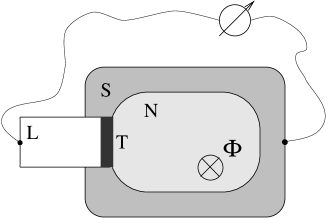
FIG. 1.: Metallic quantum dot (N) in contact with a superconductor (S). A tunnel barrier (T) separates the dot from a normal-metal lead (L) attached for the purpose of making current and voltage measurements.

The system we have in mind is depicted in Fig. 1: a metallic (normal-conducting) quantum dot (N) with the shape of, say, a stadium billiard, is surrounded by a superconductor (S) and contacted by a normal-metal lead (L) via a tunnel barrier (T). A Schottky (or potential) barrier forms at the NS-interface. The quantum dot is pierced by a weak magnetic flux of the order of one or several flux quanta. The temperature is so low that the phase-coherence length exceeds the system size by far. It will help our argument if the quantum dot is not perfectly shaped but contains some defects and/or impurities.

FIG. 2.: (Almost) periodic orbit involving several normal reflections (N) and one Andreev reflection (A). An electron runs through the closed loop twice. Before reaching A it is a particle and afterwards a hole.

The unique feature that distinguishes our quantum dot from conventional mesoscopic systems is the process of Andreev reflection[5], by which an electron incident on the NS-interface is retroreflected as a hole, and vice versa. The drastic consequences of this process for the thermodynamics and the transport of the quantum dot can be anticipated from a semiclassical argument. Consider the periodic orbit of Fig. 2: an electron starts out from point A, undergoes several normal reflections off the Schottky barrier and eventually returns to A, with the final velocity being roughly the negative of the initial one. At the point of return, the electron gets converted into a hole by Andreev reflection. Because the magnetic field is too weak to cause any significant bending of classical trajectories, the hole then simply tracks down the path laid out by the electron. The charge of the hole is opposite to that of the electron, so the magnetic phase accumulated along the total path is zero. Moreover, since a hole is not just the charge conjugate but also the time reverse of an electron, the dynamical phases cancel, too, provided that electron and hole are at the same energy (the Fermi energy). The two Andreev reflections add up to a total phase shift of $\pi$. Thus, the periodic orbit of Fig. 2 contributes to the periodic-orbit sum for the density of states with the negative sign. Orbits of this type reduce the mean density of states (“Weyl term”) and are expected to put our “Andreev quantum dot” in a universality class distinct from the standard Wigner-Dyson ones. We shall identify this universality class in the sequel.

In a microscopic mean-field treatment, we would start from the Bogoliubov-deGennes (BdG) Hamiltonian

$\displaystyle{\cal H}=\pmatrix{H_{0}&\Delta\cr\Delta^{*}&-H_{0}^{*}\cr}$

where $H_{0}=({\bf p}-e{\bf A})^{2}/2m+V({\bf x})-\mu$ is a Hamiltonian for “particles”, $-H_{0}^{*}$ is the corresponding Hamiltonian for “holes”, and the pairing field $\Delta({\bf x})$, whose magnitude rises from zero inside the quantum dot to a nonzero value in the superconductor, converts particles into holes. The potential $V({\bf x})$ includes the Schottky barrier. Energy is measured relative to the chemical potential $\mu$.

Universality classes are characterized by their symmetries. Notice therefore that ${\cal H}$ obeys the relation

$${\cal H}=-{\cal C}{\cal H}^{\rm T}{\cal C}^{-1},\quad{\cal C}=\pmatrix{0&{\bf 1}\cr-{\bf 1}&0\cr}.$$ (1)

This symmetry originates from the electron’s being a spin-1/2 fermion and from spin-rotation invariance [6]. The transformation ${\cal H}\mapsto{\cal C}{\cal H}^{\rm T}{\cal C}^{-1}$ will be called ${\cal CT}$-conjugation as it combines time reversal (${\cal H}\mapsto{\cal H}^{*}={\cal H}^{\rm T}$) with a kind of charge conjugation (${\cal H}\mapsto{\cal CHC}^{-1}$).

By design, the classical motion of particles and holes in the billiard-shaped dot is chaotic and fills the available phase space ergodically. Now observe that every time a particle or hole is Andreev-reflected from the NS-interface, its wavefunction acquires an extra phase determined by the superconducting order parameter. In this context it is important that the applied magnetic field is screened by a supercurrent circulating along the NS-interface inside the superconductor. The supercurrent flow, in turn, is concomitant with a spatial variation of the phase $\phi$ of the order parameter[7]. As a result of this and the chaotic dynamics, the extra phase picked up during Andreev reflection varies randomly along a typical semiclassical trajectory. So everything is quite random, and we expect some kind of random-matrix theory to apply. The question is now: what random-matrix theory?

Because the presence of the magnetic field makes the pairing field experienced by particles and holes vanish on average, $\Delta$ can be modelled by a stochastic variable with zero mean. Moreover, since the system has been designed to be chaotic, there exist no integrals of motion except for energy. The only symmetry (apart from hermiticity of the Hamiltonian) of relevance for the long-time[8] or ergodic limit we shall consider, is the ${\cal CT}$-oddness (1). Experience with similar problems then tells us that we can model the ergodic limit by a Gaussian, or maximum-entropy, ensemble with probability density $\exp(-{\rm Tr}{\cal H}^{2}/2v^{2})d{\cal H}$ subject to the constraint (1). This implies that, in any orthonormal basis of states $\psi_{a}$ $(a=1,{\bar{1}},...,N,{\bar{N}})$ with ${\cal CT}$-conjugate basis $\psi_{\bar{a}}={\cal C}\psi_{a}^{*}$, the variances of the random Hamiltonian matrix elements are given by the correlation law

$$\langle{\cal H}_{ab}{\cal H}_{cd}\rangle=v^{2}(\delta_{ad}\delta_{bc}-\delta_{a\bar{c}}\delta_{b\bar{d}}).$$ (2)

To complete the definition of our random-matrix model, we add to ${\cal H}$ a term $-i\Gamma$ which accounts for the coupling to the normal-metal lead and will be specified later.

As a first step, let us close off the contact with the lead $(\Gamma=0)$. What can we say about the spectral statistics, the central characteristic of the ergodic isolated quantum dot? If $\psi_{k}$ is an eigenstate of ${\cal H}$ with eigenvalue $+E_{k}$ then, by (1), so is ${\cal C}\psi_{k}^{*}$ with eigenvalue $-E_{k}$. Thus, there is an exact pairing between positive and negative eigenvalues. By diagonalizing ${\cal H}$ and computing the Jacobian of the transformation to diagonal form, we obtain the (unnormalized) joint probability density of the positive eigenvalues $E_{k}$ $(k=1,...,N)$:

$$P(E_{1},...,E_{N})=\prod_{i<j}(E_{i}^{2}-E_{j}^{2})^{2}\prod_{k=1}^{N}E_{k}^{2}\ e^{-E_{k}^{2}/2v^{2}},$$ (3)

which is manifestly invariant under $E_{k}\to-E_{k}$[9].

To calculate the spectral statistics, it is convenient to view (3) as a Gaussian Unitary Ensemble (GUE) of $2N$ levels $E_{1},E_{\bar{1}},...,E_{N},E_{\bar{N}}$ with the mirror constraint $E_{\bar{k}}=-E_{k}$. The correlation functions of the GUE are known to coincide with those of a one-dimensional gas of free fermions in the large-$N$ limit[10]. Now, when a fermion (i.e. an energy level) gets close to $E=0$, so does its mirror image. Because Fermi statistics makes the wavefunction vanish as two fermions approach, the constraint $E_{\bar{k}}=-E_{k}$ amounts to hard wall boundary conditions at $E=0$. Hence, we can compute the eigenvalue density and its correlations for (3) as the particle density and its correlations for a free Fermi gas with a hard wall at the origin. In this way we obtain

$$\rho(E)=\langle{\rm Tr}\delta(E-{\cal H})\rangle=1/\delta-\sin(2\pi E/\delta)/2\pi E,$$ (4)

where $\delta$ is the level spacing for $E\gg\delta$. We see that the coupling to the superconductor depletes the mean density of states and makes it vanish quadratically at $E=0$[11]. The states pushed away from $E=0$ cause density oscillations, which ebb off as $1/E$. Note that the result (4) applies when both $E$ and $\delta$ are much smaller than the characteristic energy uncertainty set by the frequency of Andreev reflection.

To understand better the mechanism of depletion, we turn to diagrammatic perturbation theory. Let $G:=\langle(E+i\varepsilon-{\cal H})^{-1}\rangle$ denote the ensemble average of the Gorkov Green’s function. We expand it in a geometric series with respect to ${\cal H}$ as usual. To do the ensemble average, we distinguish between two types of contraction, $\Pi_{ac,bd}^{\rm D}=v^{2}\delta_{ad}\delta_{bc}$ and $\Pi_{ac,bd}^{\rm C}=-v^{2}\delta_{a\bar{c}}\delta_{b\bar{d}}$, corresponding to the first and second term in the basic law (2). Making this distinction is useful for organizing the perturbation series, since $\Pi^{\rm D}$ causes pure GUE behavior whereas $\Pi^{\rm C}$ generates the corrections to the GUE. By summing all nested $\Pi^{\rm D}$ self-energy graphs, we get Pastur’s equation, $G=(E+i\varepsilon-v^{2}{\rm Tr}G)^{-1}$, which is exact for $E\gg\delta$ and $N\to\infty$. The solution, $G^{0}$, of this equation yields Wigner’s semicircle law for the density of states: $-{\rm ImTr}G^{0}/\pi=\sqrt{2N-(E/v)^{2}}/\pi v$. According to (4), corrections to this result, which is stationary and equal to $\sqrt{2N}/\pi v=:1/\delta$ up to uninteresting terms of order $1/N$, should appear as we approach zero energy. It turns out that these arise from summing a geometric series of ladder graphs built solely from $\Pi^{\rm C}$-contractions. The ladder sum, $C_{ac,bd}$, satisfies Dyson’s equation $C=C^{0}+C^{0}\Pi^{\rm C}C$ with $C_{ac,bd}^{0}=\delta_{ab}\delta_{cd}G_{aa}^{0}G_{cc}^{0}$. Its solution $C=C^{0}({\bf 1}-\Pi^{\rm C}C^{0})^{-1}$ is singular at $E=0$:

$\displaystyle C=C^{0}+C^{0}\left(\Pi^{\rm C}2iN\delta/\pi E\right)C^{0}+{\cal O}(E/N)^{0}.$

By evaluating the graph shown in Fig. 3 we get ${\rm Tr}G/\pi=-i/\delta-1/2\pi E+...$, which are the leading terms in a $1/E$ expansion. (There is a renormalization by a factor of 1/2 coming from the possibility of connecting the external legs in Fig. 3 by a nonsingular $\Pi^{\rm D}$ ladder.) This perturbative result is to be compared with the exact formula ${\rm Tr}G/\pi=-i/\delta-[1-\exp(2\pi iE/\delta)]/2\pi E$ reconstructed from (4) by causality. We see that diagrammatic perturbation theory properly reproduces the smooth part of the $1/E$ correction. (The oscillatory term is nonanalytic in the expansion parameter $1/E$ and cannot be recovered by the perturbative summation of graphs.)

What is the semiclassical meaning of the mode $C$? Our diagrammatic analysis suggests an interpretation as a mode of phase-coherent propagation of a particle-hole pair. To gain further insight, recall the periodic orbit shown in Fig. 2. In diagrammatic language, this orbit corresponds to connecting the Green’s function lines in Fig. 3 by just a single $\Pi^{\rm C}$-contraction, and thus is the simplest semiclassical building block of the $C$-mode. More generally, an arbitrary number of Andreev reflections may be inserted into the loop. The only condition is that the particle-hole character of the states during the first and second traversal of the loop be ${\cal CT}$-conjugate to each other. Because ${\cal CT}$-conjugate states carry opposite charge and the loop is traversed twice in the same direction, the $C$-mode is ignorant of a weak magnetic field[12]. Note, however, that the $C$-mode is sensitive to energy $E$ (or voltage), which breaks the phase relation between particles and holes.

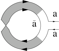
FIG. 3.: Diagram contributing to the average Green’s function in order $1/E$. The shaded region symbolizes the $C$-mode.

With a solid understanding of the spectral properties in hand, we finally open up the tunnel barrier and turn to the prime experimental observable, the conductance $g$. Our treatment will be based on the linear response formula $g=4(e^{2}/h){\rm Tr}{S^{\dagger}}_{\rm ph}S_{\rm hp}$[13] where $S_{\rm hp}$ is the part of the scattering matrix $S$ that maps incoming electrons onto outgoing holes. We suppress elastic phase shifts and parameterize the $S$-matrix by $S={\bf 1}-2i{\tilde{W}}(i\varepsilon+i\Gamma-{\cal H})^{-1}W$ [14] at $E=0$. Here $W$ is a matrix coupling $2M$ channels (particles and holes) in the lead with $2N$ levels in the quantum dot, $\tilde{W}$ is its adjoint, and $\Gamma=W{\tilde{W}}$. $W$ is diagonal in particle-hole space. For a simple model, we take ${\tilde{W}}W$ to be a multiple of the identity in channel space: ${\tilde{W}}W=\gamma{\bf 1}$. Then $\Gamma=\gamma P$ where $P$ is a rank-$2M$ projector in level space. We assume $N\gg M$.

We begin by discussing the limit of an open quantum dot $(M\gg 1)$ where all structure in the density of states is washed out by the large level width. Let $T$ denote the probability for an electron in an incoming channel to be transmitted through the tunnel barrier, in this very limit. For our simple model, $T=4\lambda\gamma/(\lambda+\gamma)^{2}$ with $\lambda^{2}=2Nv^{2}$ [14]. Having entered the quantum dot, the electron spends a long time there, undergoing many Andreev reflections, and finally returns to the lead either as a particle or as a hole, with equal probabilities. Hence $\langle{\rm Tr}{S^{\dagger}}_{\rm ph}S_{\rm hp}\rangle=MT/2$, which we refer to as the “classical” value. To confirm this result diagrammatically, one has to sum a geometric series of $\Pi^{\rm D}$ ladder graphs, producing the diffuson[15]. On approaching the opposite (closed) limit, we expect a reduction relative to the classical value. The reason is simply this: the density of states in the isolated dot vanishes at $E=0$, so that an electron trying to enter cannot find any state to go to and is immediately rejected into the lead. This effect should announce itself as a negative ${\cal O}(M^{0})$ correction (“weak localization”). Such a correction in fact exists and is due to the graph shown in Fig. 4 featuring two diffusons and one $C$–mode. Evaluation of this graph leads to

$$\langle g\rangle=(MT-1+T)\times 2e^{2}/h+{\cal O}(1/MT).$$ (5)

Note that the weak localization correction in the corresponding N-system vanishes. A result similar to (5) was recently found in a related context[16].

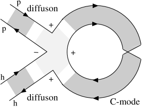
FIG. 4.: Diagram contributing to the average conductance in order $M^{0}$. The shading of the vertex center indicates unitarity-conserving (Hikami box) corrections.

Although the calculation of the graph of Fig. 4 is somewhat technical, the result can easily be checked and interpreted. Consider first the limit of many weakly coupled channels ($T\to 0$, $MT$ fixed). In this limit the absolute square of the Green’s function becomes independent of the level and particle-hole indices, on average[17]. By conservation of probability, the conductance is then fully determined by a one-point function: $\langle g\rangle=-(4e^{2}/h)\bar{\gamma}{\rm Im}\langle{\rm Tr}(i\bar{\gamma}-{\cal H})^{-1}\rangle$ where $\bar{\gamma}=\gamma M/N$ is the mean level width. Analytic continuation of our result for the average Green’s function to $E=i\bar{\gamma}$ gives $\langle g\rangle=(MT-1+e^{-MT})\times 2e^{2}/h$, in agreement with (5).

To understand the other limit of strongly coupled channels $(T=1)$ it is easiest to argue directly at the $S$–matrix level. By its definition as a “sticking probability”, $T=1-|\langle S_{cc}\rangle|^{2}+{\cal O}(1/MT)$. Putting $T=1$ therefore amounts to assuming a fully random $S$-matrix that vanishes on average: $\langle S\rangle=0$. The symmetries of $S$ are the same as those of $\exp i{\cal H}$, so that from (1) we deduce $S={\cal C}{S^{-1}}^{\rm T}{\cal C}^{-1}$, which is the defining equation of the symplectic group ${\rm Sp}(2M,{\bf C})$. (${\cal C}$ is now meant to operate in channel space.) Unitarity fixes a subgroup ${\rm Sp}(2M)$. We are thus led to postulate an $S$-matrix ensemble with probability distribution $\langle\langle\bullet\rangle\rangle$ given by the Haar (or invariant) measure of ${\rm Sp}(2M)$. This ensemble is Dyson’s Circular Unitary Ensemble[1] adapted to fit our particle-hole symmetric situation. By elementary group theory, $\langle\langle S_{ab}\rangle\rangle=0$ and $\langle\langle S_{ab}^{\vphantom{*}}S_{cd}^{*}\rangle\rangle=\delta_{ac}\delta_{bd}/2M$, so $\langle\langle g\rangle\rangle=2Me^{2}/h$, with no correction of order $M^{0}$.

In conclusion, we mention that the singular modes, the diffuson and the $C$-mode, translate into low-energy degrees of freedom of a corresponding nonlinear $\sigma$ model. They determine the attractive (metallic, or free) renormalization group fixed point of this field theory. Ultimately, the existence of such singular modes, which are forgetful of microscopic detail and saturate the long-time and long-distance physics, is the reason why we predict with confidence that the ergodic limit of the chaotic Andreev quantum dot is universal and our random-matrix theory applies.

REFERENCES

- [1] M.L. Mehta, Random Matrices, Academic Press 1991.
- [2] K.B. Efetov, Adv. Phys. 32, 53 (1983).
- [3] R. Gade, Nucl. Phys. B398, 499 (1993); A.V. Andreev, B.D. Simons and N. Taniguchi, Nucl. Phys. B432, 487 (1994).
- [4] R. Oppermann, Physica A167, 301 (1990).
- [5] A.F. Andreev, Zh. Eksp. Teor. Fiz. 46, 1823 (1964).
- [6] Spin-orbit scattering violates the symmetry (1) and drives the system into a separate universality class.
- [7] Note that the choice of gauge is unnatural here as it forces across the lead to be very large.
- [8] Here “long” means times greater than the mean time spent between successive Andreev reflections. In order for the ergodic limit to be nonempty, we require where is defined in the text below Eq. (4).
- [9] Incidentally, the substitution turns this probability density into a member of the family of Laguerre ensembles studied recently by T. Nagao and K. Slevin, J. Math. Phys. 34, 2075 (1993).
- [10] B. Sutherland, J. Math. Phys. 12, 246 (1971); see also B.D. Simons, P.A. Lee and B.L. Altshuler, Phys. Rev. Lett. 72, 64 (1994).
- [11] For lack of space the correlations are not recorded here.
- [12] By this feature, the -mode can be identified as a close relative of the usual (normal-metal) diffuson. It here appears as a separate mode because of our use of the BdG-formalism.
- [13] Y. Takane and H. Ebisawa, J. Phys. Soc. Japan 61, 1685 (1992).
- [14] S. Iida, H.A. Weidenmüller and J.A. Zuk, Ann. Phys. 200, 219 (1990).
- [15] The diffuson is identical to the normal-metal diffuson except that in our case the opposite segments of the ladder are either two BdG-particles or two BdG-holes.
- [16] P.W. Brouwer and C.W.J. Beenakker, Phys. Rev. B52, 3868 (1995).
- [17] M.R. Zirnbauer, Nucl. Phys. A560, 95 (1993).