Folding Transitions of Self-Avoiding Membranes

Abstract

Abstract: The phase structure of self-avoiding polymerized membranes is studied by extensive Hybrid Monte Carlo  simulations. Several folding transitions from the flat to a collapsed state are found. Using a suitable order parameter and finite size scaling theory, these transitions are shown to be of first order. The phase diagram in the temperature-field plane is given.

Fluctuating membranes and surfaces are basic structural elements of biological systems and complex fluids. Recent theoretical work [2, 3] and experimental studies [4, 5] indicate, that these sheetlike macromolecules should have dramatically different properties than linear polymers. Polymerized membranes which contain a permanently cross-linked network of constituent molecules have a shear elasticity, giving them a large entropic bending rigidity. In the absence of self-avoidance, polymerized [6] and fluid [7] membranes adopt a crumpled random structure. Theoretical predictions by Flory mean-field approximation and Monte Carlo simulations [6] and renormalization group studies [8] supported the existence of a high temperature crumpled phase for self-avoiding polymerized membranes also, suggesting a possible finite temperature crumpling transition in the presence of an explicit bending rigidity [9]. However, more extensive computer simulations [3, 10, 11, 12] found no crumpling of self-avoiding tethered membranes in a good solvent. This prediction was confirmed recently by experimental studies of graphitic oxide [4].

On the other hand, polymerized vesicles undergo a wrinkling transition [5], and upon addition of 10 vol % acetone, Spector and co-workers [4] found small compact objects, which appeared to be folded. A poor solvent leads to (short-ranged) attractive interactions, and a single membrane was found to be flat for high temperatures [10], but in a collapsed state for sufficiently low temperatures [3]. The transition between the flat and the collapsed states of the membrane proceeds through a sequence of folding transitions, which were first found by cooling of a single membrane from the flat phase [13]. Because no hysteresis was found, it was ruled out that the folded configurations are metastable states. However, this method does not give sufficient evidence of the order or even the existence of a transition. For instance, hysteresis can also be found at second order phase transitions of finite systems and the results for one system size may be misleading. In addition, the experimentally observed wrinkling transition is first order [5].

On that account, we present a systematic finite size scaling analysis of the folding transitions. The Hybrid Monte Carlo  algorithm was used, which provides for simulations of the canonical ensemble with constant temperature. Moreover, ensemble averages are independent of the discretization step size ${\delta}t$, i.e. systematic errors [14, 15]. A suitable order parameter is defined and a phase diagram is presented.

Besides the nearest neighbour interactions, the membranes were modeled similar to those of Abraham and Kardar [13]. The $N$ particles of the polymerized membrane form the sites of a hexagonal shaped triangular lattice. The bond potential between nearest neighbour particles is

$$V^{\mbox{{B}}}=\sum_{j(i)}{\left({b_{0}-r_{ij}}\right)}^{2}\quad,$$ (1)

with an equilibrium length $b_{0}$ and distances $r_{ij}$ between particle $i$ and its nearest neighbors $j(i)$. In place of this harmonic potential, tethers were used by Abraham and Kardar [13].

All particles interact through a shifted Lennard-Jones potential

$$V^{\mbox{{LJ}}}_{ij}=\left\{\begin{array}[]{ccc}\left({\frac{1}{r_{ij}^{12}}-2\frac{1}{r_{ij}^{6}}}\right)+\left({\frac{1}{r_{c}^{12}}-2\frac{1}{r_{c}^{6}}}\right)&,&r_{ij}<=r_{c}\\ 0&,&r_{c}<r_{ij}\end{array}\right.$$ (2)

with a cut-off at $r_{c}~{}=~{}2.5$  . The repulsive part of this interaction guarantees self-avoidance of the membrane.

The folding of the membrane can be described by the eigenvalues ${\lambda_{1}}^{2}~{}>=~{}{\lambda_{2}}^{2}~{}>=~{}{\lambda_{3}}^{2}$ of the inertia tensor

$${\cal T}_{\alpha,\beta}=\frac{1}{N}\sum_{i=1}^{N}\left({r_{i\alpha}r_{i\beta}-\overline{r}_{\alpha}\overline{r}_{\beta}}\right)\quad,$$ (3)

where $\alpha,\beta\in\{x,y,z\}$, and the sum runs over all particles of a given configuration; $\overline{r}_{\alpha}$ is the $\alpha$ component of the center of mass for a configuration. We can estimate the expected change of the membrane eigenvalues by those of an unfolded or folded disc with radius $1$ and width $d=0.1$ as shown in Table I. Taking into account all three eigenvalues, an unfolded, folded or twice folded configuration can be distinguished. A collapsed configuration would be indicated by approximately equal eigenvalues.

Membranes with up to $N=1141$ particles were simulated at inverse temperatures in the range $\beta\in[0.2;0.75]$. Configurations at $\beta=0.20$, $0.27$ and $0.40$ were found to be in an unfolded, folded and twice folded state by visualization (figure not shown).

At the first folding transition, the eigenvalue $\lambda_{1}^{2}$ stays constant approximately, while the second eigenvalue $\lambda_{2}^{2}$ decreases by a factor $c~{}{\approx}~{}0.2790$. Therefore, we define an order parameter $m$ by

$$\langle{m(\beta)}\rangle=\left\langle{\frac{1}{\left({1-\sqrt{c}}\right)}\left[{\frac{\lambda_{2}(\beta)}{\lambda_{2}(\beta_{0})}-\sqrt{c}}\right]}\right\rangle\quad,$$ (4)

where ${\lambda_{2}(\beta_{0})}$ is a reference value of an unfolded membrane at $\beta_{0}$ far below the inverse critical temperature $\beta_{c}$. At a first order transition, the average order-parameter discontinuously jumps at $\beta_{c}$ [16, 17, 18]. Contrary, at a continuous phase transition we expect a power law behavior of the average order parameter $\langle{m}\rangle(\beta)$ with an exponent $\beta^{\prime}$, i.e. $\langle{m}\rangle\propto{\left({\beta-\beta_{c}}\right)}^{\beta^{\prime}},\beta>\beta_{c}$ [19, 20, 21, 22]. Indeed, the average order parameter $\langle{m}\rangle$ becomes very steep near $\beta_{c}$ with increasing number of particles $N$ (data not shown). In principle, one can measure the increase of the slope and compare to the predictions of finite size scaling theory. Of course, the slope of $\langle{m}\rangle(\beta)$ is proportional to the susceptibility $\chi$, which can be measured by the fluctuations of $m$ also:

$$\chi(\beta)=L^{d}\beta\left({{\langle{m^{2}}\rangle}_{L}-{\langle{m}\rangle}_{L}^{2}}\right)$$ (5)

The susceptibility $\chi(\beta)$ is shown in Figure 1 and the scaling of the maximum $\max{\chi(\beta)}$ in the inset of Figure 1.

At a first order transition, $\chi(\beta_{c}^{\mbox{eff}})$ is expected to increase proportional to $N=L^{d}$ [16, 17, 18]. At a continuous phase transition, ${\left|{\beta-\beta_{c}}\right|}^{-\gamma_{\pm}}$ is predicted [19, 20, 21, 22]. The $L^{d}$ increase of $\chi(\beta)$ in Figure 1 gives evidence of the scaling at a first order transition. In addition, the width of the susceptibility peak should decrease as $L^{-d}$ [16, 17, 18]. Figure 2 shows a finite size scaling plot of the susceptibility data. Within errors, first order scaling behavior can be observed, at least above the inverse transition temperature.

The transition temperature $\beta_{c}^{\infty}$ can be extrapolated by the position of the maximum in $\chi(\beta)$ [18], the minimum of the cumulant [18] and the equal weight criterion [24] of the order parameter distribution. At least for $\chi$, the equal weight criterion predicts a shift of the effective transition temperature proportional to $L^{-2d}$ [23, 24, 25], whereas a shift proportional to $\propto L^{-1/\nu}$ is expected for a continuous phase transition. Using quadratic terms in the regression, the extrapolations in Figure 3 of the three observables agree within errors. The transition temperature of the first folding transition is found to be $\beta_{c}^{\infty}=0.247(5)$.

The increase of the susceptibility is caused by the characteristic double-peak structure of the order parameter distribution near $\beta_{c}$, which is typical for a discontinuous phase transition [16, 17, 18, 19, 23, 24, 25, 26]. Figure 4 shows the expected double-peak distribution $P(m)$ at the equal height transition temperature [24]. The development of a minimum in $P(m)$ is confirmed by the method of Lee and Kosterlitz [26]. The measured ${\Delta}F$ in the inset of Figure 4 is proportional to the free energy difference at the equal height transition temperature and increases as ${(L^{d})}^{x}$, $x{\approx}1.3$.

Further, $P(m)$ can be described by the reduced cumulant $U_{L}$

$$U_{L}(\beta)=1-\frac{{\langle{m^{4}}\rangle}_{L}}{3{\langle{m^{2}}\rangle}^{2}_{L}}\quad.$$ (6)

At a continuous phase transition, $U_{L}(\beta)$ is expected to approach $2/3$ for all $\beta$. The data shows a minimum, which becomes more pronounced for large $N$, indicating a first order phase transition (figure not shown).

The folding of the membrane must be visible in the attractive part of the potential energy, also. In fact, there is a jump in the potential energy and the related specific heat develops a peak, although very slowly. Besides the above defined order parameter, which is based on the geometry of the membrane, we can derive a different order parameter from the attractive part of the Lennard-Jones potential:

$$\tilde{m}=\frac{1}{N}\left\{\sum_{i<j}\Theta\left({r_{c}-r_{ij}}\right)\left({2\frac{1}{r_{ij}^{6}}+2\frac{1}{r_{c}^{6}}}\right)\right\}\quad.$$ (7)

Compared to $m$, the order parameter $\tilde{m}$ has the advantage, that it is a local property. We performed Hybrid Monte Carlo  simulations with an additional term $h{\cdot}\tilde{m}$ in the Hamiltonian, where $h$ is the conjugate field. Figure 5 shows the phase diagram in the $(\beta,h)$-plane of a membrane with $271$ particles. The first order transition lines were computed by the multi-histogram method [27]. For the transition from one to two folds, an order parameter similar to $m$ is used, which is based on $\lambda_{1}$ instead of $\lambda_{2}$. $h=1$ is an upper limit for both transition lines, because of the vanishing attractive interactions at $h=1$.

The main result of this study is the first order nature of the folding transitions of self-avoiding polymerized membranes. This is in agreement with the observed folded structure of graphitic oxide [4] and the first order wrinkling transition of partially polymerized vesicles [5].

Recently, another first order folding transition was found by DiFrancesco and Guitter [28] for regular triangular lattices embedded into two-dimensional space. However, these transitions combine flat and compact states directly, i.e. without several distinct foldings. Therefore, the folding transition described here is of a different kind.

The unfolding of a singly folded membrane bears close resemblance to the unbinding transition of two distinct surfaces. Regarding a folded membrane of $N$ particles, the fraction of particles near the crease decreases with $1/\sqrt{N}$. Therefore, the nature of the folding transition is related to the nature of the underlying unbinding transition of two distinct membranes without the crease. The shape fluctuations of a single membrane of lateral size $\xi_{\parallel}$ are characterized by the typical fluctuation amplitude $\xi_{\perp}\propto{\xi_{\parallel}}^{\zeta}$. Polymerized membranes without lateral tension have a roughness exponent $\zeta\approx 0.6$. The steric hindrance of two interacting membranes at separation $l$ leads to an overall loss of entropy, which can be regarded as an effective fluctuation-induced repulsion, $V_{rep}\propto{1/{l^{\tau}}}$ with decay exponent $\tau\approx 3.3$ for polymerized membranes. This repulsive interaction causes the unfolding of the membrane even in the presence of attractive van der Waals interactions. However, the crease of the folded membrane introduces an additional attractive interaction. This situation is similar to a membrane interaction which exhibits two minima at two different separations. Such an interaction implies a first-order unbinding transition [29] and may be an explanation of the first-order folding transition described in this work.

Further investigations are necessary to determine the nature of the relation between folding and unbinding of polymerized membranes.

configuration	${\lambda_{1}}^{2}$	${\lambda_{2}}^{2}$	${\lambda_{3}}^{2}$
disc	$0.2543$	$0.2473$	$0.00084$
disc, folded	$0.2524$	$0.0690$	$0.00332$
disc, folded twice	$0.0929$	$0.0487$	$0.01330$
disc	$1.0000$	$1.0000$	$1.00$
disc, folded	$0.9925$	$0.2790$	$3.95$
disc, folded twice	$0.3653$	$0.1969$	$15.83$

TABLE I.: Eigenvalues of the moment of inertia tensor of a disc with radius $1$ and width $d=0.1$. In the lower part, all numbers are relative to the values of the unfolded disc.

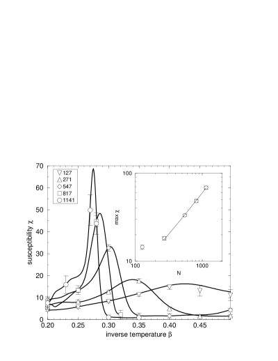
FIG. 1.: Susceptibility ${\chi}(\beta)$ for membranes with $N=127,271,547,817$ and $1141$ particles. The solid lines were computed by the multi-histogram method. The scaling of the maximum $\max{\chi}$ is shown in the inset.

FIG. 2.: Finite size scaling plot of the susceptibility $\chi(\beta)$ for a first order transition using the value $\beta_{c}^{\infty}=0.247(5)$ from Figure 3.

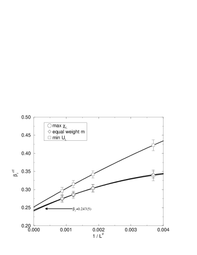
FIG. 3.: Critical temperature $\beta_{c}^{\infty}=0.247(5)$ determined by the position of the maximal susceptibility $\chi$, the minimum of the cumulant $U_{L}$ and equal-weight of the order parameter distribution for the four largest system sizes.

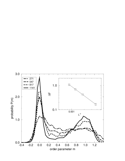
FIG. 4.: Probability distribution $P(m,\beta_{ew})$ of the order parameter $m$ at the equal-weight transition temperature $\beta_{ew}$. The inset shows the free energy difference ${\Delta}F$ at the equal-height transition temperature $\beta_{eh}$, which increases $\propto{(L^{d})}^{x}$, $x{\approx}1.3$.

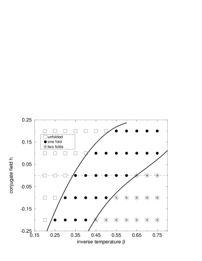
FIG. 5.: Phase diagram of a membrane with $271$ particles in the $\beta,h$ plane. The symbols denote the result of the simulations, the solid lines are the first order transition lines computed by the multi-histogram method.